Numerical Simulations to Predict the Thermal Response of Insulating Concrete Form (ICF) Wall in Cold Climate

Publisher’s version / Version de l'éditeur:

Vous avez des questions? Nous pouvons vous aider. Pour communiquer directement avec un auteur, consultez la première page de la revue dans laquelle son article a été publié afin de trouver ses coordonnées. Si vous n’arrivez pas à les repérer, communiquez avec nous à PublicationsArchive-ArchivesPublications@nrc-cnrc.gc.ca.

Questions? Contact the NRC Publications Archive team at

PublicationsArchive-ArchivesPublications@nrc-cnrc.gc.ca. If you wish to email the authors directly, please see the first page of the publication for their contact information.

https://publications-cnrc.canada.ca/fra/droits

L’accès à ce site Web et l’utilisation de son contenu sont assujettis aux conditions présentées dans le site

LISEZ CES CONDITIONS ATTENTIVEMENT AVANT D’UTILISER CE SITE WEB.

Research Report (National Research Council of Canada. Institute for Research in Construction), 2011-04-01

READ THESE TERMS AND CONDITIONS CAREFULLY BEFORE USING THIS WEBSITE. https://nrc-publications.canada.ca/eng/copyright

NRC Publications Archive Record / Notice des Archives des publications du CNRC :

https://nrc-publications.canada.ca/eng/view/object/?id=034e16bf-dc30-43eb-9ac4-c9a16fe1380b https://publications-cnrc.canada.ca/fra/voir/objet/?id=034e16bf-dc30-43eb-9ac4-c9a16fe1380b

NRC Publications Archive

Archives des publications du CNRC

For the publisher’s version, please access the DOI link below./ Pour consulter la version de l’éditeur, utilisez le lien DOI ci-dessous.

https://doi.org/10.4224/20374494

Access and use of this website and the material on it are subject to the Terms and Conditions set forth at

Numerical Simulations to Predict the Thermal Response of Insulating Concrete Form (ICF) Wall in Cold Climate

Saber, H. H.; Maref, W.; Armstrong, M. M.; Swinton, M. C.; Rousseau, M. Z.; Gnanamurugan, G.

http://www.nrc-cnrc.gc.ca/irc

N um e ric a l Sim ula t ions t o Pre dic t t he T he rm a l Re sponse of I nsula t ing Conc re t e Form (I CF) Wa ll in Cold Clim a t e

I R C - R R - 3 1 0

A p r i l 2 0 1 1

The material in this document is covered by the provisions of the Copyright Act, by Canadian laws, policies, regulations and international agreements. Such provisions serve to identify the information source and, in specific instances, to prohibit reproduction of materials without written permission. For more information visit http://laws.justice.gc.ca/en/showtdm/cs/C-42

Les renseignements dans ce document sont protégés par la Loi sur le droit d'auteur, par les lois, les politiques et les règlements du Canada et des accords internationaux. Ces dispositions permettent d'identifier la source de l'information et, dans certains cas, d'interdire la copie de documents sans permission écrite. Pour obtenir de plus amples renseignements : http://lois.justice.gc.ca/fr/showtdm/cs/C-42

Numerical Simulations to

Predict the Thermal Response

of Insulating Concrete Form

(ICF) Wall in Cold Climate

Research Report RR-310

Date: April 1, 2011

Authors:

Hamed H. Saber, Wahid Maref, Marianne Armstrong, Michael C.

Swinton, Madeleine Z. Rousseau, and Ganapathy

Gnanamurugan

ACKNOWLEDGMENTS

The authors wish to thank Anil Parekh at Natural Resources Canada (NRCan) and Silvio Plescia at Canada Mortgage and Housing Corporation (CMHC) for providing guidance and contributing funding for this project. Funding from NRC has enabled NRC-IRC to build, operate and maintain a state-of-the-art Field Exposure of Walls facility (FWEF). Our thanks are also extended to Ross Monsour at Ready Mix Concrete Association of Ontario (RMCAO) for his contribution in providing the test specimens and NRC-IRC colleague Mike Nicholls for his precious technical contribution.

EXECUTIVE SUMMARY

Field monitoring of the dynamic heat transmission characteristics through Insulating Concrete Form (ICF) wall assemblies was undertaken in 2009-2010 at National Research Council Canada’s Institute for Research in Construction’s (NRC-IRC) Field Exposure of Walls Facility (FEWF). The main objective of this research is to evaluate the dynamic heat transmission characteristics through two mid-scale ICF wall assemblies in FEWF for a one year cycle of exposure to outdoor natural weathering conditions. The scope of work included the design of the experiments, installation of test specimens, commissioning of the instrumentation, operation of the test facility, monitoring, and data collection & analysis. The present NRC-IRC’s hygrothermal model, called hygIRC-C, was used to interpret the readings of the instrumentations and to improve the experiment design by repositioning these instrumentations at critical locations. Subsequently, the present model was benchmarked against the measured data. Results showed that the predictions of the present model are in good agreement with experimental data. This research is on-going. Future work will be presented in later publications where the present model will be used to conduct numerical simulations in order to investigate the transient thermal response of full-scale ICF wall assemblies subjected to different Canadian climates.

TABLE OF CONTENTS ACKNOWLEDGMENTS

………i

EXECUTIVE SUMMARY ………. ii

1  INTRODUCTION and Background ... 1 

2  ICF WALL ASSEMBLIES AND INSTRUMENTATION ... 5 

3  GENERAL PARAMETERS AFFECTING THE THERMAL RESPONSE OF WALL SYSTEMS ... 6 

4  Governing Equations ... 10 

4.1  Initial and Boundary Conditions ... 11 

5  RESULTS AND DISCUSSIONS ... 14 

6  Effect of Thermal Mass ... 25 

7  SUMMARY AND CONCLUSION ... 34 

8  References ... 35 

LIST OF TABLES Table 1. Dimension and thermal properties of the ICF components and glass fibre ... 8 

LIST OF FIGURES Figure 1. Schematic of ICF wall specimens showing the instrumentation (heat flux transducers, HF, and thermocouples, TC) and 3D representation of half of ICF wall .. 6 

Figure 2. Measured thermal conductivity of the EPS ... 7 

Figure 3. Measured temperatures at vinyl siding –exterior EPS and drywall – interior EPS interfaces ... 13 

Figure 4. Predicted temperature contours at end of simulation (time = 161.66 day) ... 15 

Figure 5 Installation of heat flux transducer in the ICF test specimen. ... 16 

Figure 6. Predicted heat flux at different locations in the interior EPS layer at the center of wall ... 19 

Figure 7 Comparison of predicted and measured heat fluxes in the interior EPS layer at the center of wall ... 20 

Figure 8 Predicted heat flux at different locations in the exterior EPS layer at the center of wall ... 21 

Figure 9 Comparison of predicted and measured heat fluxes in the exterior EPS layer at the center of wall ... 22 

Figure 10 Enlargement of Figure 9 during a period of 2 weeks (time = 56d – time = 70 d) 23  Figure 11. Comparison of predicted and measured heat fluxes at vinyl siding – EPS interface at the center of wall ... 24 

Figure 12. Schematic of ICF wall with and without concrete ... 27 

Figure 13. Snapshot of the vertical velocity contours (in mm/s) in the air layer between vinyl siding and external EPS layers at the end of simulation... 28 

Figure 14. Predicted heat flux on the indoor surface of gypsum board in the cases of ICF walls with and without concrete layer ... 29 

Figure 15. Cumulative energy loss for walls with and without concrete layer ... 30 

Figure 16. Yearly cumulative energy loss for walls with and without concrete layer ... 31 

Figure 17. Cumulative energy gain for walls with and without concrete layer ... 32 

1 INTRODUCTION AND BACKGROUND

Increasingly, home builders are turning towards a variety of construction methods to improve thermal performance while reducing the cost of construction. While Insulating Concrete Form (ICF) technology dates back to the late 1960s in Europe, ICF construction has only caught on in North America for use in residential and commercial construction over the last two decades (Hersh Servo AG, 2010). Generally modern ICFs consist of stackable formwork made of expanded polystyrene foam, which is filled on site with concrete, and then remains in place to provide permanent insulation. ICF technology offers the potential to improve air tightness and energy performance over the current practice of wood frame construction. With the growing presence of ICF construction in the market, it is important to gain an understanding of their actual performance in the field, and the role played by the thermal mass of the concrete in regulating heat losses.

A number of research projects have been performed on the thermal performance and thermal mass to investigate the potential of annual energy saving compared to traditional light-weight construction for example. The benefit of thermal mass was extensively investigated, especially at the Oak Ridge National Laboratory (Burch et al., 1984a, Burch et al., 1984b, Burch et al., 1984c, Christian, 1991, Kosny et al., 1998, Kosny et al., 2001, and Kossecka and Kosny, 1998). Petrie et al. (2001) conducted field investigation of two side-by-side houses in Knoxville, Tennessee. The two houses were similar except one house had Insulating Concrete Form (ICF) exterior walls and the other house had conventional wood-framed exterior walls. The results showed that the ICF house used 7.5% less energy than the conventional house. This work has shown that the principal benefit of thermal mass on thermal performance is to dampen fluctuations in interior conditions during significant fluctuations in outdoor conditions. Additionally, Petrie et al. (2001) conducted numerical simulations using DOE2 software to investigate the effect of different climates of six US cities (Phoenix, Minneapolis, Dallas, Boulder, Knoxville and Miami) on the energy consumption of both the ICF and conventional wood-framed houses. The results of cooling, heating and total electricity usage showed that the thermal mass had benefits for both cooling and heating. The ICF houses used 5.5% to 8.5% less energy annually than the conventional wood-framed houses. This range of saving (5.5% to

8.5%) agreed with Kosny’s prediction of 4% to 10% savings with ICF houses compared to conventional wood-framed houses for 10 US climates (Kosny et al., 2001).

In 1999, NAHB Research Centre tested 3 side-by-side homes with floor area of 102 m2 (1098 ft2) to compare the energy performance of two ICF homes (one had an ICF plank system and one had an ICF block system) versus conventional wood-framed home (2x4 wall stud framing, sheathed with OSB, and insulated with fiberglass batt in the wall cavities). The three homes were located on the same street in Chestertown, Maryland. Also, the three homes had identical orientation, window area, roof construction, footprint, ductwork, and air handler systems. The testing was conducted over a one-year period beginning in April 1998. Heating consumption composed of two periods, April 1, 1998 through June 1, 1998 and October 6, 1998 through March 16, 1999. Cooling consumption represented the period from June 1, 1998 through September 22, 1998. This study showed that a 20% difference was noticed between ICF houses and the conventional wood-frame house’s energy consumption. This difference can be attributed primarily to the higher effective R-value of the ICF walls and continuous insulation at the slab. The insulation for the walls of the ICF homes is R-20 while the wall insulation of the wood-framed home is R-13. The solid wall surfaces for all three homes make up approximately 44% of the total surface area of the homes (the remainder being made up of the ceiling area, windows, and doors). A 50% increase in the solid wall surface area resistance to conductive heat loss (R-20 compared to R-13) represented significant increased energy-efficiency. The foundation/slab details showed the impact clearly on the wood-frame home and was demonstrated greater heat loss in February and greater heat gain in August as evidenced by the wood-frame home’s more pronounced and direct response to outdoor temperature changes. Given the total area and the thermal conductivity of materials involved, the foundation/insulation/slab detail of the wood-frame home represented a significant source of heat loss and gain not evidenced in the ICF homes.

In 2001, the Portland Cement Association conducted a modeling study of the energy use of single-family houses with various exterior walls using DOE 2.1 software (Gajda, 2001). This study presented two ICF options: (1) concrete sandwiched by two insulation layers, and (2) insulation sandwiched by two concrete layers. The study examined the performance of eleven

different types of exterior walls in 25 North American locations to determine the expected differences in energy use. In this study, the only differences for a given location were the exterior wall type and the capacity of the HVAC system. The results showed that houses with concrete walls had lower heating and cooling costs than walls with light construction, and contributed to additional savings through a reduction in the required heating and cooling system capacity.

In 2006, a project was conducted by Enermodal Engineering Limited for Canada Mortgage and Housing Corporation (CMHC) and the Ready Mix Concrete Associate of Ontario (RMCAO) to study the performance of a 7-storey insulating concrete form multi-residential building in Waterloo, Canada (Hill and Monsour, 2006). Temperatures through the wall assembly were monitored at eight locations from December 1st, 2005 to February 26th, 2006. The project reported little contribution of the concrete to the steady-state R-value. During transient conditions, heat storage effects were reported. While the concrete never supplied heat to the interior during the winter monitoring period, the measured data showed that concrete did temper heat loss to the exterior during the periods of cold weather.

Recently, the National Research Council of Canada’s Institute for Research in Construction (NRC-IRC) in collaboration with Canada Mortgage and Housing Corporation (CMHC) and Natural Resources Canada (NRCan) proposed evaluating the thermal response of two ICF wall assemblies in NRC-IRC’s Field Exposure of Walls Facility (FEWF) for one year cycle of exposure to outdoor natural weathering conditions. The FEWF allows field monitoring of the thermal response of side-by-side test wall specimens exposed to natural weathering on the exterior and exposed to controlled indoor conditions.

This research report presents information generated from this project in order to understand and quantify the effect of thermal mass of the concrete in the ICF wall systems in Canadian cold climate. In previous publication by the authors, the results of the first period of the test (166.66 days) were presented (see Saber et al., 2010d). The objective of this research report is to use the present NRC-IRC’ hygrothermal model called “hygIRC-C” used to interpret the readings of the instrumentations and to improve the experiment design by selecting the appropriate locations of instrumentation. Next, the present model is benchmarked by comparing its prediction against the

test results. After gaining confidence in the simulation tool, it will be used to investigate the effect of thermal mass of the concrete and EPS on the thermal response of the ICF assembly subjected to Canadian climate conditions.

The hygIRC-C model uses COMSOL Multiphysics (www.comsol.com) as a solver. This model solves simultaneously the highly nonlinear 2D and 3D Heat, Air and Moisture (HAM) equations. These equations were discretized using the Finite Element Method (FEM). This model has been used in several related studies (Elmahdy et al., 2009, Saber et al., 2010a and 2010b, 2010c, 2010d, Saber and Swinton, 2010, Saber et al., 2011a and 2011b, 2011c). The 3D version of this model was used to conduct numerical simulations for different full-scale wall assemblies with and without penetration to represent window in order to predict the effective thermal resistance (R-value) with and without air leakage. These walls incorporated two different types of insulation, specifically, spray polyurethane foam and glass fibre. The predicted R-values for these walls were in good agreement (within ± 5%) with the measured R-values in NRC-IRC’s Guarded Hot Box (GHB) (Elmahdy et al., 2009, and Saber et al., 2010a, 2011a). Recently, the 2D version of the present model was used to conduct numerical simulations in order to investigate the effect of the emissivity of foil on the effective thermal resistance of a foundation wall system with foil bonded to expanded polystyrene foam in a furred assembly with airspace next to the foil (Saber and Swinton, 2010 and Saber et al., 2011b). In this work (Elmahdy et al., 2009, Saber et al., 2010a, 2011a, Saber and Swinton, 2010 and Saber et al., 2011b), no moisture transport was accounted for in predicting the thermal performance of different types of walls.

In the case of accounting for moisture transport, the present model was used to predict the drying rate of a number of wall assemblies subjected to different exterior and interior boundary conditions (Saber et al., 2010b). The results showed that the overall agreements between the present model and the hygIRC-2D model that was previously developed and benchmarked at NRC-IRC (Maref et al., 2002) as well as the experimental measurements were good in terms of the shapes of the drying and drying rate curves. Additionally, the predicted average moisture content of the different wall assemblies over the test periods were in good agreement, all being within ±5% of those measured. Another step for benchmarking the present model is to compare its predictions against field measurements as opposed to controlled lab of the thermal response of

mid-scale ICF walls as will be shown in this report. As indicated earlier, these walls are being tested and subjected to different exterior and interior conditions. The descriptions of the wall specimens and experimental approach are briefly discussed in the next sections.

2 ICF WALL ASSEMBLIES AND INSTRUMENTATION

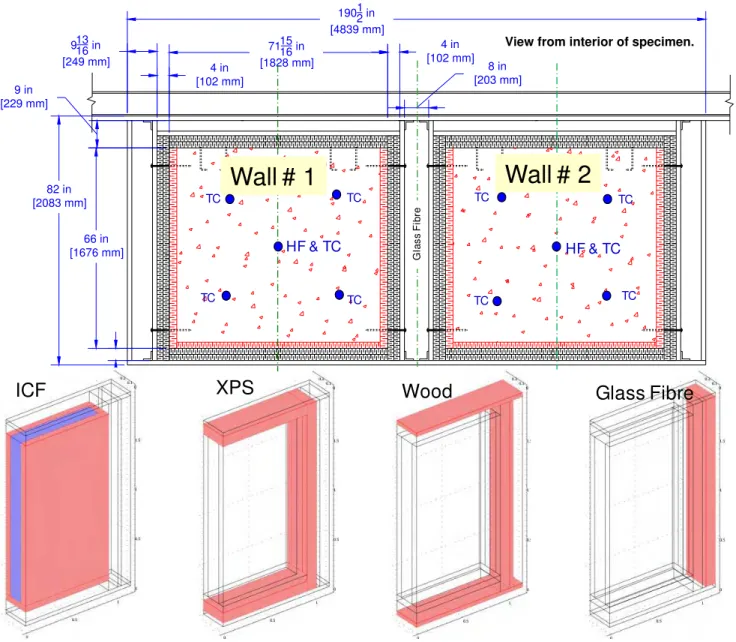
Two ICF wall test specimens were installed side-by-side in the FEWF. The dimensions of the test specimens are shown in Figure 1. For repeatability purposes, the two test specimens were identical in order to provide an indication of the variability of results under similar exposure conditions. Prior to preparing the two ICF specimens, the present model was used to determine the thickness of the thermal insulation needed around and between the ICF specimens to minimize the thermal interaction between the specimens and the rest of the FEWF walls. The ICF wall is comprised of an external layer of expanded polystyrene foam, EPS (nominal thickness of 2.5”), a layer of concrete (6” thick) and an interior layer of EPS (2.5” thick). The ICF has plastic spanners to connect the layers of EPS and reinforced with horizontal and vertical steel bars prior to pouring the concrete. The specimens were allowed to cure outdoors for 28 days before being lifted into place by forklift on August 25th 2009. The ICF test specimens were covered with a painted drywall on the interior. The exterior of the ICFs were covered by a vinyl siding that is resistant to rainwater ingress, as rain water ingress and its effects on heat transmission characteristics are not intended to be included in the study.

In each wall specimen, four heat flux transducers were installed at the center of the wall as shown in Figure 1 at the following interfaces: (1) between the vinyl siding and the exterior EPS foam layer, (2) on the face of the concrete behind the exterior EPS foam layer, (3) on the face of the concrete behind the interior EPS foam layer, and (4) between the drywall and the interior EPS foam layer. At each of these interfaces, two thermocouples were installed at each of the five instrumentation locations shown in Figure 1, for a total of 10 thermocouples per interface. As a part of the test protocol, all heat flux transducers used in the two ICF test specimens were calibrated according to the ASTM C 1130-07 “Standard Practice for Calibrating Thin Heat Flux Transducers”. The uncertainly of heat flux measurements was ± 5%. Also, the uncertainty of thermocouples measurements was ± 0.1oC. More details about the test protocol and results will

be presented in later publications.

View from interior of specimen. 190₂1 in [4839 mm] 82 in [2083 mm] 4 in [102 mm] 4 in [102 mm] 8 in [203 mm] 7115₁₆ in [1828 mm] 66 in [1676 mm] 9 in [229 mm] 913₁₆ in [249 mm] 4 in [102 mm]

ICF XPS _{Wood Glass Fibre}

Wall # 1

Wall # 2

Figure 1. Schematic of ICF wall specimens showing the instrumentation (heat flux transducers, HF, and thermocouples, TC) and 3D representation of half of ICF wall

3 GENERAL PARAMETERS AFFECTING THE THERMAL

RESPONSE OF WALL SYSTEMS

and Monsour, 2006). Recently, the thermal conductivity and density of the type of EPS layer that was used in the ICF wall were measured at the NRC-IRC’s material characterization laboratory at different temperatures. The test method used to measure the thermal conductivity of EPS was ASTM C 518-04 (2007). The measured thermal conductivity of EPS, λeff (in

W/(mK)), as a function of temperature, T (in oC), that was used in the numerical simulation is given as:

Figure 2. Measured thermal conductivity of the EPS

0.029 0.030 0.031 0.032 0.033 0.034 -10 -5 0 5 10 15 20 25 30 λ eff

= 1.062E-4*T+0.0308

+1.5%

-1.5%

Temperature, T (

C)

Th

ermal Co

nduct

iv

it

y,

λ

(W

/(mK))

0308 . 0 10 062 . 1 × 4 + = − T eff λ (1)

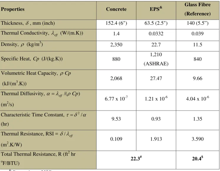
The measured thermal conductivity of the EPS as a function of temperature is shown in Figure 2. As shown in this figure, the uncertainty of the measured thermal conductivity of EPS was ±1.5%. The measured density of EPS was 22.7 kg/m3 (uncertainty = ±0.6 kg/m3). Also, the thermal properties of glass fibre with a thickness of 140 mm that can fill the stud cavities of a 2”x6” wood frame construction are listed in Table 1 as a reference just for a purpose of explaining the effect of material properties on the transient response of wall systems.

Table 1. Dimension and thermal properties of the ICF components and glass fibre

Properties Concrete EPS& Glass Fibre

(Reference)

Thickness, δ , mm (inch) 152.4 (6") 63.5 (2.5") 140 (5.5”)

Thermal Conductivity, λ_eff (W/(m.K)) 1.4 0.0332 0.039

Density, ρ (kg/m3) 2,350 22.7 11.5

Specific Heat, Cp (J/(kg.K)) 880 1,210

(ASHRAE) 840

Volumetric Heat Capacity, ρCp

(kJ/(m3 .K))

2,068 27.47 9.66 Thermal Diffusivity, α =λ_eff /( Cpρ )

(m2/s)

6.77 x 10-7 1.21 x 10-6 4.04 x 10-6 Characteristic Time Constant, τ =δ2/α

(hr) 9.53 0.93 1.35

Thermal Resistance, RSI = δ/λ_eff (m2.K/W)

0.109 1.913 3.590 Total Thermal Resistance, R (ft2 hr

o F/BTU) 22.3 # 20.4$ & Properties at 23oC $

value does not include the effect of thermal bridging due to 2” x 6” studs #

There are four main parameters that affect the thermal response of a wall system. These parameters are:

1. Volumetric heat capacity, sometimes called thermal mass. This is a measure of the ability of the material to store thermal energy. In the case of the ICF wall, the concrete has the ability to store energy of 75 times that for EPS. Furthermore, the ICF wall has the ability to store thermal energy of ~ 200 times that for glass fibre. 2. Thermal diffusivity, α =λ_eff /( Cpρ )_{. This is the ability of the material to conduct}

thermal energy relative to its ability to store thermal energy. The material with low thermal diffusivity responds slower to changes in the thermal environment compared to that with high thermal diffusivity. As shown in Table 1, the EPS and glass fibre respond to the thermal changes 3 times and 6 times, respectively, faster than the concrete.

3. Thermal resistance (R-value). It is a measure of the material ability to resist the heat flow. As shown in Table 1, both the ICF components and the glass fibre in reference wall have approximately the same R-value of (R-20). Unlike the ICF wall, the reference wall with glass fibre has thermal bridges through the wood/steel studs. In a recent study at NRC-IRC (Elmahdy et al., 2009 and Saber et al., 2010a), the measured R-value in the NRC-IRC’ Guarded Hot Box (GHB) for a full-scale glass fibre wall assembly (2.4 m x 2.4 m) and 2”x6” wood studs at 16” o/c with an OSB sheathing board and drywall was 3.25 W/m2K (R-18.5). By including the thermal resistance of the drywall in an ICF wall assembly, the total resistance can be 4.01 m2K/W (R-22.8). Therefore, the effective R-value of an ICF wall assembly is greater than that for a 2” x 6” wood stud frame construction with glass fibre. Note that for the ICF wall, the thermal resistance of the concrete is much lower than the EPS. As such, the main contribution of the concrete in the ICF walls to thermal performance is to provide thermal mass and ability to store thermal energy.

4. Characteristic time constant, τ , is another parameter that affects the transient response of a wall system. It is defined as , where is the characteristic heat penetration length, which is equal to the thickness of material layer,

α τ 2 / p L = L_p δ _{. The} characteristic time constant is a measure of the time that a material layer takes to

complete 63.2% of the transient portion of its response due to a change in its thermal environment (63.2% response corresponds to 38.2% deviation from a steady-state condition, Rabin and Rittel, 1999). As shown in Table 1, the characteristic time constant of a 6” thick concrete (9.53 hr) is much larger than that for the 2.5” thick EPS (0.93 hr). As such, the exterior and interior EPS layers respond quickly to the changes in the indoor and outdoor conditions. On the other hand, the concrete layer responds slowly to changes of thermal environment resulting in a small change in its temperature as will be shown later. For the glass fibre insulation, however, the characteristic time constant (1.35 hr) is much smaller than that for concrete. Accordingly, the ICF wall responds slowly to the changes in thermal environment compared to the glass fibre wall.

In the next section, the governing equations and the initial and boundary conditions needed to predict the transient thermal response of wall systems are discussed.

4 GOVERNING EQUATIONS

The governing equations needed to assess only the thermal performance (no moisture transport) of wall systems are presented. The mass balance and momentum equations for airflow through porous medium are given as (Bird et al., 1960):

(

)

where P is the air pressure, gr is vector of acceleration due to gravity, vf

r

is Darcy velocity vector of the air, ρf is air density, ε is material porosity, kf is air permeability, and μf is air

dynamic viscosity.

The energy equation in porous media is given as (Saber et al., 2010a and 2010b):

(

)

where Cpf and Cps are the specific heat of the fluid and solid, respectively, and λf and λs are

the thermal conductivity of the fluid, and solid, respectively. The parameters ρo,λeff and

in Eq. (3) are the matrix density, apparent thermal conductivity and apparent specific heat, respectively, for a porous material. In Eq. (3), the term

eff Cp

k source/sin

q ′′′ represents the heat source/sink (e.g. due to condensation/evaporation), which is neglected since no moisture transport was considered in this work. In this equation, the first term on the LHS represents the rate of accumulation in the thermal energy. The first term on the RHS accounts for heat transport by conduction and the second term on LHS accounts for heat transport by convection. In this study, it is assumed that there is no deficiency in the ICF wall specimen (e.g. no cracks). Furthermore, since both the air permeability of the EPS layers and the pressure difference across the wall are very small, the air leakage through the ICF wall specimen can be neglected. As such, the contribution in heat transfer by convection (second term on LHS of Eq. (3)) is zero; hence, there is no need to solve Eq. (2).

4.1 Initial and Boundary Conditions

Figure 1 shows the mid-scale ICF wall specimens. Due to the symmetry, only one half of one ICF wall was modeled. The 3D version of the present model was used in this study in order to account for the effect of thermal bridges due to wood frame around the ICF wall specimens. In a full-scale (2.4 m x 2.4 m) ICF wall system (no wood frame), however, the transient thermal response of this wall can be predicted using a 1D thermal model. The initial temperature of the entire wall assembly was assumed uniform and equal to 10oC. Since this initial temperature is not the same as in the test, it is anticipated that the predicted dynamic response of the ICF wall in the first period of the test (say first 24 – 48 hr) will be different than that obtained in the test.

The boundary conditions on the top, bottom, left and right surfaces of the ICF wall are insulated and sealed (i.e. no heat transfer). In the test, the temperatures and heat fluxes were measured at different locations in the ICF wall specimens but were not measured on the exterior surface of the vinyl siding and on the indoor surface of the drywall. The temperature measurements were

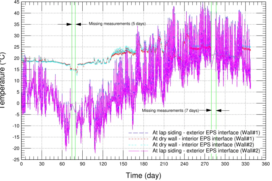
taken between the vinyl siding and the exterior EPS layer, on the face of the concrete behind the exterior EPS layer, on the face of the concrete behind the interior EPS layer, and between the drywall and the interior EPS layer. The measured temperatures at the vinyl siding – exterior EPS interface and at the drywall – interior EPS interface were taken as time dependent boundary conditions for solving the energy equation (Eq. (3)). These measured temperatures are shown for Wall#1 and Wall#2 in Figure 3 where time = 0 corresponds to October 13th at ~15:00. The measured temperatures for both walls at the vinyl siding – exterior EPS interface are approximately equal. At the drywall – interior EPS interface, however, these temperatures are approximately equal for both walls during the first period of the test and that for Wall#2 is to some extent higher than that of Wall#2 during the last period of the test (t > ~135 d). As shown in Figure 3, these temperature measurements were missing during two periods of 5 days (time = 74.3 d – 79.4 d) and 7 days (279.8 d – 286.8 d). In Numerical simulation, it was assumed that these temperatures changed linearly during these two periods (see Figure 3).

By considering the boundary conditions at vinyl siding – exterior EPS and drywall – interior EPS interfaces, there is no need to include both vinyl siding and drywall in the numerical simulations. In future work, however, numerical simulations will be conducted to investigate the transient response (including the effect of infiltration and exfiltration) of full-scale ICF wall assemblies subjected to different Canadian climates. The numerical simulation was conducted for a period of 337.67 d for both ICF walls. Since the boundary conditions for Wall#1 are close to that for Wall#2, the numerical results presented in this report are for Wall#1 only. The benchmarking of the present model against the experimental data and the transient response of the ICF wall are discussed next.

-25 -20 -15 -10 -5 0 5 10 15 20 25 30 35 40 45 0 30 60 90 120 150 180 210 240 270 300 330 360

At lap siding - exterior EPS interface (Wall#1) At dry wall - interior EPS interface (Wall#1) At dry wall - interior EPS interface (Wall#2) At lap siding - exterior EPS interface (Wall#2)

Missing measurements (7 days) Missing measurements (5 days)

Time (day)

Temper

ature (

o

C)

5 RESULTS AND DISCUSSIONS

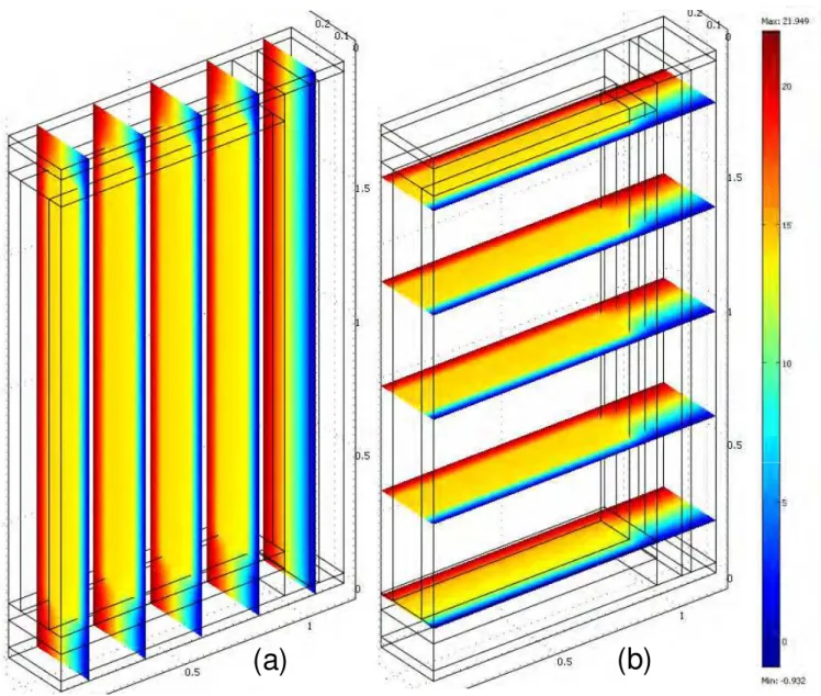
Figure 4 shows the temperature contours in five vertical and horizontal slices passing through the ICF wall at the end of simulation (time = 161.66 d). The first 4 vertical slices are passing through the ICF and the last vertical slice is passing through the wood frame on RHS of the ICF (Figure 4a). Figure 4 shows that the temperature distribution within the concrete layer is approximately uniform. Also, as shown in this figure, the wood frame in the mid-scale ICF assembly (see Figure 1) acts as thermal bridges due to its higher thermal conductivity (0.09 W/mK) compared to EPS (0.033 W/mK). A 3D thermal model is needed to predict the thermal performance of wall systems with window and door openings, corners, and structural joints with roofs, floors, ceilings and other walls, where the effect of thermal bridges cannot be neglected. Simplifying the problem to one dimensional can lead to errors in determining the energy efficiency of building envelope. However, for a clear/opaque ICF wall system (uninterrupted by wall details), the effect of these thermal bridges will be minimal, and the thermal performance can be accurately predicted by 1D thermal model.

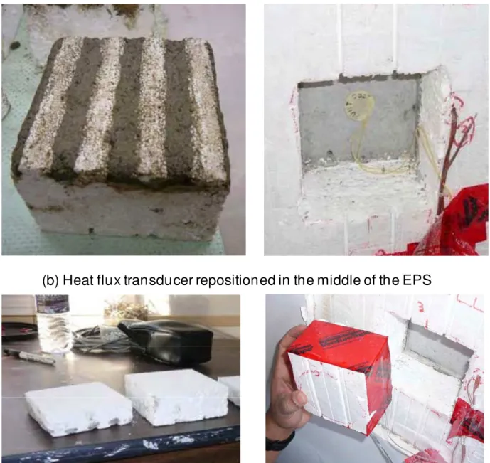
During the first three months of the experiment, two heat flux transducers were positioned at the EPS-concrete interfaces. This proved a complex task due to the grooves in the interior side of the foam. To provide a flat surface for the heat flux transducers so that the measured heat flux component is perpendicular to the surface, a section of foam was removed prior to pouring the concrete. The grooves in the removed section of the EPS were filled in with wet concrete and cured before the foam section was put back into position (see Figure 5a). By doing this, the heat flux transducer was neither exposed to a uniform material nor in good contact with the material – but rather alternating lines of foam and concrete on the heat flux transducer surface (forming fins from both foam and concrete materials) with trapped air voids. The combined effect of both the fins (specifically the concrete ones since it has high thermal conductivity, 1.4 W/mK, compared to EPS, 0.033 W/mK, see Table 1) with the trapped air voids (thermal conductivity = 0.025 W/mK), called “fins effect” could result in a different heat flux readings than the actual heat flux passing through the ICF assembly if the removed section of the foam shown in Figure 5a is in a good contact with the surface of concrete.

(a)

(b)

(a) Removed section of EPS foam for heat flux transducer installation

(b) Heat flux transducer repositioned in the middle of the EPS

Figure 5 Installation of heat flux transducer in the ICF test specimen.

When the measured heat fluxes were used to calculate the R-value of the ICF assembly during the periods of minimal change in the thermal environment (at pseudo steady-state conditions), it was found that the calculated R-value was R-14, which was much lower than the expected one (R~20). At this stage, it was decided to use the present model to interpret the results of the heat

flux measurements and to improve the experiment design by repositioning the heat flux transducers at different locations in the EPS layers.

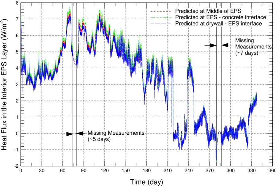
Figure 6 shows the predicted heat flux at different locations in the interior EPS layer at the wall center. As indicated earlier, time = 0 corresponds to October 13th at ~15:00. As shown in this figure, the differences between the predicted heat fluxes at drywall – interior EPS interface, at the middle of the interior EPS and at the interior EPS – concrete interface are small. The small differences between these heat fluxes are due to the small thermal mass of the EPS layer (see Table 1). Furthermore, when the predicted heat flux was used to calculate the R-value during the periods of pseudo steady-state conditions, the obtained R-value was approximately the same as expected for the ICF wall (R ~ 20).

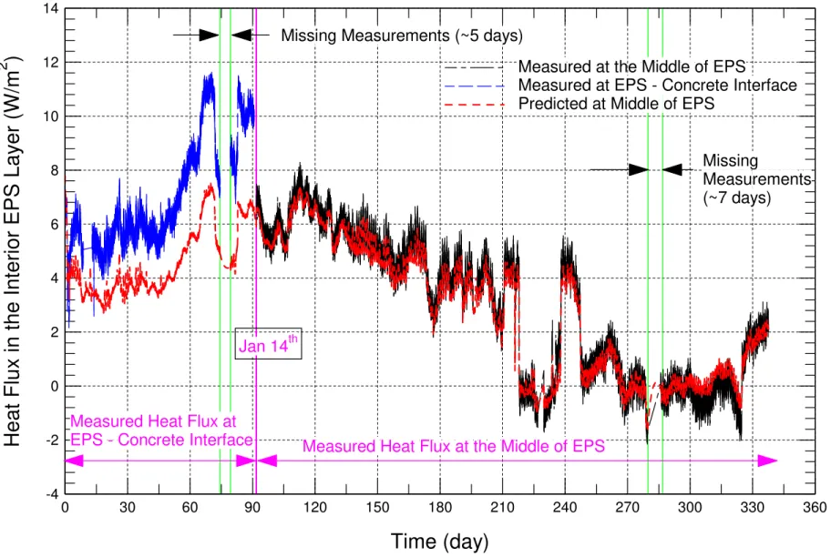
During the first three months of the experiment (October 13th to January 14th), the predicted heat flux at the middle of the interior EPS layer was compared with the measured heat flux at the interior EPS – concrete interface at the center of wall in Figure 7. As shown in this figure, the trends of both the measured and predicted heat fluxes with time are approximately the same. However, the measured heat flux was ~30% higher than the predicted one due to the fin effect as indicated earlier. Consequently, it was decided to expose the heat flux transducers that were installed at the exterior EPS – concrete interface and at the interior EPS – concrete interface to a uniform material by repositioning them between two blocks of foam (approximately at the middle of the EPS layers as shown in Figure 5b). By doing this, it was possible to expose the heat flux transducers to uniform material and to ensure that these heat flux transducers were in a good contact with the EPS material and with homogenous material. Full descriptions of the instrumentation of the experiment and test results will be reported at a later date. Thereafter, the predicted results using the present model were compared with the measurements. During the last period of the experiment (January 14th to March 24th, after repositioning the heat flux transducers), Figure 7 shows a comparison between the predicted and measured heat fluxes at the middle of the interior EPS layer. As shown in Figure 7, the agreement between the model prediction and experiment is reasonably good. Furthermore, the mean bias error and root-mean-square error between the model prediction and experiment were 0.235 W/m2 and 0.347 W/m2, respectively.

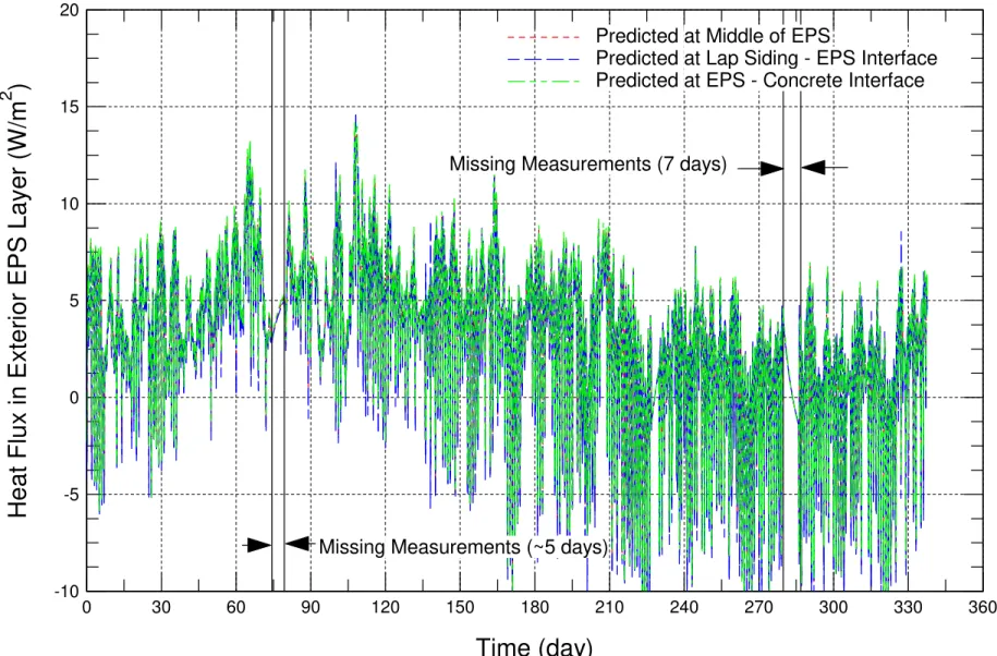
In the exterior EPS layer, Figure 8 shows a comparison between the predicted heat fluxes at the concrete – EPS interface, at the middle of the EPS and at the EPS – vinyl siding interface at the center of wall. As shown in this figure, the differences between the predicted heat fluxes at different locations are very small. Given that the EPS has a small thermal mass (see Table 1) and the temperature at vinyl siding – EPS interface changes significantly with time (see Figure 3), the exterior EPS layer has a fast thermal response. As such, the predicted heat fluxes in the exterior EPS layer change significantly with time (Figure 8).

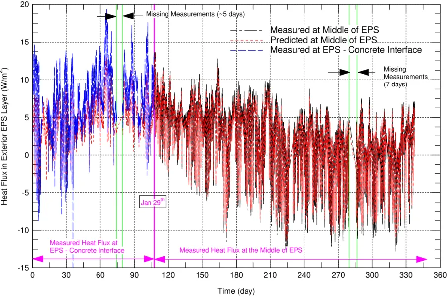
During the first period of the experiment from October 13th (day 0) to January 29th (day 108), the predicted heat flux at the middle of the exterior EPS layer is compared with measured one at the concrete – EPS interface in Figure 9 at the center of wall. Similar to the case of interior EPS layer, the measured heat flux was ~30% higher than the predicted one (e.g. see Figure 10 for a period of two weeks from day 56 to day 70). On January 29th (day 108), the heat flux transducer at the concrete – exterior EPS interface was repositioned at the middle of the exterior EPS (Figure 5b). During the last period of the test (January 29th to March 24th), Figure 9 shows a comparison between the measured heat flux at the middle of exterior EPS with the predicted one. The mean bias error and root-mean-square error between the model prediction and experiment were 0.126 W/m2 and 0.630 W/m2, respectively. Figure 9 shows the agreement between the model prediction and experiment is reasonably good.

A final step for benchmarking the present model was conducted by comparing its prediction for the heat flux at the vinyl siding – exterior EPS interface with the measured one at the center of wall. This comparison is shown in Figure 11. Despite the large scatter in measured heat flux at the vinyl siding – EPS interface during the last period of the test, Figure 11 shows that both predicted and measured heat fluxes are in good agreement. After gaining confidence in the present model, it was used to investigate the effect of thermal mass due to concrete layer on the thermal performance of ICF wall subjected to a Canadian climate conditions as presented next.

-2 -1 0 1 2 3 4 5 6 7 8 0 30 60 90 120 150 180 210 240 270 300 330 360

Predicted at Middle of EPS

Predicted at EPS - concrete interface Predicted at drywall - EPS interface

Missing Measurements (~7 days) Missing Measurements (~5 days)

Time (day)

Heat Flux in the Interior EPS Layer (W/m

2

)

-4 -2 0 2 4 6 8 10 12 14 0 30 60 90 120 150 180 210 240 270 300 330 360

Measured at the Middle of EPS

Measured at EPS - Concrete Interface Predicted at Middle of EPS

Missing

Measurements (~7 days)

Measured Heat Flux at the Middle of EPS Measured Heat Flux at

EPS - Concrete Interface Jan 14th

Missing Measurements (~5 days)

Time (day)

Heat Flux in the Interior EPS Layer (W/m

2

)

-10 -5 0 5 10 15 20 0 30 60 90 120 150 180 210 240 270 300 330 360

Predicted at Middle of EPS

Predicted at Lap Siding - EPS Interface Predicted at EPS - Concrete Interface

Missing Measurements (7 days)

Missing Measurements (~5 days)

Time (day)

Heat Flux in Exterior EPS Layer (W/m

2

)

-15 -10 -5 0 5 10 15 20 0 30 60 90 120 150 180 210 240 270 300 330 360

Measured at Middle of EPS Predicted at Middle of EPS

Measured at EPS - Concrete Interface

Missing Measurements (7 days) Missing Measurements (~5 days)

Measured Heat Flux at the Middle of EPS Measured Heat Flux at

EPS - Concrete Interface

Jan 29th Time (day) H eat Fl ux in Ex ter ior EPS Lay er ( W /m 2 )

0 5 10 15 20 56 57 58 59 60 61 62 63 64 65 66 67 68 69 70

Measured at Middle of EPS Predicted at Middle of EPS

Measured at EPS - Concrete Interface

Time (day)

Heat Flux in Exterior EPS Layer (W/m

2

)

-15 -10 -5 0 5 10 15 20 25 30 35 0 30 60 90 120 150 180 210 240 270 300 330 360 Predicted Measured Missing Measurements (7 days) Missing Measurements (~5 days) Time (day) H eat Fl ux at Lap Si di n g EPS Inter fa c e ( W /m 2 )

6 EFFECT OF THERMAL MASS

In order to quantify the contribution the thermal mass due to concrete layer on the energy savings, two walls were considered as shown in Figure 12. The first wall is an ICF wall similar to the tested wall as previously described with a concrete layer of 200 mm thick (Figure 12a). The second wall is similar to the ICF but without a concrete layer (Figure 12b). These walls were subjected to indoor conditions according to ASHRAE recommendation (ASHRAE 2003). Additionally, these walls were subjected to outdoor conditions obtained from weather data of Ottawa (wet year 1965). In these analyses, the effect of wind, cloud coverage, short wave solar radiation, and long wave solar radiation on the thermal performance were taking into consideration. The initial temperature of the entire wall assemblies of both walls was assumed uniform and equal to 10oC. The numerical simulations were conducted for a period of one year. In these analyses, the thermal performance were evaluated by taking into consideration the effect of heat transfer by natural convection in the air layer between the vinyl siding and the external EPS layer.

Figure 13a and Figure 13b show snapshots of the vertical velocity contours in the air layer at the end of simulations for ICF walls with and without concrete layer, respectively. Since the temperature at the air layer – exterior EPS interface is higher than that at vinyl siding – air layer interface, the air close to the EPS surface moves upward while the air close to the vinyl siding surface moves downward due to the bouncy effect (Figure 13). Note that when the present model was benchmarked against the experiment data (see the previous section), the vinyl siding, air layer and gypsum board were not considered in the numerical simulation because temperature boundary conditions (same as the measured temperatures given in Figure 3) were applied at the air layer – exterior EPS interface and at the drywall – interior EPS interface.

Figure 14 shows the predicted heat flux on the indoor surface of gypsum board in the cases of ICF walls with and without concrete layer. In this figure, positive heat flux represents the case when heating load is need while negative heat flux represents the case when cooling load is need. As shown in this figure, because of the effect of thermal mass of the concrete layer, the heat flux on the indoor surface of the gypsum board does not significantly fluctuate with time compared to

wall without concrete layer. Furthermore, the peaks of heat fluxes in the case of wall with concrete layer are always smaller than wall without concrete layer. As such, a home with walls with concrete layer would require a smaller size of the furnace (heating system) compared to a home with walls without concrete layer. This is one of the advantages of the effect of thermal mass due to concrete layer.

The positive and negative heat fluxes shown in Figure 14 were used to calculate the accumulative energy loss and accumulative energy gain, respectively. The obtained results are shown in Figure 15 through Figure 18. Figure 16 shows that the yearly accumulative energy losses from walls with and without concrete layer were 1224 W-day/m2 and 1296 W-day/m2, respectively. As such, the effect of thermal mass due to concrete layer resulted in an energy saving in the heating load of ~6% compared to wall without concrete layer. Also, Figure 18 shows that the yearly accumulative energy gain in the case of wall with concrete layer (2 W-day/m2) is much lower than that in the case of wall without concrete layer (37 W-day/m2). Consequently, the effect of thermal mass due to concrete layer contributed in reducing the cooling load compared to the case without concrete layer. Note that for a cold climate such as Ottawa weather, the yearly accumulative energy gain (contributed in the cooling load, see Figure 16) in the cases of walls with and without concrete layer are much smaller that the yearly accumulative energy loss (contributed in heating load, see Figure 18). Future work will be conducted to investigate the effect of thermal mass of ICF wall systems on energy savings (both heating and cooling loads) when these walls are subjected to cold and hot climate conditions of North America. The outcome of this work will be reported at a later date.

Conc

re

te

(200

m

m

t

h

ic

k)

E

P

S

(63.5 m

m

t

h

ic

k)

E

P

S

(63.5 m

m

t

h

ic

k)

E

P

S

(63.5 m

m

t

h

ic

k)

E

P

S

(63.5 m

m

t

h

ic

k)

G

y

ps

um

(12.7 m

m

t

h

ic

k)

G

y

ps

um

(12.7 m

m

t

h

ic

k)

V

inyl

s

idi

ng

Ai

r

V

inyl

s

idi

ng

Ai

r

(a) ICF Wall

_{(b) ICF Wall without concrete}

(a) ICF Wall

(b) ICF Wall without concrete

Figure 13. Snapshot of the vertical velocity contours (in mm/s) in the air layer between vinyl siding and external EPS layers at the end of simulation

-4 -2 0 2 4 6 8 10 0 30 60 90 120 150 180 210 240 270 300 330 360 390

Indoor Surface (Without Concrete) Indoor Surface (With Concrete)

Require Cooling Load Require Heating Load

Time (day)

Heat Flux (W/m

2

)

0 100 200 300 400 500 600 700 800 900 1000 1100 1200 1300 0 30 60 90 120 150 180 210 240 270 300 330 360 390

Wall With Concrete Wall Without Concrete

Time (day)

Cum

u

lative Energy Loss

(i.e

. Re

qu

ire

He

at

ing Load) (W.day/m

2

)

Wall

 With Concrete

Wall

 Without Concrete

Series1

1224

1296

1180

1200

1220

1240

1260

1280

1300

1320

Ye

a

rl

y

 Cu

m

u

lati

v

e

 En

e

rg

y

 Lo

ss

 (W

.d

ay

/m

)

0 5 10 15 20 25 30 35 40 0 30 60 90 120 150 180 210 240 270 300 330 360 390

Wall With Concrete Wall Without Concrete

Time (day)

Cumulative Energy Gain

(i.e. Require Cooling Load) (W.day/m

2

)

Wall

 With Concrete

Wall

 Without Concrete

Series1

2

37

0

5

10

15

20

25

30

35

40

Ye

a

rl

y

 Cu

m

u

lati

v

e

 En

e

rg

y

 Gai

n

 (W

.d

a

y

/m

)

7 SUMMARY AND CONCLUSION

This study and a number of other studies (Elmahdy et al., 2009, Saber et al., 2010a and 2010b, 2010c, 2010d, Saber and Swinton, 2010, Saber et al., 2011a and 2011b, 2011c) were conducted to benchmark the NRC-IRC’s hygrothermal model, called hygIRC-C. This model solves simultaneously the 2D and 3D Heat, Air and Moisture (HAM) transport equations. In this study, no moisture transport was taken into consideration. During the first period of the test, the readings of the heat flux transducers that were positioned at the EPS-concrete interfaces were used to determine the value of the ICF test specimens. It was found that the calculated R-value during the periods of pseudo steady-state conditions (i.e. during the periods of minimal change in the thermal environment) was much lower than the expected R-value. The present model was then used to interpret the results of the heat flux measurements and to improve the experiment design by repositioning the heat flux transducers at different locations in the EPS layers. As a result of the small thermal mass of the EPS, the numerical results showed that the differences between predicted heat fluxes at different locations in each EPS layer were small. As such, it was decided to reposition these heat flux transducers at the middle of the EPS layers. Thereafter, the numerical results were compared with the measurements. The results showed that the comparison between the present model predictions and experimental data was reasonably good.

After the present model was benchmarked, it was used to quantify the contribution of the thermal mass due to concrete layer of ICF wall system when it was subjected to the climate conditions of Ottawa. Results showed that the thermal mass due to concrete layer resulted in an energy saving in the heating load of ~6% compared to wall without concrete layer. This research is on-going. The present model will be used to conduct numerical simulations in order to investigate the transient thermal response of full-scale ICF wall assemblies subjected to different cold and hot climate conditions of North America. The results of this effort will be the subject for future publications.

8 REFERENCES

ASHRAE. 2009. 2009 ASHRAE Handbook –Fundamentals (SI). 26.5. Atlanta: American Society of Heating, Refrigerating, and Air-Conditioning Engineers Inc.

ASHRAE Handbook – Applications, Chapter 3 – Commercial and Public Buildings, Atlanta: American Society of Heating, Refrigerating and Air-Conditioning Engineers, Inc., 2003. ASTM Designation: C 518-04, Steady-State Thermal Transmission Properties by Means of the

Heat Flow Meter Apparatus, Section 4, Volume 04.06, Thermal Insulation, 2007 Book of ASTM Standards.

ASTM Designation: C 1130-07, “Standard Practice for Calibrating Thin Heat Flux Transducers”, Annual Book of ASTM Standards, sec 4, Construction, vol 04.06, Thermal Insulation; Building & Environment Acoustic, pp. 577-584, 2009.

Bird, R.B., Stewart, W.E., and Lightfoot, E.N. 1960. Transport Phenomena, John Wiley & Sons, Inc., pp. 149-150.

Burch, D.M., W.L. Johns, T. Jacobsen, G.N. Walton, and C.P. Reeve. 1984a. “The Effect of Thermal Mass on Night Temperature Setback Savings.” ASHRAE Transactions, 90(part 2), 184-206.

Burch, D.M., K.L. Davis, and S.A. Malcomb. 1984b. “The Effect of Wall Mass on the Summer Space Cooling of Six Test Buildings.” ASHRAE Transactions 90 (part 2), 5-21.

Burch, D.M., D.F. Krintz, and R.F. Spain. 1984c. “The Effect of Wall Mass on Winter Heating Loads and Indoor Comfort—An Experimental Study.” ASHRAE Transactions 90 (part 1), 94-114.

Christian, J.E. 1991. “Thermal Mass Credits Relating to Building Energy Standards.” ASHRAE Transactions 97 (part 2), 941-957. Christian, J.E., J. Kosny, A.O. Desjarlais, and P.W. Childs. 1998. “The Whole Wall Thermal Performance Calculator–On the Net.” In Proceedings, Thermal Performance of the Exterior Envelopes of Buildings VII, 287-299. Atlanta, Ga.: American Society of Heating, Refrigerating and Air-Conditioning Engineers. Christian, J.E., J. Kosny, A.O. Desjarlais, and P.W. Childs. 1998. “The Whole Wall Thermal

Performance Calculator–On the Net.” In Proceedings, Thermal Performance of the Exterior Envelopes of Buildings VII, 287-299. Atlanta, Ga.: American Society of Heating, Refrigerating and Air-Conditioning Engineers.

COMSOL Multiphysics, version 3.5a, www.comsol.com.

Elmahdy, A.H., Maref, W., Swinton, M.C., Saber, H.H., and Glazer, R. 2009-b. Development of energy ratings for insulated wall assemblies. Building Envelope Symposium, San Diego, California, October 26, 2009, pp. 21-30.

Environment Canada, 2010. Canadian Climate Normals 1971-2000, Ottawa MacDonald Cartier International Airport [online]. Available from: http://www.climate.weatheroffice.gc.ca [accessed 18 March 2010].

Gajda, J., 2001. Energy Use of Single-Family Houses with Various Exterior Walls. Research & Development Information Report. Portland Cement Association and Concrete Foundations Association. PCA CD026. PP 1-46.

Hersh Servo AG. 2010. Insulated Concrete Forms [online]. Available from: http://www.hirsch-gruppe.com [accessed 29 April 2010].

Hill, D. and Monsour, R., Monitored Performance of an Insulating Concrete Form Multi-Unit Residential Building, Draft Final Report, prepared by Enermodal Engineering Limited, www.enermodal.com, September 2006.

Kosny, J., E. Kossecka, A.O. Desjarlais, and J.E. Christian. 1998. “Dynamic Thermal Performance of Concrete and Masonry Walls.” In Proceedings, Thermal Performance of the Exterior Envelopes of Buildings VII, 629-643. Atlanta, Ga.: American Society of Heating, Refrigerating and Air-Conditioning Engineers.

Kosny, J., T. Petrie, D. Gawin, P. Childs, A. Desjarlais and J. Christian. 2001. “Energy Benefits of Application of Massive Walls in Residential Buildings.” In Proceedings, Performance of Exterior Envelopes of Whole Buildings VIII, Session IX-A. Atlanta, Ga.: American Society of Heating, Refrigerating and Air-Conditioning Engineers.

Kossecka, E., and J. Kosny. 1998. “Effect of Insulation and Mass Distribution in Exterior Walls on Dynamic Thermal Performance of Whole Buildings.” In Proceedings Thermal Performance of the Exterior Envelopes of Buildings VII, 721-731. Atlanta, Ga.: American Society of Heating, Refrigerating and Air-Conditioning Engineers.

Maref, W., Kumaran, M.K., Lacasse, M.A., Swinton, M.C., and van Reenen, D. “Laboratory measurements and benchmarking of an advanced hygrothermal model”, Proceedings of the 12th International Heat Transfer Conference, Grenoble, France, August 18, 2002, pp. 117-122 (NRCC-43054).

NAHB Research Center 1999, “Insulating Concrete Forms: Comparative Thermal Performance” prepared for U.S. Dept. of Housing and Urban Development. August 1999.

Petire, T., Kosny, J., Desjarlais, A., Atchley, J., Childs, P.W., Ternes, M.P. and Christian, J., 2001, “How Insulating Concrete Form vs. Conventional Construction of Exterior Walls Affects Whole Building Energy Consumption: Results from a Field Study and Simulation of Side-by-Side Houses”

Rabin, Y., and Rittel, D. “A Model for the Time Response of Solid-embedded Thermocouples”, Experimental Mechanics, VoL 39, No. 2, pp. 132-136, 1999.

Saber, H.H., Maref, W., Elmahdy, A.H., Swinton, M.C., and Glazer, R. “3D Thermal Model for Predicting the Thermal Resistances of Spray Polyurethane Foam Wall Assemblies”, Building XI conference, Clearwater, Florida, 2010a.

Saber, H.H., Maref, W., Lacasse, M.A., Swinton, M.C., and Kumaran, K. “Benchmarking of Hygrothermal Model against Measurements of Drying of Full-Scale Wall Assemblies” International Conference on Building Envelope Systems and Technologies, ICBEST 2010, Vancouver, Canada, June 27-30, 2010b.

Saber, H.H., Maref, W., and Swinton, M.C. “Thermal Response of Basement Wall Systems with Low Emissivity Material and Furred Airspace” Submitted for Publication to the Journal of

Building Physics, December, 2010c.

Saber, H.H., Maref, W., Armstrong, M.M., Swinton, M.C., Rousseau, M.Z., and Ganapathy, G., "Benchmarking 3D Thermal Model against Field Measurement on the Thermal Response of an Insulating Concrete Form (ICF) Wall in Cold Climate", Eleventh International

Conference on Thermal Performance of the Exterior Envelopes of Whole Buildings XI

(Clearwater, FL, USA, December 4-9, 2010d).

Saber, H.H., Swinton, M.C. “Determining through Numerical Modeling the Effective Thermal Resistance of a Foundation Wall System with Low Emissivity Material and Furred – Airspace” International Conference on Building Envelope Systems and Technologies, ICBEST 2010, Vancouver, Canada, June 27-30, 2010.

Saber, H.H., Maref, W., Elmahdy, H., Swinton, M.C., and Glazer, R. “3D Heat and Air Transport Model for Predicting the Thermal Resistances of Insulated Wall Assemblies”, International Journal of Building Performance Simulation,

(http://dx.doi.org/10.1080/19401493.2010.532568), First published on: 24 January 2011a (iFirst), pp. 1-17.

Saber, H.H., Maref, W., Swinton, M.C., and St-Onge, C., "Thermal analysis of above-grade wall assembly with low emissivity materials and furred-airspace," Journal of Building and

Environment, volume 46, issue 7, pp. 1403-1414, 2011b

(doi:10.1016/j.buildenv.2011.01.009).

Saber, H.H, and Laouadi, A. “Convective Heat Transfer in Hemispherical Cavities with Planar Inner Surfaces (1415-RP)” Accepted for Publication to the Journal of ASHRAE Transactions, March 2011c.