Autonomous Error Bounding of Position
Estimates from GPS and Galileo
by
Thomas J. Temple
Bachelor of Arts in Computer Science and Engineering-Physics
Dartmouth College 2003
Submitted to the Department of Aeronautics and Astronautics
in partial fulfillment of the requirements for the degree of MASSACHUS, •iSN,,
OF TECHNOLOGY
Master of Science in Aeronautics and Astronautics
iNOV 0 2 2006
at the
MASSACHUSETTS INSTITUTE OF TECHNOLOGY
LIBRARIES
September 2006
@
Thomas J. Temple 2006. All rights reserved.
The author hereby grants to MIT permission to reproduce and
distribute publicly paper and electronic copies of this thesis document
in whole or in part.
A uthor
...
... -.
w .
-r
. ..- . ...Department of Aeronautics and Astronautics
August 24, 2006
Certified by ...
... ....
Jonathan P. How
Accepted by...
Associate Professor
DA4Iautiautics and Astronautics
S..
...
.
..aime
Perair...
Jaime Peraire
Professor of Aeronautics and Astronautics
Chair, Committee on Graduate Students
Autonomous Error Bounding of Position Estimates from
GPS and Galileo
by
Thomas J. Temple
Abstract
In safety-of-life applications of satellite-based navigation, such as the guided approach and landing of an aircraft, the most important question is whether the navigation error is tolerable. Although differentially corrected GPS is accurate enough for the task most of the time, anomalous measurement errors can create situations where the navigation error is intolerably large. Detection of such situations is referred to as integrity monitoring. Due to the non-stationary nature of the error sources, it is impossible to predetermine an adequate error-bound with the required confidence. Since the errors at the airplane can be different from the errors at reference stations, integrity can't be assured by ground monitoring. It is therefore necessary for the receiver on the airplane to autonomously assess the integrity of the position estimate in real-time.
In the presence of multiple errors it is possible for a set of measurements to remain self-consistent despite containing errors. This is the primary reason why GPS has been unable to provide adequate integrity for aircraft approach. When the Galileo system become operational, there will be many more independent measurements. The more measurements that are available, the more unlikely it becomes that the errors happen to be self-consistent by chance. This thesis will quantify this relationship. In particular, we determine the maximum level of navigation error at a given probability as a function of the redundancy and consistency of the measurements.
Rather than approach this problem with statistical tests in mind, we approach this as a machine learning problem in which we empirically determine an optimal mapping from the measurements to an error bound. In so doing we will examine a broader class of tests than has been considered before. With a sufficiently large and demanding training data, this approach provides error-bounding functions that meet even the strictest integrity requirements of precision approaches.
We determine the optimal error-bounding function and show that in a GPS + Galileo constellation, it can meet the requirements of Category I, II and III precision approach-a feat that has proven difficult for GPS alone. This function is shown to underestimate the level of error at a rate of less than 10-7 per snapshot regardless of the pseudorange error distribution. This corresponds to a rate of missed detection of
less than 10- 9 for all approach categorizations. At the same time, in a 54 satellite constellation, the level of availability for Category I precision approaches availabil-ity exceeds 99.999%. For Category II and III precision approaches, it can provide availability exceeding 99.9% with either a 60 satellite constellation, or with a modest improvement over existing LAAS corrections.
Contents
1 Introduction 13
1.1 M otivation . . . . 14
1.1.1 Integrity of a Position Estimate . ... 14
1.1.2 Current Approach .... ... .... . . 16 1.1.3 Previous Difficulty ... 16 1.1.4 Research Context ... 18 1.2 Problem Statement ... 19 1.2.1 Unknown Error ... 20 1.2.2 Discrete Decisions ... 20
1.2.3 Continuous Error Bounds . ... . 21
1.2.4 Under-Estimation of Error . ... . 22
1.3 Thesis Outline . ... .. ... .. . .. . . . .. .. . . . 25
2 Problem Formalism for Precision Approaches 27 2.1 Objective Function ... 27
2.1.1 Discrete Classification . ... ... 28
2.1.2 Minimum Expected Cost ... .. 29
2.2 Algorithm Design ... 30
2.2.2 Algorithmic Framework ... 32 2.2.3 Scatter ... ... .. 33 2.2.4 Geometric Considerations ... ... . 34 2.2.5 Metrics ... 39 2.2.6 W eights, 3 . . . .. . . . . 41 2.2.7 Scale, a(k) . . . . 41 3 Methodology 43 3.1 Search . . . .. . 43 3.1.1 Sum m ary ... 43 3.1.2 Subset Size . . . .. . . . . 44 3.1.3 Scale Topology ... 45 3.1.4 W eight Topology ... 47 3.1.5 Norm s . . . 48 3.1.6 M odel Order ... 48 3.2 Simulation Environment ... 49 3.2.1 Error M odel ... 50 3.2.2 Size Limitations ... 52 4 Results 55 4.1 Search Results ... 55
4.1.1 Optimal Subset Size ... 55
4.1.2 Number of Metrics ... 60
4.1.3 N orm s . . . 61
4.1.4 Weights ... 61
4.1.5 Scale . . . 66
4.3 Validation Results ...
5 Conclusions 75
List of Figures
1-1 Error-Bound outcomes ... 22
1-2 Empirical Pseudorange Error Distribution . ... 24
2-1 CDFs of Vertical Error and DOP Adjusted Vertical Error ... 36
3-1 Scatter-plot of Single Metric and Error . ... 46
3-2 Experimental Range Error ... 51
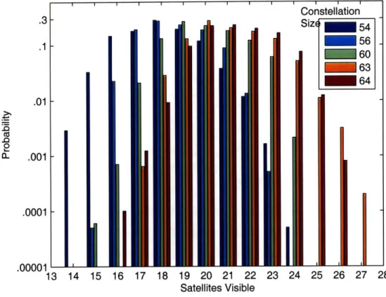
4-1 PDF of Number of Satellites Visible . ... 56
4-2 Performance by Subset Size ... .... 58
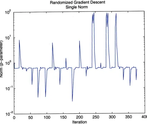
4-3 Convergence of Single-Metric Search . ... 62
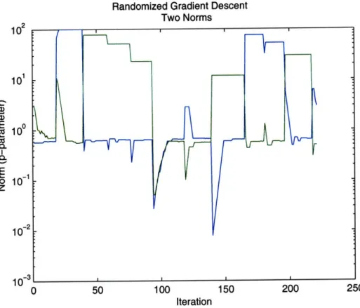
4-4 Convergence of Two-Metric Search . ... 63
4-5 Convergence of Three-Metric Search . ... 64
4-6 Level of Service Availability by Norm . ... . . . 65
4-7 Performance by Satellites Visible . ... . . . . 67
4-8 Optimal Scaling Factors ... 68
4-9 Progression of Optimal Scaling Factors . ... 70
List of Tables
1.1 Precision Approach Categories ... ... 15
1.2 Outcome Classifications ... 21
3.1 Search Components ... ... ... . . 44
4.1 Precision Approach Integrity Requirements . ... 71
4.2 Category I False Alarm Rates ... ... 74
Chapter 1
Introduction
Imagine yourself as an airplane pilot approaching a runway surrounded in fog. You must rely on your navigational instruments for your position relative to the runway. You don't need to know the exact position of the airplane; as long as the airplane is within some predetermined safe region, say, within x meters of a nominal 30 glide-slope, you can be confident that you will land safely. You would like to be very confident that you are within that region.
You have a number of measurements from different sensors available to you and when you consider them all, you can estimate that you are within the safe region. You have enough sensors so that the there is some redundancy. Under what conditions would you abort the landing?
1. All 5 sensors agree almost exactly.
2. All 22 sensors agree almost exactly.
3. Some of the 5 sensors disagree substantially.
Clearly, closer agreement is more appealing and more sensors are preferable to fewer. One can make that determination without regard to the error distribution from which the sensor readings were drawn. The goal of this thesis is to quantify this intuition. The key idea is that the larger the number of measurements, the more representative they become of the distribution from which they were selected and the less reliant we need to be on assumptions regarding the a priori distribution.
1.1
Motivation
1.1.1
Integrity of a Position Estimate
In order to use a Global Navigation Satellite System (GNSS) for navigation, it must meet the users' requirements for accuracy, availability and integrity. The availability of the system is the fraction of the time that the system is deemed safe to use for a particular application while the integrity is the ability of the system to protect against errors. More specifically, the integrity is defined as the probability that a position error of a given magnitude will be detected. There is a trade-off between availability and integrity, e.g., one can trivially provide perfect integrity at zero availability.
In safety-of-life applications integrity is of the utmost importance. Suppose that a GNSS system meets the accuracy requirements of an application nearly all time, but ins some rare cases, say, one in a million estimates, the level of inaccuracy puts lives in danger. If the system is unable to identify most of those cases, it cannot be used. This is the situation in which the differentially corrected GPS finds itself today in the application of precision approach.
A precision approach is one in which both vertical and horizontal guidance are used to acquire the runway. In this thesis we will only focus on the vertical component of the guidance since it is more demanding. Typically, if the runway is not visible from
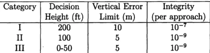
Category Decision Vertical Error Integrity
Height (ft) Limit (m) (per approach)
I 200 10 10
-II 100 5 10-9
III 0-50 5 10- 9
Table 1.1: Integrity requirements for precision approach. These requirements are still under discussion within the aviation community.
a height of 700-1000 feet above the runway (depending on the obstruction around the airport), then the pilot must receive horizontal and vertical guidance to descend lower. Such approaches are called precision approaches.How low the airplane can descend on instruments depends on the pilots training and the plane's avionics. There are three categories of precision approaches numbered I, II and III with Category III subdivided in to IIIa, b and c for very low decision heights. These have increasingly exacting requirements as the airplane gets closer to the runway as shown in Table 1.1. If the runway is not visible from the decision height, the landing is aborted.
Currently, precision approaches in the United States require the Instrument Land-ing System (ILS), which provides of a set of radio beams aligned with the glide slope, or angle of approach, of the landing airplane. The ILS is more expensive than a GPS solution since it requires installation and maintenance of precise equipment at every runway end. Local differential correction would only require one signal for the entire airport and would be cheaper than a single ILS beacon. The ILS is scheduled to begin phase-out in 2015[3].
The integrity required for precision approach is given in Table 1.1. Despite high-hopes and a truly astonishing level of accuracy, differential GPS is finding it a chal-lenge to meet the strict integrity requirement[ 11].
1.1.2
Current Approach
In GPS, the task of providing integrity has been handled by a receiver function called receiver autonomous integrity monitoring (RAIM). There are two different ways of approaching RAIM depending on whether temporal information is also considered, which divides RAIM techniques into "snapshot" and "filtered" techniques. snapshot techniques attempt to determine the degree of agreement among the measurements and generally use various least-squares statistical methods. Filtered algorithms gen-erally use some form of Kalman filter, which requires knowledge of temporal error covariances. Filtered algorithms are also typically based on least-squares estimation. In this thesis we will concentrate on snapshot techniques because it relies less heavily on knowing a priori the nature of the error. However, we will reconsider whether
least-squares is the best approach for assessing integrity.
A diverse group of snapshot RAIM algorithms have been proposed based on vari-ous methods of detecting and quantifying the disagreement among the measurements.
These methods vary in the way measurements are compared and they vary in the test statistic used to assess those comparisons. This thesis seeks to resolve these differ-ences empirically. In particular, we propose a space of error-bounding algorithms that includes practically all existing snapshot RAIM methods as well as yet uncon-sidered algorithms of similar form. We then employ search algorithms to determine the error-bounding algorithm that we expect to perform the best in terms of integrity and availability.
1.1.3
Previous Difficulty
The difficulty in detecting multiple errors of similar magnitude results from the possi-bility that the errors may be self-consistent. For instance if every measurement were the correct pseudorange to the same (although in incorrect) position, they would
agree perfectly although there would still be error. To be more precise, let p denote the a vector of the pseudorange measurements. The position equations are linearized which makes the position estimate, ý, the solution to the over-constrained system of linear equations[18]
p = G~.
Where G is called the geometry matrix and it's rows are the cosines of direction of the satellite from the position estimate in the local reference frame.1 This is commonly solved using the least-squares fit.
x = (G'G)-1G'p
Let p = p + e where 3 is the true measurement and E is the error. Let 2 denote the true position.
&
= (G'G) -
1
G'( + e)
S- x = (G'G) -'G'E (1.1)
Now consider the residuals.
p - G. = (I - G(G'G)-'G')p
= (I - G(G'G)-
1G')( + e)
= (I
-
G(G'G)-'G')(Ga + e)
= (G(I
-
I)J + (I
-
G(G'G)-1G')e
= (I - G(G'G)-
1
G')E
(1.2)
Suppose that e = Gb for some vector b.
S- = (G'G)-'G'Gb = b
p - G- = (I - G(G'G)-iG')Gb = (G - G)b = 0
The residuals are zero while the position error is precisely b. This case is intractable. Our only chance is for such an arrangement of errors to be extremely unlikely. For this to happen, e must lie in the span of the columns of G, which is k x 4, where k is the number of satellites visible. As k increases, it becomes more and more unlikely that such an event will occur. Or more accurately, it becomes increasingly unlikely that the errors will be close to the span of G. With a single constellation where it is common to have 7 or fewer satellites visible, this probability is simply unmanageable for safety-of-life applications. However with the much larger constellation provided by GPS + Galileo, the probability will decrease to a manageable level.
1.1.4
Research Context
Originally, snapshot methods consisted of an algorithm to determine if one of the satellite ranges was faulty[19]. "Faulty" in this context meant grossly erroneous.
But as pointed out in [14], for the application of precision approach, detecting single satellite "faults" is not enough. In the information rich environment provided by the combined GPS + Galileo constellations, gross faults will be stand out obviously and the differential reference stations will reliably detect them. We will instead concern ourselves with a metric notion of the quality of the ranges as a whole as is done in [5]. An intuitive approach is to define a test statistic based on a measure of the dis-agreement among the measurements and define a threshold for that statistic below which the system is declared safe to use. Most of the existing techniques take this
ap-proach, including [8-10, 17, 20], some of which employ search to determine optimality. Fundamentally, the same approach is taken here. In particular, the algorithm space explored in this thesis is considered to be a generalization of [17]. However, we would like to make a conceptual distinction.
We adopt the change of focus introduced in [5], moving from the discrete notion of faults to a metric notion of quality, specifically maximum error at a given proba-bility. Instead of focusing on a test statistic and application-specific thresholds, we will instead provide a set of quality metrics and a function that maps them to a safe error-bound. If we can show the mapping to be reliable, it can be used more generally since it does not require any application specific parameters, e.g., thresh-olds and error models. In practice, the algorithm could be used "out of the box" without consideration of signal environment; it will be equally reliable on corrected or uncorrected, filtered or unfiltered ranges. In particular, one would be free to ex-clude measurements using traditional RAIM before handing those measurements to the error-bounding algorithm.
1.2
Problem Statement
Rather than detect faults per se, our goal is to allow an airplane's GPS receiver to place an upper-bound on the error in its position estimate obtained from a set of pseudorange measurements. Primarily we require the probability that the true error is greater than the bound be very small, thereby ensuring integrity. Given that, we would like the upper-bound to be tight, i.e., under-estimate as little as possible, to
1.2.1
Unknown Error
A difficulty comes from the fact that we don't know enough about the pseudorange
errors a priori. We don't know how they correlate temporally which will require that the error-bound be determined in real-time, i.e., based only on the "snapshot" of cur-rent sensor readings. Nor do we adequately know their distribution. This will cost a great deal of analytical traction. We will treat this issue by analyzing error-bounding
algorithms using simulated data. This data will include realistic as well as extremely challenging pseudorange error distributions. Finally, we don't know the spacial co-variances between pseudorange errors from different satellites. Fundamentally, this is intractable-if the only information available is from the sensors and the sensors are allowed to collude to hide as discussed in Section 1.1.3, nothing can be done. For this thesis we will assume the pseudorange errors in measurements from different satellites to be independent.
1.2.2
Discrete Decisions
In the precision approach problem, the aviation community has designated an "alert limit" on position error that it considers to be the limit of safety. If the Integrity Monitor can only choose to raise an alarm or not, that dictates four discrete scenarios (see Table 1.2). If true error was greater than the alert limit and we raised the alarm we will call that a "correct detection" and if we failed to raise the alarm a we will call it a "missed detection". If the true error was less than the alert limit and we raised the alarm we will call that a "false alarm," while the cases in which we do not raise an alarm will be referred to as "service available". For each scenario there are relative costs and allowable rates of occurrence. This specification defines an optimization problem, in particular we want to find the algorithm that is most likely to satisfy it.
algo-Error Tolerable Error Intolerable Alarm Raised False Alarm Correct Detection Alarm Not Raised Service Available Missed Detection Table 1.2: The possible outcomes of raising, or not raising, an alarm.
rithm. The ellipse represents a scatter-plot of the results of running a particular algorithm on a data set. If we replaced "error bound" with "test statistic" on the abscissa, this would be a traditional threshold setting problem. In such a problem we would be looking for the vertical line that segments the data with minimum cost. In our approach however, the threshold is not a free parameter, instead it is held fixed at the value given in the specifications. Pictorially, rather than moving the threshold, we can move and reshape the data by changing the error-bounding algorithm. For instance, simply by scaling the algorithm one can segment the data in any way that a threshold could. But by changing the algorithm in other ways we can perhaps change the shape of the distribution to a more favorable one.
1.2.3
Continuous Error Bounds
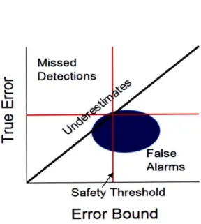
The discrete notions of false alarms and missed detections are somewhat incompatible with the continuous notion of an error-bound. For instance in Figure 1-1 there are data-points in which the error-bound under-estimates although those points are in the "Service Available" or "Correct Detection" region. But clearly with a different threshold, the classification of any one of these points could be changed to a missed detection. This enforces an intrinsic notion of scale which is antithetical to our goal of avoiding assumptions regarding the measurement error distribution. To avoid this, we will map the discrete notions of missed detections and false alarms to the continuous notions of error-bound under- and over-estimates.
W L.. o Missed Detections
y>
7~~
Alarms
Safety ThresholdError Bound
Figure 1-1: Scatter-plot of error/error-bound pairs for a particular algorithm on a data set.
1.2.4
Under-Estimation of Error
Instead of promising a certain level of missed detections, we will promise a certain level of under-estimates. All missed detections are also under-estimates. Based on our empirical knowledge of the measurement error distribution, we can put an upper bound on the fraction of over-estimates that could be missed detections. This ap-proach gives us a great deal of traction in dealing with a largely unknown pseudorange error distribution.
For example, suppose we have enough real world data to confidently say that a particular error model, for instance a Gaussian mixture, is a good description of the pseudorange error in 99% of snapshots. Suppose that we can show analytically that the fault rate for this error distribution is practically nil. This tells us that a missed detection is only possible 1% of the time. This is sometimes referred to as the "unconditional fault rate". Suppose also that we can show analytically or in
simulation that our algorithm underestimates only 0.01% of the time for an arbitrary distribution. Finally if we can show that whether our algorithm under-estimates or not is independent of the size of the true error, then we can claim a 0.0001% rate of missed detections.
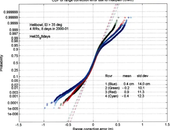
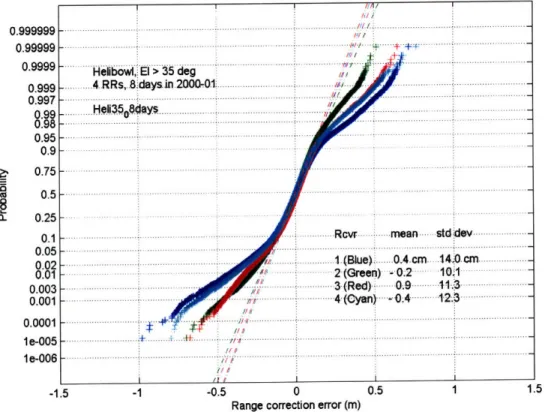
Figure 1-2 shows the cumulative probability distribution function (CDF) of pseu-dorange error for a real receiver using local differential corrections. The errors are of a completely tolerable magnitude in every case. However, there aren't enough cases to prove adequate integrity. Furthermore, the experiment was conducted it a single location. However, at this location at least, a Gaussian mixture could describe at least 99.9% of the data very well.
Similarly, we can use empirical data to determine the mapping from over-estimates to false alarms. However, the false alarm rate doesn't need to be known to as extreme a precision as the missed detection rate. This means that we are free to determine false alarm rate based on actual empirical data or more conveniently an idealized model of it.
CDF of range correction error due to multipath (CMC) - h/i 4 Helibowii b jo-vs; EI > 3 5 d e g - 4... ..RRs,..8idays in.2000.1 " H...ei 35.8d
.-
.
y.s....... .
... ..
.
.
... . . .:::: ::: :.... .... .. ... .. ...- ... -.... ... ... - Rcvr mean std d-a
... ... ... ... ... ... ... .. ... .. ... ... ... ... ... ... ... ... .... .. .. ... ... . ... .... ... ... - 2 (Green) -0.2 10.1 -i 3( Red) 0.9 11.3 - 4 (cyan) -0.4 12.3-w
+ 2-Gep- 10.1 i -i cm...Range correction error (m)
Figure 1-2: Empirical distribution of pseudorange error after applying a local dif-ferential corrections from four different reference stations. A Gaussian mixture, for instance O.9fN(O, 0.10m) + 0.1N(0, 0.30m), is a very good representation of this dis-tribution. (Courtesy: FAA technical Center, Atlantic City, NJ)
0.999999 0.99999 0.9999 0.999 0.997 0.99 0.98 0.95 0.9 0.75 0.5 0.25 0.1 0.05 0.02 0.01 0.003 0.001 0.0001 le-005 le-006 -1.5 I ~ ~~~ r ¸
...
...
..
..
I
..
.
I
...
.
...
...
..
...
...
ý
I
...
...
...
... I i//, •1.3
Thesis Outline
The goal of this thesis is to determine the best algorithm for placing an error-bound on the position estimate of an airplane executing a precision approach. This work is arranged as follows. Section 2.1 quantitatively defines the notion of performance by which we will judge algorithms. Section 2.2 defines the space of algorithms we will consider. Chapter 3 poses the search problem and discusses the methodology
and algorithms for conducting it. Section 4.1 discusses the results of the search with the optimal algorithm given by Equation 4.4. The best algorithm found is then validated in Section 4.3. We conclude in Chapter 5 that these results demonstrate the adequacy of this algorithm for all categories of precision approaches. Finally, Section 5.1 discusses the implications of this work.
Chapter 2
Problem Formalism for Precision
Approaches
In this chapter, we pose the problem of determining the best algorithm to generate error-bounds from a snapshot of pseudoranges as a non-linear optimization problem. In Section 2.1 we quantitatively define our objectives and in Section 2.2 we define the space of algorithms that fall under consideration. In Chapter 3 we describe how this space is searched for the algorithm that optimizes our choice of objective function.
2.1
Objective Function
We are trying to find an algorithm that can determine whether or not it is safe to continue with an approach. If we treat this as a discrete decision and also treat safety as binary, the four cases in Table 1.2 are exhaustive and mutually exclusive-we only need to specify three of the four rates to fully describe the performance of an algorithm. Furthermore, the algorithm has no control over whether the true error is greater or less than the alert limit. This allows us to characterize performance by
specifying only two of these.
We seek to maximize the time when the landing service is available while keeping the missed detection rate below a mandated level, which we will denote T. Since the error rate is fixed, minimizing false alarms is equivalent to maximizing availability in our context. Let us approach the problem as a non-linear optimization problem. Let A denote the space of all error bounding algorithms.
objective : arg min P(False Alarm)
aEA
such that : P(Missed Detection) < T (2.1)
2.1.1
Discrete Classification
Suppose that we have a large and representative data set of n measurement-error pairs, (mi, ei). Then a good approximation to Problem 2.1 would be to replace the probabilities with their maximum likelihood estimates. Let FA, MD, SA and CD denote zero-one functions defined over errors and error bounds that indicate whether a particular event is a false alarm, missed detection, service available or correct detection, respectively. Let
PFA ZFA(a(mi), ei)
1n i=1 PMD n 1 MD(a(mi), D ei) i=1 n n i=l PCD = 1- CD(a(m1), e1) i=1
making the problem
objective : such that :
arg min PFA
aEA
PMD < T.
(2.2)
But it might not be prudent to suppose that the missed detection rate is zero simply because we haven't had a missed detection yet. We could instead be Bayesian and use artificial counts to represent a uniform prior probability distribution. This would make the estimates used in problem 2.2
1 PFA -n+l 1 PMD = -n+l PSA - 1 n+l PCD = -n+1 ( + FA(a(m), ei)) 1 + MD(a(m2), ei) 1 + SA(a(m1), ei)
1 +
CD(a(m),
ei).
i= 1We can convert Problem 2.2 into an unconstrained optimization problem using a barrier or penalty function. Instead we take a slightly less artificial tack.
2.1.2
Minimum Expected Cost
If we assign a relative cost, c, to each of the four possible outcomes, we can pose the problem as minimum expected cost.
(2.4)
arg min (CMD ' PMD + CFA " PFA + CSA ' PSA + CCD ' PCD)
aEA
The rate at which errors of unsafe magnitude occurs is fixed, let it be, Pe. We can rewrite Objective 2.4 as
arg min (CMD ' PMD + CFA ' PFA + CSA(1 - Pe - PFA) + CCD(Pe - PMD)) aEA
or
arg min (PMD(CMD - CCD) + PFA(CFA - CSA) + constants)
aEA
Since the optimization is unaffected by a linear function, we can subtract out the
constant terms and divide by CFA - CSA.
Defining C CMD - CCD
CFA - CSA
we have
arg min (C -PMD + PFA) (2.5)
aEA
It should be noted that Problems 2.1 and 2.5 are not the same. Solving 2.5 will not ensure that the constraint on missed detections is met. Instead it will balance the
rate of missed detections appropriately against the rate of false alarms. We must decide in the end whether or not the result is satisfactory.
2.2
Algorithm Design
2.2.1
Future Data
The primary problem is that it is impossible to obtain a data set on which to assess the probabilities in Equation 2.5. What we want is a data set that is representative of future conditions. Since the missed detection rate is to be kept extremely low, it would require an unrealistic level of prescience to acquire a data set that would let
us predict the probabilities with sufficient accuracy. Clearly we're going to have to make some sort of assumptions about the kind of data that we're going to see.
Suppose that we have enough empirical knowledge to say that at least some frac-tion of the time, 7, the measurement error will conform to some nominal distribufrac-tion, N. Let's assume that the measurement errors within a pseudorange snapshot are inde-pendent and identically-distributed (IID). At the same time, this implies that there is another, unknown distribution, X, from which the errors are drawn 1- T of the time. Either analytically or numerically, we can determine the performance of an algorithm on errors from N and for particular choices of X. For instance we might suppose that X is
+1
meter uniform error and that N is 0.9NA(0, 0.14m) + O.lA(0, 0.42m). But notice that empirically we can say relatively little about the validity of this choice of X. For instance, suppose that we define a new distribution Y = yX for some scalar 7, making Y = ±Tym uniform. It is impossible to say whether we should consider X or Y when analyzing an error-bounding algorithm. In fact, the errors are non-stationary. They might conform to X some of the time and Y the rest.This leads us to an important feature of the algorithms that we will consider. We will attempt to make the algorithm robust to the scale of the error. Let p = fi + E
where #f is the vector of true pseudoranges and c is the vector of pseudorange errors. The least squares solution to the position equations is given by
x = (G'G)-1G'p
(G'G)-'G'3 + (G'G)-'G'6
since (G'G)-1G'p is the true position, then the position error is simply (G'G)-1G'c which is a linear function of e. That is to say if we replaced ei with yiE the position error would become -yei. Therefore we would like our error-bound to scale to 7£i.
a linear function of the range error. Furthermore the position error is a linear function of the residuals. Similarly, any least squares position computed from subsets of the ranges will move from the true position linearly. This implies that the distance between such position estimates will also scale.
2.2.2
Algorithmic Framework
To ensure that the space of algorithms is manageable, let us break the error-bounding algorithm into separate components. For a snapshot method, the only information available to the algorithm is
* the pseudorange measurements, p, and * the geometry matrix, G
Implicitly we have one more piece of information, the number of satellites visible, k. We will examine algorithms of the form
Error Bound = a(k) .METRICS(SCATTER(p,G)) (2.6)
Where
Scatter is intended to be suggestive of the disagreements among the measurements. The Scatter function maps the measurements into a set on the real line
Metrics characterizes the "spread" of the scatter by extracting a vector of the n most informative features of that set,
0
is a normalized vector of n weights assigning relative importance to the different metrics and,2.2.3
Scatter
Misra and Bednarz [17] originally introduced the notion of scatter. They proposed that one collect a number of subsets of j satellites each and compute a position estimate for each such subset. Then by comparing the solutions we can estimate the degree of inconsistency in the system. Here we use essentially the same methodology. Primarily, we would like to determine the best choice j.
For a subset of size four or greater, we compute the least squares position estimate for that subset and compare it to the position estimate using all the satellites. For a subset of size less than four, we first compute the position estimate for the excluded satellites and then compute the residuals from that position to the pseudoranges from the small subset. By analogy, we will consider the ordinary residuals as estimates for a subset size of zero.
Two natural choices for the number of satellites to use per subset are k - 1 and 1, i.e., the leave-one-out cross-validation estimates and the residuals to those estimates. This would mean that k subsets would clearly be sufficient seeing as that is be all of the subsets possible. For other choices, there will be a much larger number of subsets available.
First note that, while there are j-choose-k different subsets that we could choose, we are still solving a set of k linear equations. Regardless of the number of subsets used, there are only k independent measurements. This implies that all the positions computed will be a linear combination of some k position subset, with the relation dictated by the G matrix. This suggests that it might not be necessary to choose a large number of subsets.
It would be unwise to choose the satellite subsets randomly. Such randomness inevitably leads to over- and under-emphasis of certain satellites and can lead to disagreement going unnoticed. Although we will still choose satellites randomly, we
will mitigate this affect by including each satellite in the same number of subsets. Misra and Bednarz divided the sky into bins to determine which satellites would be included in subsets. This is problematic because a statically positioned bin will occasionally have only a small number of measurements in it, overemphasizing them. It is also very difficult to dynamically choose bins to avoid this. The reason for the bins was to avoid poor geometry subsets.' Here we avoid bad geometry by requiring the VDOP of a subset be bellow a predefined threshold. The impact of this threshold is mitigated by making certain adjustments to the scatter as will be discussed in Section 2.2.4.
To determine how many satellites to use per subset we compute the optimal single metric algorithms for each subset size of a fixed number of visible satellites. This is done for every subset size and for the ordinary residuals. For each we need to determine the norm to use and the scaling factor by which that norm is converted into an error bound. This is essentially a brute force search of a simplified space. It was not computationally realistic to consider multiple-metric algorithms while determining the best notion of scatter. Furthermore, while it would be possible to mix norms of wholly different notions of scatter, to consider this possibility the scale of the search would have to be considerably expanded.
2.2.4
Geometric Considerations
From the geometry matrix one is able to determine how the measurements interrelate. We will use the geometry information to adjust the scatter to reflect our confidence due to the interrelation of the measurements.
First and simplest, the covariance of the position estimate is proportional to
1
The quality of the geometry is given by (G'G)- 1. The square-root of the sum of the diagonal of
this matrix is referred to as the "dilution of precision" or DOP, while the square-root of the third element of the diagonal is referred to as the "vertical dilution of precision", or VDOP.
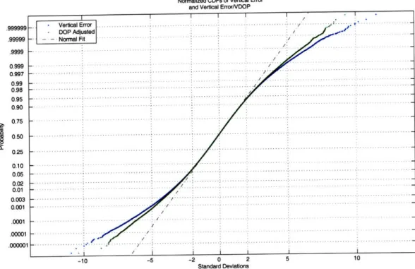
(G'G)-1[18]. It seems obvious then that we should scale the scatter by the VDOP of all the satellites in view. Figure 2-1 shows how such a correction tightens the CDF of the error. Even though it is a relatively small change, it is an important improvement-accounting for uncertainty in the position estimate due to the geom-etry.
If we compute the position estimate (using all the satellites) and then compute a estimate using a subset, we can determine the position that would be computed from the opposite subset that is it's exclusion simply by examining the geometry. Let S, and S, be two subsets of satellites that are mutually exclusive and collectively exhaustive, i.e., every satellite is included in exactly one of the subsets. Let G,, Gb be the rows of G corresponding to Sa, Sb respectively with zeros in the rows corresponding to satellites from the other subset. The position estimates are given by
xa = (G1Ga) -1Gap
Xb =
(G'Gb)-1G'b
Rearranging and summing we have(G'Ga)Xa + (G'Gb)xb = G'p + G'p
Since G = Ga + Gb
(GaG,)xa + (GbGb)xb
=
G'p
The overall estimate, x is given by x = (G'G)- 1 = G'p so,
Normalized CDFs of Vertical Error and Vertical ErrorNDOP
.999999 .99999 .9999 0.999 0.997 0.99 0.98 0.95 0.90 0.75 0.50 0.25 0.10 0.05 0.02 0.01 0.003 0.001 .0001 .00001 .000001 -5 -2 0 2 Standard Deviations
Figure 2-1: Normalized CDFs of vertical error and vertical error divided by VDOP. The pseudorange errors were selected from a Gaussian mixture. Normalization en-sures that both distributions have zero mean and unity covariance. The VDOP adjusted error has tighter tails, indicating that vertical error divided by VDOP is a "better behaved" variable3 than vertical error. Although the curves only deviate in the extreme ends of the tails, we are trying to predict extreme behavior and the tightness of the tails is our primary concern.
I I ·. - I -. - -V4N - D .. . . . ..- . . . . .- . . . . . .. ..- . . .. ..- . . -I. .... ... .. . ... .... q ... ... ... ... ... ... ... ... ...
which expands to
(G'Ga)Xa + (G2Gb)xb = ((Ga + Gb)'(Ga + Gb))x
xb = (GbGb)-1(((Ga + Gb)'(Ga + Gb))X - (G'aGa)a)
Zb
=
x+
(GGb)
-(GCGa) (x
-
Xa) + (G'Gb + GIGa)•
.
Note that Ga and Gb have complimenting zeros making the mixed terms zero. This lets us conclude the following relationship.
Zb - X = (G(Gb)-1(GaGa)(X - Xa) (2.7)
The difference between the position estimate and an estimate based on a subset of the satellites is linearly related to the difference between the position estimate and the estimate based on the subset acquired by excluding those satellites. The relation is given by Equation 2.7. We can use this result to adjust the scatter such that there becomes no difference between a subset of size j and one of k - j. This result does not rely on the invertability of (G'Ga), except for the implicit definition of Xa. If (GaGa) is not full rank, we can replace (G'Ga)xa with G'p giving us
xb
-
x
= (G'Gb)-
1(G1Ga)X
-
Gap.
(2.8)
In particular, G' could consist of a single row, making G'p a single directed pseudorange, while Xb would then be the leave-one-out solution. This corresponds to
Lee's famous result [13] showing the equivalence of residual and position comparison techniques. More importantly for our purposes, this proves that subset positions differences and pseudorange residuals are functionally equivalent in that they both scale linearly with position error.
The amount of disagreement between two position estimates is a vector, while we have defined scatter as a set of scalars. We will simply project this vector on the direction that we care about-the vertical. If we were concerned with the magnitude of position error in general, we could take its norm instead. Analogously, the residuals can be considered to be directed in that they point towards a satellite. Somewhat surprisingly however, because of the first term in Equation 2.8, they don't necessarily move the estimate in that direction. Nonetheless we can determine their direction of influence and likewise project this direction against the vertical.
Suppose that a satellite subset has a bad geometry. That suggests that it will estimate a position far from the overall estimate, even if the pseudoranges are rela-tively consistent. Bad subset geometry will exaggerate the disagreement between the measurements. In the overall estimate, bad geometry will increase the error bound while a bad subset geometry will make us less confident that the disagreement exists.
In the case of residuals, an analogue to the above is not immediately obvious. We would like to know how "susceptible" the position estimate is to influence from the satellite whose residual we are considering.4 For illustration, imagine that all of the satellites lie in a plane except one: if we compute a position by excluding the range from the out-of-plane satellite, the residual for the out-of-plane satellite could be extremely large. We correct for this with the a notion of "directed DOP" of the estimate.
Directed DOP - Ga(G'bGb)1/2 (2.9)
4This "susceptibility" is very close to the notion of "slope" presented in [8]. It is different in
that slope determines how much of the pseudorange error appears in the estimate while here we are concerned with how much the pseudorange error will appear in the residual.
Making the ith adjusted residual
(Gaix - pi)Gai(G'Gb)12e3
0
0
where e3s is the direction of interest.
1 07
For symmetry, the DOP adjustment for position scatter was changed to also be "directional" in the same sense. That is to say we proceeded with
(Zb - x)'(GIGb)1/2e3
rather than
(Xb - x)e3(e'(G'Gb)-le3)- 1/2
It should be noted that this is not the only means by which this adjustment could be pursued. We found this method to work better than using the slope in [8] or ordinary DOP. We suspect that this is due to better utilization of information in the off-diagonal terms of G'G and (G'G)- 1
2.2.5
Metrics
To ensure a manageable space to search, we must predefine a space of metrics. Since scatter scales appropriately, any function of the scatter that scales linearly would also scale. For example, with a fixed number of measurements, the standard deviation would scale appropriately. Let S denote the scatter set. Consider the following
functions.
l1 = exp (ZESilog(s) (2.10)
17 = (k-4)ES IsP) (2.11)
loo = max IsI (2.12)
sES
Function 2.10 and 2.12 are the limits of Function 2.11 as p approaches 0 and oo respectively. We will refer to these functions as "norms" although for p less than one, they do not obey the triangle inequality. Also the normalization term, k - 4, makes it appear that we are going to compare the norms of sets with different cardinalities, which would break the vector space on which the norms are defined. This is not strictly true since the algorithm is conditioned at the top level by the number of satellites visible. This term is simply a constant that can be absorbed by the scale function a(k). It is only included here in the hope of later simplifying the form of
A probability distribution becomes increasingly well described by an increasing number of it's moments[15]. The fact that these norms are isomorphic to moments, suggests that the set of 2.10 through 2.12 are sufficiently descriptive representation of the scatter. In particular, we expect some finite (preferably small) subset of them to form an adequate description for estimating the magnitude of the error. As such, the problem of determining the optimal metrics consists of finding the optimal set of p-parameters.
2.2.6
Weights, /
If we map the measurements and position errors (p, G, E) to the space, S, defined by
S - (METRICS(SCATTER(p,
G)),
e),then the remainder of the algorithm, i.e., a and fl, is simply a hyperplane separating over- and under-estimates. Because of the requirement that our prediction be robust to the scale of the error, all these hyperplanes must pass through the origin. We will allow there to be different hyperplanes depending on the number of satellites visible but to avoid having a large number additional parameters we will require that they all be the same in the subspace that is S with the errors removed. The weights, i
chooses the most informative "side" of the the measurements in this subspace. To be conservative about over-fitting this plane to a small feature specific to the data set, we will require that all of the weights be non-negative. This has the important side effect of drastically reducing the number of local minima in the space of weights.
2.2.7
Scale, a(k)
Conceptually, the scale function distinguishes the error-bounding approach from an ordinary test statistic. Although 0 times the metrics is a test statistic, we have taken pains to ensure that it scale linearly with error. At this point we simply provide a constant factor to relate our statistic to worst case position error at a given probability. We have yet to address the central question of how to account for the number of measurements, i.e., the number of satellites visible, k. The algorithm clearly should consider the number of measurements available. It would be possible to use this information to condition the algorithm at the innermost level. We could use a different
number of metrics with different norms and weights for every different number of satellites we can see. We could even use different scatter functions. The benefit (and also the price) for doing so would be that there would be a larger number of free parameters in the overall algorithm (for instance the number of p-parameters would go from n to kn). More parameters allow the algorithm to more tightly bound the error in the training data. At the same time, the more parameters we have, the less well this improved performance will generalize to future data. Since performance on future data is of utmost importance, we should only introduce new parameters where it is substantially beneficial to do so.
So where is the natural place to condition on the number of satellites visible? In this work we will place it in the absolute scaling. Primarily because it introduces the fewest free parameters if it is inserted at that point. We do not expect the particular norms are the most informative about scatter to be sensitive (or at least not overly sensitive) to the number of points making up the scatter distribution. Intuitively, one would expect additional measurements to translate directly into additional confidence. To mitigate the risk of over-fit, we will enforce this intuition, requiring that the absolute scaling be monotone decreasing as more measurements are made available.
It may be the case that the most informative norms stay the same but their relative importance varies. This would recommend conditioning on the number of measurements at the relative weighting point. If this were the case we would expect a large degree of continuity between weights of neighboring numbers of measurements. We assume that the optimal relative weights change slowly (if at all) with varying numbers of measurements available.
Another reason to keep the influence of k at the top level is that a(k) encapsulates the additional confidence we get from having more measurements available. This is a valuable thing in and of itself. Armed with this function, system designers would know exactly how much additional confidence would be provided by an additional signal.
Chapter 3
Methodology
Section 3.1 describes the methodology that was employed to search the space of algo-rithms defined in Section 2.2 for the one which minimizes Objective 2.5. Section 3.2 describes the data on which algorithms are to be evaluated. The results of this search are presented in Section 4.1.
3.1
Search
3.1.1
Summary
Recall that we are looking the algorithm that solves
arg min (C -PMD + PFA) (3.1)
aEA
Wherein A is the set of algorithms of the form
Error Bound = a(k) -/ -METRICs(SCATTER(p,G)) (3.2)
where PMD and PFA are the Bayesian estimates described in Equation 2.3. The value used for C is 107 to be consistent with our strict demands on missed detection rate.
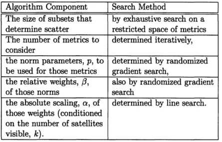
The algorithm space, A, can be defined by a relatively small set of parameters which are enumerated in Table 3.1. We will search this parameter space to determine the best algorithm. The rest of this section is devoted to discussing the types of search used to determine these parameters which are summarized in Table 3.1.
Algorithm Component Search Method
The size of subsets that by exhaustive search on a determine scatter restricted space of metrics The number of metrics to determined iteratively, consider
the norm parameters, p, to determined by randomized be used for those metrics gradient search,
the relative weights, 3, also by randomized gradient
of those norms search
the absolute scaling, a, of determined by line search. those weights (conditioned
on the number of satellites
visible, k).
Table 3.1: Components of the search
3.1.2
Subset Size
We will determine the size of subsets to use for scatter by determining the optimal algorithm for every subset size and then comparing their performance. Computation-ally, it is impractical to determine optimal algorithms for every subset size using the entire algorithm space and an adequately large data set. Therefore this portion of the search is restricted to single-metric algorithms.
3.1.3
Scale Topology
To determine how best to search for optimal weights and scale, we must carefully consider the topology of the objective function. If it is convex, or even quasi-convex we should be able to easily find its minimum. Conversely if it is highly non-convex we will have to be more judicious about how we conduct the search.
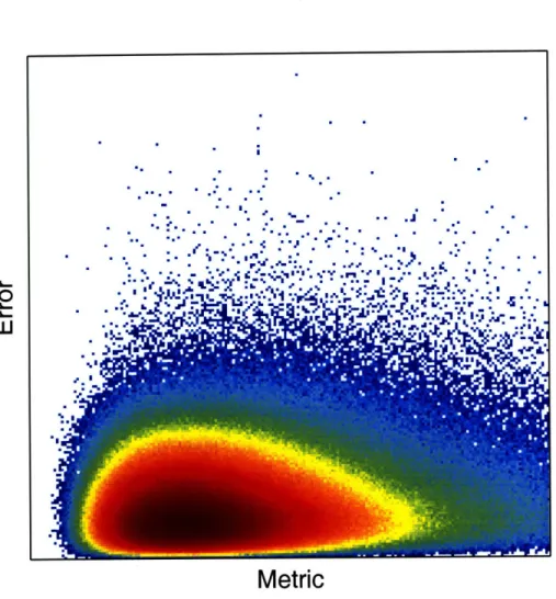
Given a set of metrics, the space of weights is a convex space. First consider all of the data in the space S in which each data point (p, G, ei) is plotted
(METRICS(SCATTER((p, G), ei).
For example, for a particular one-dimensional metric function, the results of this mapping is shown in figure 3-1. Assume for the moment that we have so much data that we can treat it as a continuous density and assume further that this density is convex in the space S. Since the error-bound is a convex function of metrics and we've assumed the the metrics are a convex density over our data, then the density of error/error-prediction pairs is convex for any choices of a and f.
Let O(a) denote the objective function 2.5. Given a particular METRICS function and fixed 3, we can define a new objective function O'(a).
O'(a) = O(a)
such that: a = a . 3. METRICS
For an individual data point, the objective is quasi-convex in a, i.e., it has a point about which the function is non-decreasing above and below. This is because on the one hand as a decreases, the bound tightens until it is no longer a false alarm, but at some point it becomes an under-estimate. The result of integrating a quasi-convex function over the convex density is quasi-convex[16]. Considering the entire data set,
0 L.= 3. 3 3. 3· C 3. 3. . . . • ." . ..:.--,....'- . • .'". ." - e L ,..=. .=. .· .j , -LC =
Metric
Figure 3-1: Scatter-plot of a data set of 5 million snapshots mapped into the met-ric/error space, S, for a particular one-dimensional metric function. Roughly speak-ing, the density is convex except at the fringe.
O'(a) is also quasi-convex.
But this is based on the assumption that the the measurement/error pairs have a continuous density. However, our data are discrete. This means that O'(a) isn't necessarily quasi-convex. However, in practice, the scale over which O' varies is very large with respect to the distance between points. For the contrary to be the case, one would have to squeeze more than 10' false alarms between two consecutive missed detections. In practice, this only happens at or near the global optimum. For finding the optimum weights given relative weights, the problem is quasi-convex, allowing an efficient solution using line search.
3.1.4
Weight Topology
Even with a continuous density of data, we are not assured that the objective function is convex over the space of weights. That is to say that
0"(3) =sup O(a)
such that a = a -,3 METRICS
is not quasi-convex. This is because the quasi-convexity of convolution only holds in one dimension[16]. Despite this lack of guarantee, if the gradient of O", VO",
changes slowly we can still find an optimum.
But discrete data also means that V#O" is undefined. We can get around this by estimating a gradient by examining nearby points. To use this gradient, the con-tinuity assumption needs to be examined more closely. One might expect that at fine resolution, level sets of O"(,) will be very jagged since they will follow
indi-vidual data points along the boundary. At a rougher resolution however, 0" varies smoothly with 3. We proceed by smoothing the gradient and employing standard
randomization techniques-those being to follow the empirical gradient from many randomly chosen starting points and to allow the search randomly move contrary to the gradient.
3.1.5
Norms
Given a fixed number of norms to use, we can attempt to find the particular ones that perform the best. This has as a sub-problem, the problem of finding the best weights and scale for each set of norms. The norms are continuous in their p-parameter as defined in Equation 2.11. This lets us define an empirical gradient by varying these parameters.
In this search, all bets are off in terms of favorable topology. It is unrealistic to hope that the outcome is sensitive to these parameters in a smooth way. To accom-plish this non-convex optimization we also use the empirical gradient and randomized search.
3.1.6
Model Order
We must also decide on the number of metrics to use. Since the class of (n+ 1)-metric algorithms includes the space of n metric algorithms (e.g., by setting one weight to zero) these define a set of nested hypothesis classes. We will begin by finding the best single metric algorithm. Then we will search for the best algorithm after adding a second metric. We will continue adding metrics until either performance levels off or the problem becomes computationally intractable.
Our ability to perform the gradient smoothing discussed in Section 3.1.4 is de-pendant on having a lot of data nearby. But data naturally spread out in higher dimensional spaces. Also, computing many empirical gradients becomes increasingly costly. This will put pressure on the number of metrics we will be able to consider at
a time. This is compounded by the fact that we are most interested in fringe cases that represent rare but large errors.
A more important reason to limit the dimensionality is the risk of over-fit. Since we are optimizing over a maximum likelihood estimate, we should not expect actual performance to be entirely commensurate with the performance on the training data. Even if we are to use a less optimistic estimator, the risk of over-fit continues. If the algorithm is allowed too much freedom, it can pick out features that are peculiar to the training data and not indicative of future data.
3.2
Simulation Environment
To generate the data on which this search will be performed, we simulate a suite of constellations and randomly chosen user positions. The constellations are Walker n/m/1 with m denoting the number of satellites, between 42 and 64, divided between m evenly spaced orbital planes. The third Walker parameter is the phase between satellites in adjacent planes and is equal to 3600/n. The elevation and inclination are equal to those of the GPS constellation. The simulated user is positioned randomly (uniform by area, not by lat/lon) between the arctic and antarctic circles. The time is chosen uniformly within one period of the constellations orbit.
To save on computational overhead, each constellation is used for 10 geometry snapshots (i.e., time). Each of these geometry snapshots is used for 10 user positions. For each of these positions, different pseudorange errors are generated. A satellite is considered "visible" if it is more than 5 degrees above the horizon.
Pseudorange errors are drawn independently from a predefined error model and the user estimates his position using the ordinary least squares solution to the position equations.' The error between this estimate and the users actual position is considered
the true error, 9.
3.2.1
Error Model
The data set consists of two parts, a false-alarm data set and a missed detection (or rather under-estimation) data set. Since the rate of false alarms does not need to be known to such a high level of certainty, it is relatively small and has its pseudorange errors drawn from a realistic nominal distribution. The missed detection data set on the other hand is much larger and has pseudorange errors drawn from a very pessimistic distribution.
The error model used to determine false alarm rate is based on the empirical data in Figure 3-2. This is represented by a Gaussian mixture drawing from mean zero, standard deviation 14cm 90% of the time and from m mean zero standard deviation of 42cm 10% of the time (which we will write as 0.9K (0, 0.14m)+0.1K/(0, 0.42m)), which is only modestly conservative. This mixture relationship is a common representation of the realities of multipath. It is important to note that the fact that the distribution is mean zero is inconsequential because all the bias ends up in the receiver clock.
The error model used for determining under-estimation rate is uniform. Since the algorithm is designed to be invariant to the scale of the distribution, the width of the distribution is irrelevant and set arbitrarily to ±1 meter.
The uniform distribution was found by [17] to be the most challenging. Most over-bounding distributions (e.g., [10,21]) although they are pessimistically wide, their tails still fade like a Gaussian and this provides traction. It is worth noting that this distribution is not necessarily the most pessimistic one possible. For a particular constellation, time and receiver position, there will be worse distributions possible. Such a distribution would introduce range errors in such that they correspond to a
position estimate even while we use other methods to assess that fit. This is to avoid risking the creation of a new source of bias.