The biogeochemistry and residual mean circulation of the southern ocean

(1)

The biogeochemistry and residual mean

circulation of the Southern Ocean

by

Takamitsu Ito

Submitted to the Department of Earth Atmospheric and Planetary

Sciences

in partial fulfillment of the requirements for the degree of

Doctor of Philosophy

at the

MASSACHUSETTS INSTITUTE OF TECHNOLOGY

Feburary 2005

( Massachusetts Institute of Technology 2005. All rights reserved.

I

A uthor ...

...

Depart

nt of Earth Atmospheric and Planetary Sciences

'~~~~~1

~October

7, 2004

Certified by..

John C. Marshall

Professor

Thesis Supervisor

Accepted by ...

.. .

Maria Zuber

Department Head, Department of Earth, Atmospheric and Planetary

Sciences

, . -...

APR 14

25 I

IL

.JI

LIBRARIES

'C/ .. k J

(2)

(3)

-The biogeochemistry and residual mean circulation of the

Southern Ocean

by

Takamitsu Ito

Submitted to the Department of Earth Atmospheric and Planetary Sciences on October 7, 2004, in partial fulfillment of the

requirements for the degree of Doctor of Philosophy

Abstract

I develop conceptual models of the biogeochemistry and physical circulation of the Southern Ocean in order to study the air-sea fluxes of trace gases and biological pro-ductivity and their potential changes over glacial-interglacial timescales. Mesoscale eddy transfers play a dominant role in the dynamical and tracer balances in the Antarctic Circumpolar Current, and the transport of tracers is driven by the residual mean circulation which is the net effect of the Eulerian mean circulation and the eddy-induced circulation.

Using an idealized, zonally averaged model of the ACC, I illustrate the sensitivity of the uptake of transient tracers including CFC11, bomb-Al4C and anthropogenic

CO2 to surface wind stress and buoyancy fluxes over the Southern Ocean. The model

qualitatively reproduces observed distribution of CFC11 and bomb-Al4C, and a suite of sensitivity experiments illustrate the physical processes controlling the rates of the oceanic uptake of these tracers. The sensitivities of the uptake of CFC11 and bomb-A14C are largely different because of the differences in their air-sea equilibration timescales. The uptake of CFC11 is mainly determined by the rates of physical transport in the ocean, and that of bomb-A14C is mainly controlled by the air-sea

gas transfer velocity. Anthropogenic CO2 falls in between these two cases, and the

rate of anthropogenic CO2 uptake is affected by both processes.

Biological productivity in the Southern Ocean is characterized with the circum-polar belt of elevated biological productivity, "Antarctic Circumcircum-polar Productivity Belt". Annually and zonally averaged export of biogenic silica is estimated by fitting the zonally averaged tracer transport model to the climatology of silicic acid using the method of least squares. The pattern of export production inferred from the inverse calculation is qualitatively consistent with recent observations. The pattern of inferred export production has a maximum on the southern flank of the ACC. The advective transport by the residual mean circulation is the key process in the vertical supply of silicic acid to the euphotic layer where photosynthesis occurs. In order to illustrate what sets the position of the productivity belt, I examined sim-ulated biological production in a physical-biogeochemical model which includes an

(4)

explicit ecosystem model coupled to the phosphate, silica and iron cycle. Simulated patterns of surface nutrients and biological productivity suggest that the circumpolar belt of elevated biological productivity should coincide with the regime transition be-tween the iron-limited Antarctic zone and the macro-nutrients limited Subantarctic zone. At the transition, organisms have relatively good access to both micro and macro-nutrients.

Kohfeld (in Bopp et al.; 2003) suggested that there is a distinct, dipole pattern in the paleo-proxy of biological export in the Southern Ocean at the LGM. I hy-pothesize that observed paleo-productivity proxies reflect the changes in the position of the Antarctic Circumpolar Productivity Belt over glacial-interglacial timescales. Increased dust deposition during ice ages is unlikely to explain the equatorward shift in the position of the productivity belt due to the expansion of the oligotrophic re-gion and the poleward shift of the transition between the iron-limited regime and the macro-nutrient limited regime. I develop a simple dynamical model to evaluate the sensitivity of the meridional overturning circulation to the surface wind stress and the stratification. The theory suggest that stronger surface wind stress could intensify the surface residual flow and perturb the position of the productivity belt in the same sign as indicated by the paleo-productivity proxies.

Finally, I examined the relationship between the surface macro-nutrients in the

polar Southern Ocean and the atmospheric pCO2. Simple box models developed in

1980s suggests that depleting surface macro-nutrients in high latitudes can explain

the glacial pCO₂ drawdown inferred from polar ice cores. A suite of sensitivity

ex-periments are carried out with an ocean-atmosphere carbon cycle model with a wide range of the rate of nutrient uptake in the surface ocean. These experiments suggest that the ocean carbon cycle is unlikely to approach the theoretical limit where "pre-formed" nutrient is completely depleted due to the dynamics of deep water formation. The rapid vertical mixing timescales of convection preclude the ventilation of strongly nutrient depleted waters. Thus it is difficult to completely deplete the "preformed" nutrients in the Southern Ocean even in a climate with elevated dust deposition in

the region, suggesting some other mechanisms for the cause of lowered glacial pCO2.

Thesis Supervisor: John C. Marshall Title: Professor

(5)

Acknowledgments

I would like to acknowledge John Marshall and Mick Follows for their guidance and support throughout my study at MIT. I also thank the thesis committee members, Ed Boyle, Kerry Emmanuel and Julian Sachs for their insightful comments for the thesis project, and I thank the climate modeling community at MIT for the development of MITgcm. I thank Bob Key for motivating the CFC11-bomb A14C relationship in the Southern Ocean (chapter 2), and Stephanie Dutkiewicz and Payal Parekh for the development of the global ocean physical-biogeochemical model, and Samar Khatiwala and Francois Primeau for motivating the matrix formulation of the tracer transport (chapter 3).

Physical oceanography group at MIT provided a stimulating and exciting envi-ronment to study the circulation of the oceans and climate. I would like to thank Stephanie Dutkiewicz, Fanny Monteiro and Payal Parekh for discussions on ocean bio-geochemistry, and Timour Radko for conversations on the residual mean circulation in the ACC. I thank the support stuff at MIT who have been helpful for various tasks including computer networking, printing, educational and financial administration.

At last but first in my heart, I thank my family for their love, patience and support. I eternally thank my wife Mitsuko for her support during difficult times and sharing wonderful moments in our life. My kids Kotaro and Keiko have been the greatest source of joy. I also thank my extended families in Japan for their support

and prayers.

This work is supported by the Office of Polar Programs at NSF, NSF grant OCE-0136609 and OCE-0350672.

(6)

(7)

List of Figures

1-1 Annual mean surface temperature distribution in the Southern Ocean based on the World Ocean Atlas 2001 (Conkright et al., 2002). Contour

interval is 4 C ... 28

1-2 Annual mean surface salinity distribution in the Southern Ocean based on the World Ocean Atlas 2001 (Conkright et al., 2002). Contour

interval is 0.4 psu. ... 29

1-3 Geostrophic Streamlines of the ACC based on 4 year time-averaged TOPEX-POSEIDON dynamic sea surface topography. Contour inter-val is 1 · 104 m2 s- 1. Data is provided by Center of Space Research,

University of Texas, Austin. ... 31

(12)

1-4 Meridional section of neutral density (contour) and oxygen (gray scale) in the Atlantic section. The data is taken from the WOCE hydro-graphic and bottle data (A-16) and plotted using Ocean Data View. The contour interval for neutral density is 0.5 for solid lines, and is 0.1 for dashed lines. The distribution of oxygen is generally oriented along isopycnals in the Southern Ocean. The newly ventilated Sub-antarctic Mode Water (SAMW: 26.5 < y, < 27.0) and the Antarctic

Intermediate Water (AAIW: 27.0 < y, < 27.5) are well oxygenated

and spread into the northern basins. North Atlantic Deep Water (NADW: 28.0 < y, < 28.2) is relatively well oxygenated, and is en-trained and mixed with Circumpolar Deep Waters as it enters into the Southern Ocean. The Upper Circumpolar Deep Water (UCDW: 27.5 < y, < 28.0) and the Lower Circumpolar Deep Water (LCDW: 28.0 < y < 28.2) are generally oxygen-depleted reflecting the influ-ences of old, deep waters from the Pacific basin. The Antarctic Bottom Water (AABW: 28.2 < y,) is ventilated from the continental shelves in the Weddell Sea and the Ross Sea, and also is relatively rich in oxygen. 32 1-5 Meridional section of neutral density (contour) and oxygen (gray scale)

in the Pacific section. The data is taken from the WOCE hydrographic and bottle data (P-15) and plotted using Ocean Data View. The con-tour interval for neutral density is 0.5 for solid lines, and is 0.1 for dashed lines. The major difference between the Atlantic and Pacific sector is the difference in the influences of the northern basins. Deep waters in the North Atlantic are relatively new and well oxygenated,

in contrast to the old, oxygen-depleted deep Pacific waters. ... 33

1-6 A schematic diagram of the meridional overturning circulation repro-duced from (Sverdrup et al., 1942). The early researchers inferred the

qualitative pattern of the circulation from chemical tracers. ... 34

1-7 A simplified view of the meridional overturning circulation in the

(13)

1-8 Simulated profile of the anthropogenic CO2uptake from the OCMIP-1

models. This figure is reproduced from (Orr et al., 2001). These early models do not include advective influences of eddies in their sub-grid

scale eddy parameterization. ... 39

1-9 Atmospheric pCO2 and polar atmospheric temperature reconstructed

from the Vostok ice cores (Petit et al., 1999). The horizontal axis is the "age" of ice in units of kyr BP (1,000 years before present). The progression of time is conventionally defined from right (old) to left

(recent). ... 41

1-10 Schematic diagrams illustrating the influences of high latitude surface ocean in controlling the efficiency of the biological pump in the global oceans. PH represents high-latitude surface nutrient concentration. Arrows with dash line represent fluxes of DIC due to chemical and

biological processes including biological export and air-sea CO2 flux.

Arrows with solid line represent fluxes of DIC due to physical

circula-tion ... 43

1-11 Annual mean surface phosphate distribution in the global ocean based on the World Ocean Atlas 2001 (Conkright et al., 2002). Contour

interval is 0.4 i M. ... 44

1-12 Annual mean surface silicic acid distribution in the global ocean based on the World Ocean Atlas 2001 (Conkright et al., 2002). Contour

interval is 20 L M. ... 45

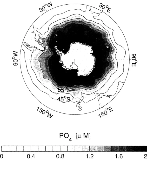
1-13 Annual mean surface phosphate distribution in the Southern Ocean based on the World Ocean Atlas 2001 (Conkright et al., 2002). Contour

interval is 0.4 ,t M. ... 46

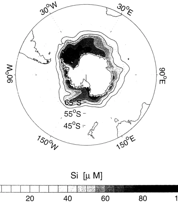
1-14 Annual mean surface silicic acid distribution in the Southern Ocean based on the World Ocean Atlas 2001 (Conkright et al., 2002). Contour

interval is 20 M. ... 47

(14)

1-15 Reconstructed export production for the LGM minus today (Bopp et al., 2003). This figure shows whether the export was higher at LGM (triangle), lower at LGM (square), or remained the same (cir-cle). The two solid lines are the mean latitudes of the Polar Front and

the Subantarctic front. . . . ... 52

2-1 (Left): The time history of anthropogenic CO2 between 1750 and 1950.

(Right) : The time history of CFC11, anthropogenic CO2 and

bomb-induced A14C between 1950 and 1990. The vertical axis is the

nor-malized atmospheric concentration. Atmospheric CO2 has the longest

anthropogenic perturbations ... 58

2-2 Geostrophic streamlines (a), and zonally averaged potential density field from Levitus climatology (b). The geostrophic streamlines are calculated from the 4 year time-averaged field of TOPEX-POSEIDON

data. The contour interval is 103_[m2s-1]. _{The potential density data}

is from Levitus climatology (Levitus 1994). ... 59

2-3 Observed pCFC11 distribution from WOCE (left column) in the lati-tude coordinate, and (right column) in the streamline coordinate. The units are in pptv, and the tracer data is obtained from WOCE line A-16 for (a,b), I-08 for (c,d) and P-15 for (e,f). The units for streamlines are 104m2s- 1 in (b,d,f). The two vertical lines in (b,d,f) marks the

position of the Polar Front and the Subantarctic Front. ... 60

2-4 Climatological surface wind stress plotted in (a) the longitude - latitude coordinate and (b) the longitude - streamline coordinate. The data is taken from long-time mean NCEP-NCAR reanalysis. The units are in

10-1N m- 2 ... 6 2

2-5 Climatological surface buoyancy plotted in (a) the longitude - latitude coordinate and (b) the longitude - streamline coordinate. The data is taken from long-time mean NCEP-NCAR reanalysis. The units are in

(15)

26 Climatological surface buoyancy flux plotted in (a) the longitude -latitude coordinate and (b) the longitude - streamline coordinate. The data is taken from long-time mean NCEP-NCAR reanalysis. The units

are in 10- 7 m2 s- a. ... 64

2-7 A schematic diagram showing the dynamical balance in the ACC. Eu-lerian mean flow and eddy-induced flow are shown as solid lines and dashed lines. They can be diagnosed from surface physical forcing

including wind stress and buoyancy fluxes. ... 68

2-8 Streamline averaged surface fluxes from NCEP-NCAR reanalysis data, the da Silva dataset, and the SOC dataset. (a): the buoyancy flux in units of m-2s- 3. (b): the surface wind stress in units of N m- 2. The horizontal axis is in streamline coordinate, and the two vertical lines

marks the position of the Polar Front and the Subantarctic front. . . 70

2-9 The residual stream function calculated using the idealized surface wind stress and buoyancy fluxes using the method of characteristics.

The units are in Sv ... 71

2-10 Simulated and observed distribution of CFC11 and its associating pCFC11. (a,b): the distribution of simulated CFC11 and pCFC11. (c,d): the distribution of observed CFC11 and pCFC11 from a WOCE Indian sec-tion, 1-08. The modeled fields are taken for the model year 1994 which

roughly corresponds to the periods of WOCE Indian section (I-08). . 73

2-11 Simulated and observed distribution of bomb-A14C. (a): the modeled

distribution. (b): the observed distribution along the WOCE Indian section (I-08). Bomb-Al4C distributions are separated from natural A1 4C using the potential alkalinity method of Key and Rubin (2002). 74

(16)

2-12 Scatter diagram of CFC11 and bomb-Al4C in the Southern Ocean to the south of 45S. (a): The diagram is based on the WOCE line 1-08. (b): The diagram is based on modeled distributions from the tracer model. Solid lines are the least-square fit to the data. In the surface layer, CFC11 and bomb-Al4C distributions are negatively correlated. Below the surface layer, the correlation becomes positive. The model

captures the gross pattern of the correlation. ... 74

2-13 Schematic diagram of the uptake of CFC11. Large scale upwelling drives strong uptake of CFC11 to the south of the ACC and isopycnal stirring drives another peak the uptake in the north of the ACC. In between, there is a region of minimum uptake due to the equatorward

advection and heating of surface waters. ... 76

2-14 Schematic diagram of the uptake of bomb-A14C. The gas transfer

coefficient controls the uptake. The maximum uptake occurs where the surface wind is at a maximum. In contrast the surface distribution

of bomb-Al4C reflects the large scale circulation. The surface gradient

in the concentration of bomb-A14C is due to equatorward residual flow. 76

2-15 Scatter diagram of CFC11 and bomb-Al4C in the Southern Ocean to the south of 45S calculated in the MITgcm. The diagram is based on the simulated distribution at the location of the WOCE line 1-08. The model does not reproduce the observed pattern of the correlation in

the surface layer. ... 78

2-16 Simulated meridional overturning circulation diagnosed from the OCMIP

run of MITgcm. The residual mean circulation, ,,es, plotted here is

based on the annual mean, net transport including Eulerian mean flow

and eddy-induced circulation parameterized using GM90. ... 79

2-17 The CFC11-bomb A14C scatter diagram from a subset of sensitivity

experiments with the zonally averaged model. Three cases are pre-sented here for ,,,e = 0, 10 and 15 Sv. The slope of the surface trend,

(17)

2-18 Simulated meridional overturning circulation diagnosed from the sen-sitivity calculation using MITgcm (MIT-O1). The residual mean circu-lation, ,,res, plotted here is based on the annual mean, net transport including Eulerian mean flow and eddy-induced circulation

parameter-ized using GM90. The contour interval is 5 Sv. ... 84

2-19 Simulated meridional overturning circulation diagnosed from the sen-sitivity calculation using MITgcm (MIT-02). The residual mean circu-lation, tres, plotted here is based on the annual mean, net transport including Eulerian mean flow and eddy-induced circulation

parameter-ized using GM90. The contour interval is 5 Sv. ... 85

2-20 Scatter diagram of CFC11 and bomb-Al4C in the Southern Ocean to the south of 45S calculated in the MITgcm (MIT-01). The diagram is based on the simulated distribution in the Atlantic (30W), Indian (90E) and Pacific 150(E) sections. The dashed line represents the

zonally-averaged tracer distributions. ... 86

2-21 Scatter diagram of CFC11 and bomb-A14C in the Southern Ocean to

the south of 45S calculated in the MITgcm (MIT-02). The diagram is based on the simulated distribution in the Atlantic (30W), Indian (90E) and Pacific 150(E) sections. The dashed line represents the

zonally-averaged tracer distributions. ... 87

2-22 Synthesis of the results from the simple 2D model, GCMs and

observa-tions (WOCE). The vertical axis is the slope of the CFC11-bomb A14C

diagram for the surface ocean in units of per mil pM-l. Dashed lines represent results from the 2D model. The gray region is the value in-ferred from observation. The two circles represent the value calculated

from the two GCM experiments. ... 88

(18)

2-23 Cumulative uptake of CFC11. Three panels are for the sensitivities to

Tres (a), · (b), and Kw (c). For control runs we use a standard set

of physical parameters. For sensitivity runs, we modified the physical parameters by multiplying a constant to the profiles of buoyancy fluxes,

wind stress, or gas transfer coefficient. Control simulation uses Tres=

14(Sv) and I = 32(Sv). ... 92

2-24 Cumulative uptake of bomb-Al4C between 1950 and 1990. Three pan-els are for the sensitivities to ,Tre (a), I (b) and Kw (c). The uptake has units of [permil m], and is plotted as a function of mean latitude.

Solid lines represent the control run. ... 97

2-25 Modeled and observationally-derived fields of anthropogenic CO2. (a):

the simulated distribution using the 2D model. (b): the observationally-derived distribution calculated by Sabine et al. (1999). The observa-tional data is obtained from Global Ocean Data Analysis Project, and

the plot (b) is reproduced with a permission. ... 99

2-26 Cumulative uptake of anthropogenic CO2 between 1765 and 1990.

Three panels are for the sensitivities to ,,re (a), i (b) and Kw (c). The unit of CO2 flux is in [mol/m2], and is plotted as a function of

mean latitude. Solid lines represent the control run. ... 100

3-1 Annually averaged organic export. The data is derived from an inverse calculation fitting modeled, large-scale tracer distribution to climatol-ogy. The data is taken from Schlitzer (2000). Organic export is in

units of gC m- 2 _{yr- .} _{. . . .} _{. ...} ₁₁₁

3-2 Observed sinking particulate flux of organic carbon and biogenic silica

at the depth of 1000m. The data is based on the mooring deployed

in the Pacific sector of the ACC during 1996 and 1998 (Honjo et al.,

(19)

3-3 Optimal solutions for the export of biogenic silica evaluated at the depth of 100 m. Three solutions are presented with varying magnitudes of a. A priori estimates of silica export is calculated from the data provided by (Honjo et al., 2000). The magnitude of error bars are adjusted to prohibit negative solution since each element of p must be

positive. ... 120

3-4 Optimal solutions for the distribution of the silicic acid. Three solu-tions are presented with varying magnitudes of a. Vector plot repre-sents the residual mean circulation which are used in the tracer

trans-port model. . . . ... .. .... 121

3-5 Variation of the magnitude of the two components of the cost function

with varying a. ... 122

3-6 Comparison of the two tracer tendency terms; advective tendency, -J(Q,,r, Si), and diffusive tendency, VKVSi. In this particular case, ac is set to 1. The net effect of physical transport is the sum of these two terms and it balances the uptake of silica in the surface layer of

the model. . . . ... 124

3-7 Distribution of the modeled silicic acid from the first 4 iteration cycles of the optimization using the adjoint method. The vector plots repre-sent the residual mean circulation. The system reaches very close to

the the optimal solution after a few iterations. ... 129

3-8 The profile of the silica export of biogenic silica from the first 4 iteration cycles of the optimization using the adjoint method. The initial guess is set to p = 0. The analytic solution is taken from the case with a =

0 ... 130

3-9 Comparison of two optimal solutions. In the control case, the silica export is calculated with the active residual mean circulation in the transport model. The solution is iteratively calculated through the adjoint method initialized with zero silica export. In the "'res = 0" case, the silica export is calculated by setting v,,res and wres to zero. . 132

(20)

3-10 Eulerian mean vertical velocity evaluated at the depth of 225m. ... 3-11 Parameterized, eddy-induced vertical velocity evaluated at the depth

of 225m. . . . ... 136

3-12 Residual mean vertical velocity evaluated at the depth of 225m. ... . 137

3-13 Simulated, annual-mean distribution of export production of organic

material. The Dash line represents Fe*(PO4) = 0 contour, marking

the position of the Antarctic Circumpolar Productivity Belt. ... . 141

3-14 Simulated, annual-mean distribution of export production of biogenic silica. The Dash line represents Fe*(Si) = 0 contour, marking the

position of the Antarctic Circumpolar Productivity Belt. ... 142

3-15 (Top) Simulated surface P0 4, Si, Fe distributions in a meridional

sec-tion in the Atlantic. (Bottom) Simulated profile of export producsec-tion in a meridional section in the Atlantic. The magnitudes of the con-centrations are scaled such that all nutrients become comparable. The scaling factors are set to the uptake ratios of the nutrients specified in

the model. . . . ... 144

3-16 Simulated Fe* distribution in (a) the global ocean and (b) the Southern Ocean. The dashed line in (b) and (c) represents the regime transition between iron-limited Antarctic zone and the macro-nutrient limited Subantarctic zone. The simulated productivity belt (c) is close to the

regime transition. . . . ... 146

3-17 Simulated Fe* distribution in (a) the global ocean and (b) the Southern Ocean. The dashed line in (b) and (c) represents the regime transition between iron-limited Antarctic zone and the macro-nutrient limited Subantarctic zone. The simulated productivity belt (c) is close to the

regime transition. . . . ... 147

3-18 Schematic diagram showing the mechanisms controlling the position of

the productivity belt ... 148

(21)

4-1 The observed pattern of changes in biological productivity between glacial and inter-glacial conditions can be accounted for by a northward shift of the productivity belt during ice ages. The position of the Polar Front in modern conditions is close to the node of the dipole pattern

in the paleo-productivity proxies. ... 153

4-2 Schematic diagram showing the response of the surface nutrient distri-bution and the position of the productivity belt in the Southern Ocean. The arrows point to the position of the transition between iron-limited

and macro-nutrient limited regimes. ... 156

4-3 Schematic diagram showing the two-cell structure of the meridional

overturning circulation in the Southern Ocean. Jires, changes its sign

between the two cells: ,,re is positive in the upper cell, and negative

in the lower cell. ... 159

4-4 Observed silicic acid distribution in WOCE section, A-16. ... 160

4-5 Sensitivity of the surface residual mean flow to the surface wind stress. 163 4-6 Schematic diagram of the model architecture. The model has an

ide-alized bottom topography below the depth of -he, and the effect of the topography on the circulation is parameterized as a zonal pressure

gradient in the zonally-averaged momentum equation. ... 168

4-7 The northern boundary condition, g(z), with varying z*. ... 171

4-8 Sensitivity of ym to variation in 7r. 7r0 represents the value for the control run, 7r0 = 10- 3. (a) The solution for ym as a function of 7r. (b) The position of the cell partition for three cases: the case with a 30%

reduction in r, the control run, and the case with a 30% increase in 172

4-9 Sensitivity of Ym to variation in z*. (a) The solution for Ym as a function of z*. (b) The position of the cell partition for three cases: the case with a 30% reduction in z*, the control run, and the case with a 30%

increase in z* ... ... 173

(22)

4-10 A schematic diagram for the response of the cell partition to rl and z*. The contour represents relative displacement of the position of the cell

partition ... ... 177

4-11 A schematic diagram for the response of the cell partition to rl and z* 181

5-1 Distribution of Preg, regenerated phosphate based on the WOCE-JGOFS survey. (a) WOCE line A-17 and A-20 in the Atlantic Ocean, (b) WOCE line P-18 in the Pacific Ocean. We use in-situ oxygen and hy-drographic data to calculate AOU. Observed data is interpolated on to a latitude-depth grid whose horizontal resolution is 1 and vertical resolution is 100 m. While general patterns of AOU clearly indicate the integrated effect of respiration, one has to be cautious about its inter-pretation. Significant undersaturation of oxygen and other trace gases is observed in the ice-covered surface polar oceans (Weiss et al., 1979; Schlosser et al., 1991), suggesting that preformed oxygen concentration may be lower than saturation particularly in the cold deep waters. If preformed oxygen concentration is undersaturated, AOU overestimates

the effect of respiration and so does the regenerated phosphate. . . . 192

5-2 Preformed phosphate distribution based on WOCE-JGOFS survey. Data is taken from (a) line A-17 and A-20, (b) line P-18. Waters formed in the Southern Ocean have approximately 1.6 puM of preformed phos-phate based on the calculation using AOU (5.2) which may include a

bias due to the oxygen disequilibrium. (See caption for Fig.1) .... 193

5-3 A schematic diagram for the major pathways of macro-nutrients in the oceans. The upwelling of nutrient is balanced by (1) biological uptake and export and by (2) subduction and formation of water masses. Here

(23)

5-4 A schematic diagram of the idealized atmosphere-ocean carbon cycle model. The model is configured for a rectangular basin with an open channel in the southern hemisphere. Periodic boundary conditions are used for the latitudes between 40S and 60S from surface to 2000m

depth ... 204

5-5 Steady state physical circulation. (a) Barotropic stream function is the depth integrated flow. Contour spacing is 10 Sv (b) Meridional over-turning circulation is the zonally averaged overover-turning circulations. Contour spacing is 2 Sv. Top, middle and bottom panel represent Eu-lerian mean flow, eddy-induced flow and the "residual" (or "effective") flow. The residual circulation is the sum of the Eulerian mean and the

eddy-induced circulation. . . . ... 205

5-6 Modeled phosphate, oxygen and DIC in the control run. (a) Zonally averaged phosphate at steady state. Contour interval is 0.4 IL M. (b) Zonally averaged oxygen at steady state. Contour interval is 50 ,/ M. (c) Zonally averaged DIC distribution at steady state. Contour interval

is 50 M. ... 208

5-7 Zonally averaged carbon pump components at steady state in the con-trol run. (a) Preformed phosphate, Pp,, in units of AM. Contour

interval of 0.4 M. (b) Regenerated phosphate, Preg, with the same

units and contour interval as (a). (c) Saturated carbon component, Csat, in units of IM. Contour interval is 50 /LM. (d) Disequilibrium

component, AC, in units of uM. Contour interval is 10 M ... . 209

5-8 Simulated response of atmospheric CO2, global mean Pp, and mean

surface P to the variation of the biological uptake timescale. ... 211

5-9 Simulated co-variation of atmospehric CO2 to the global mean Ppe . 212

5-10 Relationship between the global mean Ppr and the mean surface P . 214

5-11 Preformed phosphate at a high latitude surface outcrop is elevated due

to the vertical supply of phosphate through convective mixing .... 215

(24)

5-12 Carbon inventory difference relative to the control run. We consider the

partition of carbon among four reservoir; (1) atmosphere, MpCOat_m,

(2) saturated component, V Csat, (3) regenerated component, V Crg

(25)

List of Tables

2.1 Simple formulae for saturated concentrations of CFC11, anthropogenic

CO2 and bomb-A14C. kCFCll is the solubility of CFC11. DIC and

PCO20 are preindustrial distribution of DIC and pCO2 in the surface

ocean. Bu is the Buffer factor. Detailed derivations are presented in

appendix ... 67

2.2 Air-sea gas exchange timescales following Broecker and Peng (1974). Kw is the gas transfer coefficient, and B, is the Buffer factor. ko 2

is the solubility of C02. See appendix for detailed definitions of these parameters. We parameterize the gas transfer coefficient, Kw, follow-ing Wanninkhof (1992) with idealized profiles of temperature, salinity,

and surface wind. ... 67

2.3 Comparison of the numerical models. TRE89 represents the monthly climatology of (Trenberth et al., 1989). BF, HF and FH represent buoyancy flux, heat flux and fresh water flux respectively. V97 and GM90 represent the eddy parameterization of (Visbeck et al., 1997) and (Gent and McWilliams, 1990). Ar and Kv represent the isopycnal

eddy diffusivity and the vertical turbulent diffusivity. ... 81

2.4 Summary of the sensitivity experiments. std(A) represents the stan-dard deviation of A. For the simple 2D model, std(A) is based on the inverse of the eigenvalues of the Hessian matrix. For GCMs, std(A) is based on the standard deviation of A from 128 meridional sections

simulated in the model. ... 89

(26)

4.1 Some paleo-proxies for physical and biogeochemical changes in the

Southern Ocean during the LGM ... 184

5.1 Constants used in the theory . . . .. .. 202

(27)

Chapter 1 Introduction

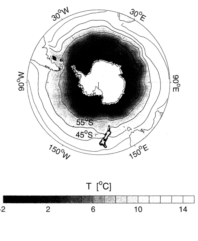
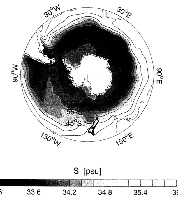
The Southern Ocean extends from the coast of Antarctica north to the southern part of the Atlantic Ocean, Indian Ocean and Pacific Ocean. The natural boundary between the northern basins and the Southern Ocean is the intense, eastward-flowing Antarctic Circumpolar Current (hereafter, ACC) and its associated quasi-zonal fronts where sharp changes in temperature, salinity and other properties are observed (Fig.l-1 and (Fig.l-1-2). The absence of topographic barriers in the latitude band of Drake Passage has important influences on the dynamics of the ACC and the transport of chemical and biological tracers there. A general review of the dynamics of the ACC can be found, for example, in (Rintoul et al., 2001). Here I briefly give an overview of some recent developments in understanding the dynamics and biogeochemistry of the Southern Ocean, which motivates several questions on the role of the Southern Ocean

in the uptake of anthropogenic CO2 into the oceans and past changes of the global

nutrient and carbon cycle.

Fig. 1-3 shows the horizontal pathway of the ACC calculated from the tempo-rally averaged geostrophic streamlines of the ACC based on the dynamic sea surface height, h. observed by the TOPEX-POSEIDON satellite altimeter. The currents rapidly circulate from west to east along the circumpolar streamlines. The mean pathway of the ACC is determined by the interplay between bottom topography and

1Geostrophic streamlines, g, are determined by T = h where g is the gravitational constant and f is the Coriolis parameter. In Fig.1-3 As varies by 5 .104 m2s- 1 across the Drake passage.

(28)

o 0 OD CO 0

m

T [C]

-2

2

6

10

14

Figure 1-1: Annual mean surface temperature distribution in the Southern Ocean based on -the World Ocean Atlas 2001 (Conkright et al., 2002). Contour interval is 4 C.

(29)

0 O' 03 (.O 0 m

S [psu]

11111111~ C ~ 71, I- -- I

33

33.6

34.2

34.8

35.4

36

Figure 1-2: Annual mean surface salinity distribution in the Southern Ocean based on the World Ocean Atlas 2001 (Conkright et al., 2002). Contour interval is 0.4 psu.

(30)

the conservation of potential vorticity (Gille, 1995; Marshall, 1995). This horizon-tal circulation connects the Atlantic, Indian and Pacific basins. While this quasi-horizontal, circumpolar current is the dominant feature of the ACC, the circulations in the latitude-depth plane are crucial to the transport of chemical and biological tracers. Fig.1-4 and 1-5 show meridional sections of neutral density and oxygen in the Atlantic and Pacific sector. Early researchers have interpreted the qualitative pattern of the meridional overturning circulation following the distribution of tracers such as temperature, salinity and oxygen (Sverdrup et al., 1942) (Fig.1-6). To the south of the ACC deep waters upwell into the surface layers, and near the Antarctic convergence (Polar Front), surface waters subduct into the ocean interior and form Antarctic Intermediate Water (AAIW).

1.1 Residual mean circulation

Recent theoretical and modeling studies have led to a better understanding in the mechanisms controlling the structure and rates of the meridional overturning circu-lation in the Southern Ocean. In the latitude band of the ACC, the net meridional geostrophic flow must vanish since the zonal pressure gradient integrates out to zero around the latitudinal circle. Thus the meridional transport of heat, salt and chemi-cal tracers must be carried by eddies below the base of the surface Ekman layer. In the surface Ekman layer, the interplay of the Ekman transport and the eddy-induced

transport determines the transport of tracers and air-sea fluxes of buoyancy, CO2,

CFCs and other trace gases (Marshall, 1997; Speer et al., 2000; Marshall and Radko, 2003; Ito et al., 2004). Thus the mesoscale eddy fluxes are fundamentally important for the biogeochemistry of the Southern Ocean. However, biogeochemical studies in this area typically use highly idealized, diffusive parameterization of mesoscale eddy fluxes. The goal of this thesis is to bring together recent views of ocean dynamics and biogeochemistry to examine and explore the role of the Southern Ocean in the global carbon cycle in the past and present.

(31)

circu-o

0)

-0

0

m

Figure 1-3: Geostrophic Streamlines of the ACC based on 4 year time-averaged

TOPEX-POSEIDON dynamic sea surface topography. Contour interval is 1 · 104

m2 sl. Data is provided by Center of Space Research, University of Texas, Austin.

(32)

350 C a 300 250 200 150 100 50 0 fX ons 50 'S4'S ,a$s 2'S 10'S

xoX11

-S-;s L eo w afa r o, ate

Figure 1-4: Meridional section of neutral density (contour) and oxygen (gray scale) in the Atlantic section. The data is taken from the WOCE hydrographic and bottle data (A-16) and plotted using Ocean Data View. The contour interval for neutral density is 0.5 for solid lines, and is 0.1 for dashed lines. The distribution of oxygen is generally oriented along isopycnals in the Southern Ocean. The newly ventilated Subantarctic

Mode Water (SAMW: 26.5 < < 27.0) and the Antarctic Intermediate Water

(AAIW: 27.0 < y, < 27.5) are well oxygenated and spread into the northern basins. North Atlantic Deep Water (NADW: 28.0 < yn < 28.2) is relatively well oxygenated, and is entrained and mixed with Circumpolar Deep Waters as it enters into the Southern Ocean. The Upper Circumpolar Deep Water (UCDW: 27.5 < %y < 28.0) and the Lower Circumpolar Deep Water (LCDW: 28.0 < y, < 28.2) are generally oxygen-depleted reflecting the influences of old, deep waters from the Pacific basin.

The Antarctic Bottom Water (AABW: 28.2 < yn) is ventilated from the continental

(33)

Q

H

350 300 250 200 150 100 50 I O

U-4S 5US 40US ?O'S 3 20'S EQ

Figure 1-5: Meridional section of neutral density (contour) and oxygen (gray scale) in the Pacific section. The data is taken from the WOCE hydrographic and bottle data (P-15) and plotted using Ocean Data View. The contour interval for neutral density is 0.5 for solid lines, and is 0.1 for dashed lines. The major difference between the Atlantic and Pacific sector is the difference in the influences of the northern basins. Deep waters in the North Atlantic are relatively new and well oxygenated, in contrast to the old, oxygen-depleted deep Pacific waters.

(34)

, . ... _ . -. a

A.

... t C, . - ANT

IG. . K"Xi\~'L

Figure 1-6: A schematic diagram of the meridional overturning circulation reproduced from (Sverdrup et al., 1942). The early researchers inferred the qualitative pattern of the circulation from chemical tracers.

(35)

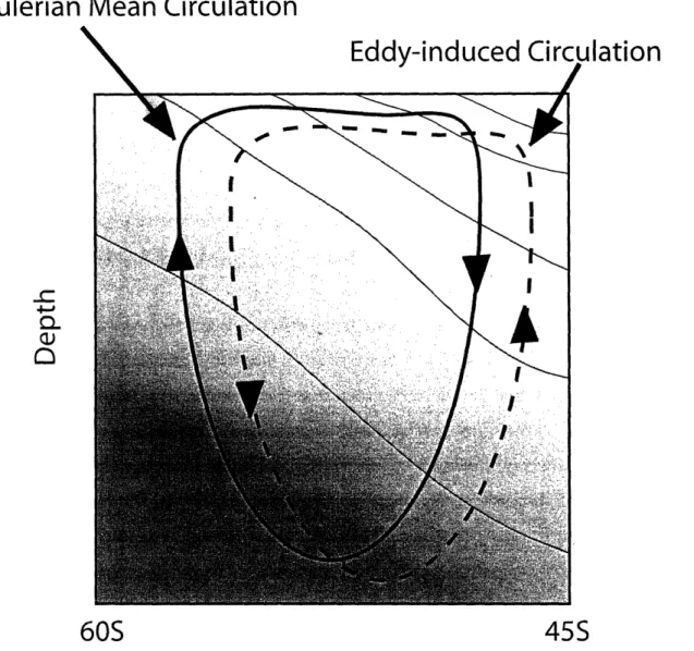
lation in the ACC. The westerly wind drives an equatorward Ekman circulation in the surface layers. The Eulerian mean, meridional overturning circulation, widely known as the Deacon cell, is driven by the surface Ekman transport and geostrophic return flow in the interior ocean supported by the deep topography. The wind-driven upwelling of relatively cold deep waters and downwelling of relatively warm surface waters tend to tilt isopycnals producing the available potential energy of the mean flow. The effect of baroclinic eddies is to extract the potential energy and flatten the

isopycnals, which results in the eddy-induced, meridional overturning circulation2_,

partially canceling out the wind-driven Eulerian mean circulation (Johnson and Bry-den, 1989). Temperature, salinity and other tracers are advected by the residual mean flow, the net effect of the Eulerian mean and the eddy-induced circulation.

Furthermore, there is a thermodynamic constraint that density must be conserved following the residual mean circulation since the diabatic component of eddy fluxes and diapycnal mixing are relatively small away from surface and bottom boundary layers (Marshall, 1997; Speer et al., 2000; Karsten et al., 2002), consistent with the observed distribution of chemical tracers which can be seen to spread along the isopy-cnal surfaces. Chemical tracers integrate (over time) the effects of a relatively weak, meridional overturning circulation. The distributions of long-lived tracers reflect the pattern of residual mean flow, which gives some sense of overturning circulation shown in Fig. 1-4, 1-5 and 1-6. The transport of carbon and nutrients by the residual mean circulation are the key factors in controlling biological productivity, global carbon

pumps, and the uptake of anthropogenic CO2 in the region. In this thesis, I

for-mulate simple models of physical-biogeochemical coupling in the framework of the residual mean theory.

2

See, for example, (Gill, 1982) for a general review of baroclinic instability theories and the eddy-mean flow interactions.

(36)

Eulerian Mean

Circulation

Eddy-induced Circulation

I

z100 ." .ft

I.

I cJ Q. D7

60S

45S

Figure 1-7: A simplified view of the meridional overturning circulation in the Southern Ocean

(37)

1.2 The uptake of anthropogenic CO

2

The oceans are the largest sink of fossil fuel CO₂ in the ocean-atmosphere-land

sys-tem, and recent research indicates that the Southern Ocean is one of the major regions

of CO2 uptake. 7.1 ± 1.1 PgC (1 PgC = 1015 gC) of carbon was emitted annually

into the atmosphere during the 1980s due to human activities, and the emission rate continues to rise. Recent studies suggest 2.0 ± 0.8 PgC were taken up annually into the global oceans during 1980s (Siegenthaler and Sarmiento, 1993; Takahashi

et al., 2002). However, the rate at which the oceans absorb anthropogenic CO2 and

its spatial distribution are difficult to determine from direct observations because the anthropogenic perturbations are small compared to the background,

naturally-occurring CO2fluxes. Furthermore ship-based observations are sparse in time and

space. For this reason ocean general circulation and biogeochemical model simula-tions have been used to provide additional estimates of the distribution and fluxes of

anthropogenic CO2. The Ocean Carbon-cycle Model Inter-comparison Project

(here-after, OCMIP) examined and compared several general circulation model (here(here-after, GCM) simulations of anthropogenic tracers(Orr et al., 2001; Dutay et al., 2002). Orr et al. (2001) suggest that the Southern Ocean is a major region of ocean uptake of

anthropogenic CO2 in the models, but also find that it is the region where the models

show the largest disagreement in the air-sea CO2flux. Fig.1-8 shows simulated,

zon-ally averaged uptake of anthropogenic CO2 uptake into the global oceans from four

OCMIP-1 models. Due to the large surface area of the Southern Ocean, the total

CO2 uptake is the greatest there in most of the models. However, the differences

between the models are large, and understanding the processes which cause these

differences is crucial for improving current estimates of the CO2uptake by the oceans

and future climate change. These coarse resolution models typically have horizontal resolution of >100 km, and do not resolve mesoscale eddies whose length scale is on the order of 10 km. Thus the mesoscale eddy fluxes are parameterized. Some re-cent biogeochemistry models apply the isopycnal thickness diffusion scheme of (Gent and McWilliams, 1990) which includes the advective fluxes of eddies in the sub-grid

(38)

scale eddy parameterization, and those models better reproduce the distribution of transient tracers such as CFCs in the Southern Ocean (Robitaille and Weaver, 1995).

The air-sea CO2 flux is driven by the disequilibrium between the partial pressure

of CO2 in the atmosphere and the sea surface, which is maintained by the interplay

between physical circulation, chemical and biological processes. The timescales of air-sea CO2 equilibration is on the order of a year (Broecker, 1974), suggesting that

the air-sea gas exchange is unlikely to be the rate limiting process in the uptake of

CO2 into the surface oceans. Surface waters will reach saturation with atmospheric

CO₂ within a few years if the surface layer is stagnant and does not interact with interior ocean. The renewal of surface waters by the upwelling and entrainment of thermocline waters is required to maintain the surface undersaturation and uptake of

anthropogenic CO2 into the surface oceans. Therefore, the pattern and the

magni-tude of the residual mean flow can play the central role in determining the uptake of

anthropogenic CO2 through controlling the rate of upwelling and renewal of the

sur-face waters in the Southern Ocean. Mesoscale eddy fluxes and the parameterization of them might be the key process limiting our ability to predict the regional uptake of CO2.

In chapter 2, I develop zonally averaged model of tracer transport in the ACC based on the residual mean theory, and use the model to estimate the uptake of

transient tracers including CFCs, bomb radiocarbon, and anthropogenic CO2. The

simplicity of the model allows us to illustrate the relative roles of lateral advection, entrainment of thermocline waters and isopycnal stirring of tracers in controlling the tracer uptake and its regional variation. Scaling relationships are derived for the sensitivity of tracer uptake for each tracer. Tracer distributions are strongly influenced by the ocean circulation. In turn, observed tracer distributions can help constrain the rates of the meridional overturning circulation.

(39)

!

1.5

15

0.5 _ 0.04 IB 0.01 lAitide

Figure 1-8: Simulated profile of the anthropogenic CO2 uptake from the OCMIP-1

models. This figure is reproduced from (Orr et al., 2001). These early models do not include advective influences of eddies in their sub-grid scale eddy parameterization.

39

(40)

1.3 Biological pump of CO

2 during the Last Glacial

Maximum

The biogeochemistry and physical circulation of the Southern Ocean could have played

important roles in past climate changes. Atmospheric partial pressure of CO2over

the past 420,000 years is reconstructed from polar ice cores (Petit et al., 1999) and

re-vealed that the atmospheric pCO2and the polar atmospheric temperatures are tightly

coupled with one another. Fig. 1-9 shows the variation of atmospheric pCO2 and

po-lar atmospheric temperature derived from the Vostok ice core. At the Last Glacial Maximum (hereafter, LGM: approximately 12,000 years ago) polar temperatures were

cooler approximately by 10°C and atmospheric pCO2was lower than the preindustrial

condition approximately by 80 ppmv. A number of theories have been suggested to

explain the link between the glacial climate and the lowered atmospheric pCO2.

Some researchers argue that biological pump of C0 23 was more efficient during ice

ages due to the changes in the biogeochemistry and physical circulation of the South-ern Ocean. So-called the "Harvardton Bear" models, which were developed during 1980s by groups at Harvard, Princeton and Bern universities (Sarmiento and Togg-weiler, 1984; Siegenthaler and Wenk, 1984; Knox and McElroy, 1984), have shown that a drawdown of sea-surface nutrients in the high latitudes is sufficient to cause

a decrease in the atmospheric pCO2 comparable to those recorded in ice cores. A

schematic diagram (Fig. 1-10) illustrates how high-latitude surface nutrients may be

related to atmospheric pCO2. The model consists of low-latitude and high-latitude

surface oceans, and a deep ocean. At low latitudes, surface nutrients are almost com-pletely utilized, and the export of organic material vertically transfers nutrients and carbon from the surface layer to the deep layer. Due to the density structure of the oceans, the deep waters are ventilated through the polar outcrop, and so chemical

3_{Photosynthesis in the surface ocean converts inorganic carbon and nutrients into organic matter,}

often accompanied with calcium carbonate structural material. A fraction of the organic matter described as export production, is ultimately transported to, and remineralized within, thermocline and abyssal ocean. Vertical transfer of CO02 due to the export of organic material is termed as soft

tissue pump and that of calcium carbonate as carbonate (hard shell) pump. The biological pump of

(41)

pC02 -'T

280 ...

260. 220 I.. i

I...

...

nn

220

1 -I

\r

:

....

1 ...

n n

I

... . .

...

I

~I

I

...

· #:

I

,.--4

_,

_J

_{I --}

_{w 'r}

_A

-

_-

_'

_iV

2 i

.q

-8P,!i

i

I

..

.

: ··.·

~

:;··9-. .

· · · ·· · · · ·

.

.l i .... i.. I I :. I:

_..

'-'

0

50 100 150 200 250 300 350 400

Age kyrBP

Figure 1-9: Atmospheric pCO2 and polar atmospheric temperature reconstructed

from the Vostok ice cores (Petit et al., 1999). The horizontal axis is the "age" of ice in units of kyr BP (1,000 years before present). The progression of time is conventionally defined from right (old) to left (recent).

41

(42)

properties of high-latitude surface oceans and that of deep waters significantly

influ-ence one another4. The Southern Ocean is characterized with elevated macro-nutrient

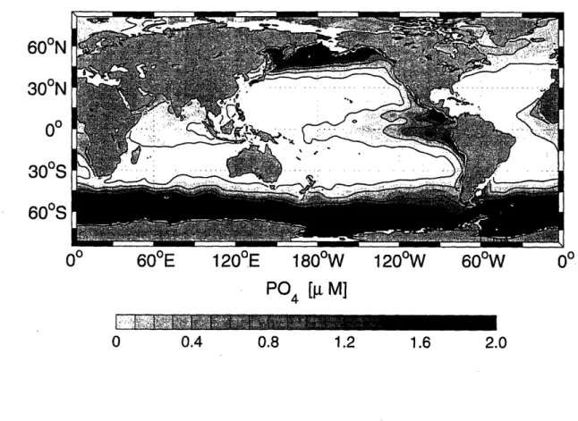
concentration in present climate (see Fig. 1-11). As the deep waters are entrained into

the surface waters, a fraction of CO2 sequestered by the biological pump at low

latitudes is released into the atmosphere. Elevated surface nutrient concentration indicates the inefficiency of the global biological pump. Surface nutrient concentra-tion is set by the competiconcentra-tion between the supply of nutrients by the upwelling and the removal by the biological uptake and export. When regional biological uptake is weak relative to the upwelling of nutrients, surface nutrient concentrations become

higher, and larger amount of CO₂ is transferred to the atmosphere by outgassing. In

the context of these highly idealized box models, there are two processes which can

decrease the surface nutrients and suppress the regional outgassing of CO2 at high

latitudes.

* Increased, regional biological uptake and export (Fig.1-10, case 1)

* Decreased upwelling of the deep waters to the surface layer (Fig.1-10, case 2) The first mechanism could have been supported by the supply of iron to the surface oceans through atmospheric dust deposition (Martin, 1990). Fig.1-11 and 1-12 show the annually-averaged, global distribution of macro-nutrients in the surface oceans. Fig.1-13 and 1-14 shows the distribution in the Southern Ocean. The concentration of phosphate and silicic acid is remarkably high in the polar Southern Ocean. The growth of phytoplankton is not limited by the supply of these macro-nutrients there. The biogeochemistry of the Southern Ocean has been considered as a "high nutrient low chlorophyll" (hereafter, HNLC) condition, where the rate of biological produc-tion, normalized by the available nutrient, is relatively low and surface macro-nutrients are not fully utilized. It has been suggested that the biological productivity in the HNLC region could be limited by the supply of micro-nutrients such as iron (Martin and Fitzwater, 1988). In-situ iron addition experiments in HNLC regions

4

Typically, the "preformed" properties of the deep waters refer to the properties of the polar outcrop at the time of the formation of water masses. As we discuss later in chapter 5, "preformed" nutrients play the central role in the theory of biological pumps.

(43)

Modern :high pCO2, high PH

low lat.

high lat.

LGM: low pCO2, low PH

Case (1)

_{Case (2)}

i

stronger export

at high latitudes

weaker upwelling

Figure 1-10: Schematic diagrams illustrating the influences of high latitude surface ocean in controlling the efficiency of the biological pump in the global oceans. PH represents high-latitude surface nutrient concentration. Arrows with dash line repre-sent fluxes of DIC due to chemical and biological processes including biological export and air-sea CO2 flux. Arrows with solid line represent fluxes of DIC due to physical

circulation. 43

I - l

M

t

I I

(44)

60°N

30°N

00

30

0

S

60

0

S

60

0

_E

₁₂₀

0

_E

₁₈₀

0

_W

_120°W

_60°W

PO

4

[ M]

o 0.4 0.8 1.2 1.6 2.0

Figure 1-11: Annual mean surface phosphate distribution in the global ocean based on the World Ocean Atlas 2001 (Conkright et al., 2002). Contour interval is 0.4 M.

(45)

60°N

30°N

00

30

0

S

60°S

0

°

₆₀

0

_E

₁₂₀

0

_E

₁₈₀

0

_W

₁₂₀

0

_W

₆₀

0

_W

₀

°

Si [ M]

0 20 40 60 80 100

Figure 1-12: Annual mean surface silicic acid distribution in the global ocean based

on the World Ocean Atlas 2001 (Conkright et al., 2002). Contour interval is 20 M.

(46)

0 0 (O 0

PO

4 [ M]

I I

1

0 I

I I

I1.6

1.2

2.0

0

0.4

0.8

1.2

1.6

2.0

Figure 1-13: Annual mean surface phosphate distribution in the Southern Ocean based on the World Ocean Atlas 2001 (Conkright et al., 2002). Contour interval is

(47)

C

a)

.0 o 0

m

Si [

M]

[1

I '

I

. I ""···*,

0

20

40

60

80

100

Figure 1-14: Annual mean surface silicic acid distribution in the Southern Ocean based on the World Ocean Atlas 2001 (Conkright et al., 2002). Contour interval is

20 M.

(48)

revealed that primary production in these regions indeed responds to the addition of iron to the surface waters (Martin et al., 1994; Coale et al., 1996; Boyd et al., 2000) although its impact on the export of organic material out of euphotic layer remains unclear. Increased atmospheric dust deposition during ice ages could have increased local biological productivity, leading to a drawdown of surface nutrients and

atmospheric pCO2 (Martin, 1990).

Since 1990s it has become feasible to combine three-dimensional ocean general circulation models and parameterizations of nutrient and carbon cycles, allowing ex-plorations of the response of carbon cycle to increased rates of nutrient uptake in the surface ocean, mimicking elevated biological export (Sarmiento and Orr, 1991; Archer et al., 2000). These so-called "nutrient depletion" experiments help us to understand the response of carbon cycle to increased utilization of surface nutrients in the context of more realistic, three-dimensional ocean circulation. They find that

the sensitivity of atmospheric pCO2 to the depletion of polar surface nutrients is

sensitive to the profile of remineralization in the interior ocean (Sarmiento and Orr,

1991). Moreover, atmospheric pCO2 is less sensitive to a drawdown of high-latitude

surface nutrients in three-dimensional models than in box models, and the drawdown of polar nutrients cannot reproduce the glacial pCO2 (Archer et al., 2000). It is not

yet well understood what ultimately determines the sensitivity of atmospheric pCO2

to a depletion of polar surface macro-nutrients.

Furthermore, recent development of physical-biogeochemical model has introduced the coupling between ocean carbon cycle and the explicit iron cycle with ecosystem dynamics (Bopp et al., 2003; Parekh et al., 2004a). These models can qualitatively reproduce observed distribution of nutrients in the global oceans. Using these models, the biological productivity and carbon cycle are simulated with elevated atmospheric

dust deposition. However, the response of atmospheric pCO2 to an elevated aeolian

dust deposition is significantly smaller than the glacial-interglacial variations of pCO2

observed in ice cores. Therefore, it seems unlikely that the increased atmospheric dust

deposition can be the direct cause of - 100 ppmv drawdown of atmospheric pCO₂

(49)

The second mechanism involves changes in the the ventilation of the Southern Ocean. Recent research (Francois et al., 1997; Sigman and Boyle, 2000; Gildor and Tziperman, 2001) suggest that the vertical supply of nutrients significantly decreased during ice ages. They argue that the reduced upwelling of deep waters is caused by the stronger stratification and an equatorward shift of the westerly wind belt. Increasing the stability of water column may suppress convective mixing and decrease the supply of nutrients to the surface layer. Northward migration of the westerly wind belt might weaken the wind stress over the Southern Ocean. Surface wind stress drives near-surface Ekman transport, and to the south of the westerly wind stress maximum, the Ekman transport is divergent and deep waters upwell into the surface layer. Decreasing the surface wind stress weakens the Ekman upwelling and the vertical supply of nutrients. If the supply of nutrient is reduced and the biological productivity

is sustained, surface nutrients must be strongly depleted, and the outgassing of CO2

becomes weaker, leading to a lower atmospheric pCO₂

.

The wind-driven Ekman transport partially drives the meridional overturning cir-culation, however recent research highlights the significant role of mesoscale eddy fluxes leading to the "residual mean" view of the meridional overturning circulation. The representation of physical transport is highly idealized in previous studies of the

carbon cycle in the Southern Ocean. In particular, they do not consider the advec-tive influence of mesoscale eddies in the vertical supply of nutrients. The hypothesis of "polar stratification" is challenged by Keeling and Visbeck (2001) that increasing stratification in the Southern Ocean increases the rate of upwelling if the advective influence of mesoscale eddies are included. Theories of baroclinic instability suggest that eddy transports scale with the degree of baroclinicity, which is measured by the slope and the spacing of isopycnal surfaces (Gill, 1982; Pedlosky, 1986; Visbeck et al., 1997). Increasing the stratification decreases the baroclinicity of the region, leading to a weaker eddy-induced transport. Since the Ekman transport is partially compensated by the eddy-induced transport, weakening of the eddy fluxes leads to more pronounced Ekman transport.

Somewhat related to the "polar stratification" hypothesis is the extended sea ice 49

The biogeochemistry and residual mean circulation of the southern ocean

The biogeochemistry and residual mean

circulation of the Southern Ocean

by

Takamitsu Ito

Submitted to the Department of Earth Atmospheric and Planetary

Sciences

in partial fulfillment of the requirements for the degree of

Doctor of Philosophy

at the

MASSACHUSETTS INSTITUTE OF TECHNOLOGY

Feburary 2005

( Massachusetts Institute of Technology 2005. All rights reserved.

A uthor ...

...

...

Depart

nt of Earth Atmospheric and Planetary Sciences

'~~~~~1

7, 2004

Certified by..

John C. Marshall

Professor

Thesis Supervisor

Accepted by ...

Maria Zuber

Department Head, Department of Earth, Atmospheric and Planetary

Sciences

ARCHIVES

APR 14

25

I

.JI

LIBRARIES

'C/ .. k J

-The biogeochemistry and residual mean circulation of the

Southern Ocean

by

Takamitsu Ito

Abstract

Acknowledgments

Contents

List of Figures

List of Tables

Chapter 1

Introduction

m

T [C]

-2

2

6

10

14

S [psu]

33

33.6

34.2

34.8

35.4

36

1.1

Residual mean circulation

xoX11

H

Eulerian Mean

Circulation

Eddy-induced Circulation

I

I.

60S

45S

1.2

The uptake of anthropogenic CO

2

1.5

15

1.3

Biological pump of CO

2

during the Last Glacial

_,

_J

_{I --}

_{w 'r}

_A

_-

_'

_iV

_..

_{Case (2)}