HAL Id: hal-02343291
https://hal.archives-ouvertes.fr/hal-02343291
Submitted on 8 Nov 2019HAL is a multi-disciplinary open access
archive for the deposit and dissemination of sci-entific research documents, whether they are pub-lished or not. The documents may come from teaching and research institutions in France or abroad, or from public or private research centers.
L’archive ouverte pluridisciplinaire HAL, est destinée au dépôt et à la diffusion de documents scientifiques de niveau recherche, publiés ou non, émanant des établissements d’enseignement et de recherche français ou étrangers, des laboratoires publics ou privés.
A molecular-dynamics study of sliding liquid nanodrops:
Dynamic contact angles and the pearling transition
Juan-Carlos Fernández-Toledano, Terry Blake, Laurent Limat, Joël de
Coninck
To cite this version:
Juan-Carlos Fernández-Toledano, Terry Blake, Laurent Limat, Joël de Coninck. A molecular-dynamics study of sliding liquid nanodrops: Dynamic contact angles and the pearling transition. Journal of Colloid and Interface Science, Elsevier, 2019, 548, pp.66-76. �10.1016/j.jcis.2019.03.094�. �hal-02343291�
A Molecular-Dynamics Simulation of Sliding
Liquid Nanodrops
J-C. Fernández-Toledanoa*, T. D. Blakea, L. Limatb, and J. De Conincka
aLaboratory of Surface and Interfacial Physics (LPSI), University of Mons, 7000 Mons, Belgium bLaboratoire Matière et Systèmes Complexes, UMR 7057 of CNRS and University of Paris
Diderot, Sorbonne Paris Cité, France
Hypothesis: That the behavior of sliding drops at the nanoscale mirrors that seen in macroscopic
experiments, that the local microscopic contact angle is velocity dependent in a way that is
consistent with the molecular-kinetic theory (MKT), and that observations at this scale shed light
on the pearling transition seen with larger drops.
Methods: We use large-scale molecular dynamics (MD) to model a nanodrop of liquid sliding
across a solid surface under the influence of an external force. The simulations enable us to
extract the shape of the drop, details of flow within the drop and the local dynamic contact angle
at all points around its periphery.
Findings: Our results confirm the macroscopic observation that the dynamic contact angle at all
points around the drop is a function of the velocity of the contact line normal to itself, 𝑈!"sin𝜙, where 𝑈!" is the velocity of the drop’s center of mass and 𝜙 is the slope of the contact line with respect to the direction of travel. Flow within the drop agrees with that observed on the surface
of macroscopic drops. If slip between the first layer of liquid molecules and the solid surface is
accounted for, the velocity-dependence of the dynamic contact angle is identical with that found
previous MD simulations of spreading drops, and consistent with the MKT. If the external force
is increased beyond a certain point, the drop elongates and a neck appears between the front and
rear of the drop, which separate into two distinct zones. This appears to be the onset of the
pearling transition at the tip of a macroscopic drop. The receding contact angle at the tip of the
drop is far removed from its equilibrium value but non-zero and approaches a more-or-less
constant critical value as the transition progresses.
Keywords: Wetting, moving contact lines, avoided critical behavior, dynamic contact angle,
1. Introduction
Raindrops running or sliding down a windowpane are so much part of everyday experience
that one may rarely stop to consider the mechanisms that might determine their passage. Casual
inspection reveals that on a well-wetted surface, the drops move down nearly vertical paths. If
the window is initially dry, a drop may slide with an irregular trajectory, diverting first to one
side and then the other as its leading edge is hindered, generating unsteady internal flows. New
drops arriving on the same path may follow the track of their predecessor, or diverge, pioneering
their own trail. On a dry, but less easily wetted surface, the drops may stick and not start to
move until another drop arrives to increase their mass. Once sliding starts, the drop may take on
a teardrop shape, with a tapering, triangular tail from which even smaller drops are shed, as
illustrated in Figure 1a. Such shedding may seem unsurprising; is not the drag of the glass bound
to cause some fraction of the drop to be left behind? Nevertheless, this behavior is far from
Figure 1. a) Sketch of a sliding drop showing a trailing vertex and a detached drop. b)
Schematic of a saw-tooth wetting line formed when 𝑈 > 𝑈!"#$. c) Image of a triangular film entrained when a partially wetted surface is pulled vertically out of a bath of liquid [1].
A related phenomenon can be seen when a partially wetted plate or tape is pulled vertically out
of a pool of liquid. At sufficiently low speeds, the solid surface emerges from the pool in an
apparently dry state. However, if the speed of withdrawal exceeds a certain value, then a film of
liquid is entrained. As the plate is pulled upwards, the film, including its upper boundary (the
contact line) drains downwards, but at a slower rate, so that the wetted area increases. Of
particular interest is that the receding contact line does not usually remain horizontal, but
inclines, taking on a saw-tooth configuration. If the speed is increased still further, the film
lengthens and the vertex angle of each triangular section becomes increasingly acute.
Eventually, discrete drops of liquid are pulled from each trailing vertex.
Blake and Ruschak [1] showed that this behavior is evidence of a maximum velocity of
dewetting, 𝑈!"#$ beyond which a film will be pulled. In order to minimize the energetically unfavorable creation of a liquid film on a poorly wetted surface, the contact line lengthens to
form the saw-tooth shape, such that the normal velocity of each segment remains constant at its
maximum value. The general effect is quite predictable and, as illustrated in Figure 1b, there is a
simple geometric relationship between 𝑈!"#$, the withdrawal velocity of the plate 𝑈 and the angle of inclination 𝜙 of each segment with respect to the direction of motion:
𝑈!"#$ = 𝑈sin𝜙. (1)
In these experiments, a smooth, uniform 50 mm polymer tape was withdrawn continuously at
film was obtained across the width of the tape (Figure 1c). Drops were entrained from the
trailing vertex once 𝜙 was less than about 45º. At the vertex, where the two straight-line segments appear to intersect, the curvature of the contact line is large but finite; thus, the tangent
at this point will be horizontal and a local forced wetting transition leads to the entrainment of a
narrow rivulet of liquid by the solid. This subsequently breaks into individual droplets due to
Rayleigh-Plateau instability. The details of this region and exactly how the flow in the vicinity
of the contact line avoids this critical behavior along the inclined segments is not yet fully
explained, although progress has been made within certain simplifications, such as the use of the
lubrication approximation to describe the flow and a fixed local, microscopic angle [2–6]. The
situation is complicated by incomplete agreement on how a contact line moves across a solid
surface: in particular, the relative importance of viscous and surface frictional forces at the
contact line and whether or not it is indeed sufficient to assume that the microscopic contact
angle remains constant at its equilibrium value [7–11].
Since the pioneering work [1], there have been further experimental studies of both film
deposition [12–15] and sliding drops [3,16–20]. Recent papers [21,22] provide useful reviews,
as well as detailed theoretical analyses. Although the phenomenology of sliding drops has much
in common with film deposition, such as the avoided critical behavior and droplet shedding,
there are several potentially important differences, in particular their small size and the fact that
the liquid system is initially closed and surrounded by a highly curved surface. With respect to
flow near the trailing vertices and droplet shedding (the so-called ‘pearling transition’) good
agreement has been found between theory and experiment with moderately viscous silicone oils,
water [19]. Whether this is due to the three-dimensionality of the flow in this region, the
assumption of a fixed microscopic contact angle, or some other factor, remains to be resolved.
One approach that shows promise to further our understanding is to use large-scale molecular
dynamics (MD) to model droplet sliding. MD has proved uniquely successful in illuminating the
molecular mechanism by which a contact line moves across a solid surface and demonstrating
the importance of contact-line friction [23–37]. Indeed, a very recent paper by Lukyanov and
Pryer [38] may have successfully reconciled MD results with macroscopic hydrodynamics
yielding a regularized solution to the moving contact line problem. Here, we apply MD to model
a liquid nanodrop sliding across a molecularly flat solid surface under the influence of a uniform
force that acts parallel to the solid-liquid interface and is applied to all the atoms of the liquid;
thus, mimicking a drop sliding under the influence of gravity. We demonstrate that our results
are compatible with the physical experiments of Limat and co-workers [39] and extend our
understanding of the underlying processes down to the nanoscale.
2. Molecular dynamics
The simulation methods, base parameters and potentials we employ have all been used
previously by De Coninck and co-workers to successfully model a range of wetting problems
such as droplet spreading [27,34,35], the wetting of fibers [31], dewetting dynamics [32], and
forced wetting in Couette flow [36]. Full details are given in these publications and work cited
therein, where we have shown that the system, though very simple, has all the necessary features
to model wetting on the nanoscale and recover established macroscopic laws governing liquid
behavior. To summarize, the liquid (L), the solid (S) and their interactions are modelled using
𝑉 𝑟!" = 4𝜖𝐶!" !! !" !" − !! !" ! . (2)
Here, 𝑟!" is the distance between any pair of atoms 𝑖 and 𝑗. The parameters 𝜀 and 𝜎 are, respectively, the depth of the potential wells and an effective atomic diameter. For both solid
and liquid atoms, 𝜎 = 0.35 nm and 𝜀 = 𝑘!𝑇, where 𝑘! is the Boltzmann constant and 𝑇 = 33 K is the temperature. The pair potential is set to zero for 𝑟!" > 2.5𝜎. The coupling parameter 𝐶!" enables us to control the relative affinities between the different types of atoms and is given the
value 1.0 for both L-L and S-S interactions but varied for S-L interactions in order to explore the
influence of wettability on drop dynamics. Three values were selected: 𝐶!" = 0.7, 0.8, and 0.9, yielding equilibrium contact angles 90º, 75º, and 55º, respectively.
The solid plate, which forms the bottom of the simulation box, comprises 69048 atoms
arranged in a cubic lattice having three atomic layers with a lattice parameter 𝜆 = 2!/!𝜎 ≈ 0.393
nm, i.e., the equilibrium distance given by the Lennard-Jones potential. To maintain rigidity,
while permitting momentum exchange with the liquid, the solid atoms are allowed to vibrate
thermally around their initial positions by a strong harmonic potential:
𝑉! 𝑟 = 1000𝜖 𝒓 − 𝒓𝟎 ! 𝜎!, where r is the instantaneous position of a given solid atom and 𝒓𝟎
is its initial lattice position.
The liquid is modelled as 5000 8-atom molecular chains, with adjacent atoms linked by a
confining potential: 𝑉!"#$ = 𝜖 𝑟!" 𝜎 !. This increases its viscosity compared with a monomer liquid and minimizes evaporation within the timescale of the simulation, so that the vapor phase
is effectively a vacuum. The dimensions of the simulation box are 𝐿!, 𝐿!, 𝐿! = 107.6, 33.0, 30.0 nm, respectively, with periodic boundary conditions imposed in the 𝑥 and 𝑦 directions. To
investigate whether our results are independent of drop size, we also study a system comprising
10643 liquid molecules on a 3-layer cubic solid formed from 76608 atoms in a simulation box of
dimensions 𝐿!, 𝐿!, 𝐿! = 88.0, 44.7, 30.0 nm. The volumes of the smaller and larger liquid drops are (2.081 ± 0.003) × 103 nm3 and (4.201 ± 0.002) × 103 nm3, respectively, computed as the volumes of spheres fitted to the equilibrated surfaces of the drops before contact with the plate.
In order to compare our simulations with real, physical systems, all the atoms of both the
liquid and the solid are given the mass of the carbon atom (12 g/mol). The simulated liquid has a
density of 𝜌! = 18.26 ± 0.07 atoms/nm3, equivalent to 363.9 ± 1.4 kg/m3. Its surface tension is
𝛾!" = (2.49 ± 0.65) mN/m. This was found by an independent simulation of a free liquid film with planar surfaces from the integral of the difference between the normal and tangential
pressures through the interface [40]. We have also performed a simulation of the bulk liquid
with no interface to determine its viscosity 𝜂! = (0.249 ± 0.004) mPa·s from the diffusion coefficient 𝐷 via the Stokes-Einstein relation [41]. 𝐷 is measured from the slope of the mean square displacement of liquid atoms versus time [42] and has the value (0.562 ± 0.021) nm2/ns. Over the range of our simulations the liquid remains Newtonian: all its properties, including its
viscosity, are independent of the applied force and the velocity of the drop. Previous studies of
Couette flow have also confirmed this [36].
In the simulation, Newton's equations of motion are solved using a 5th order Taylor expansion
with a time step of 5 fs. The liquid molecules are initially distributed in a cubic lattice close to
the plate and the entire system equilibrated using a thermostat based on velocity scaling for 106
time steps (5 ns). During this period, the liquid atoms rearrange to form an equilibrium droplet,
achieved, the thermostat is applied to the solid atoms only (to mimic an isothermal solid, as in a
physical experiment) and we introduce an external force field in the x direction, parallel to the
S-L interface and acting on each liquid atom: 𝑭𝟎= 𝐹!𝒙, where 𝒙 is the unit vector in the 𝑥 direction and 𝐹! is given one of 8 values from 0.83 to 6.64 fN. This causes the liquid drop to translate across the solid surface at a velocity that depends on both the strength of the field and
the S-L coupling. The velocity attains a steady value well within the 5 × 10⁶ time steps (25 ns) allowed for this stage of the simulation. During this period, the drop also acquires constant
overall dimensions and shape. Finally, we continue the simulation for another 5 × 10⁶ time steps, saving the positions of the liquid atoms at intervals of 103 time steps. The resulting data enable
statistical analysis of the sliding drops over 5 × 10³ saved configurations.
Molecular-dynamics modelling has the advantage over experiment that all the material
properties and kinematic behaviors can be determined independently down to the molecular scale
under a very wide range of conditions. This includes the degree to which a liquid droplet wets
the solid and the way this may change when the droplet moves. In our simulations, wetting is
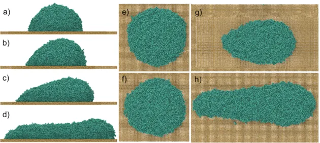
controlled by the solid-liquid coupling 𝐶!". Figure 2 illustrates instantaneous (unaveraged) snapshots of a simulated drop for 𝐶!" = 0.7, which yields an equilibrium contact angle 𝜃! of 90˚,
and various values of the force defined by 𝐹!. The forces and the resulting motions are from left
to right in the snapshots. The caption also gives the velocity of the drop’s center of mass 𝑈!"
and the equivalent capillary number Ca = 𝜂!𝑈!" 𝛾!". The drop shapes and their evolution closely resemble those seen in experiments [16– 20,39,43]. As the drops are very small, 𝐹! has to be orders of magnitude greater than that caused by gravity to overcome the very large
capillary forces generated as the drops slide and their configurations and contact angles change
sliding raindrops, however the equivalent capillary numbers are realistic and not significantly
larger than observed in experimental studies of forced wetting. We discuss these aspects of the
study in more detail below.
Figure 2. Instantaneous snapshots for 𝐶!" = 0.7. a) lateral and e) top view for 𝐹! = 0.83 fN, 𝑈!" = 2.7 m/s, Ca = 0.27. b) lateral and f) top view for 𝐹! = 1.66 fN, 𝑈!" = 4.86 m/s, Ca = 0.49. c) lateral and g) top view for 𝐹! = 3.32 fN, 𝑈!" = 9.9 m/s, Ca = 0.99. d) lateral and h) top view for 𝐹! = 4.98 fN, 𝑈!" = 11.1 m/s, Ca = 1.11.
3. Results and Discussion
3.1 Drop velocities and the shape of the contact line.
In order to analyze the dynamics of a sliding drop, we need to determine the location of the
three-phase contact line, corresponding to the intersection of the liquid-vacuum interface with
the solid surface. To compute this at all points around the drops, we refer the position vector of
each liquid atom 𝑖, 𝒓𝒊(𝑡) to the location of the drop mass center at time t, 𝒓𝒄𝒎(𝑡), i.e., 𝒓′𝒊 𝑡 = 𝒓𝒊 𝑡 − 𝒓𝒄𝒎(𝑡). The liquid-vacuum interface may then be defined as the surface over which the local liquid density 𝜌!(𝒓′𝒊, 𝑡) falls to half that of the bulk liquid (i.e., the equimolar surface). To
measure the density 𝜌! 𝒓!, 𝑡 , we subdivide the available volume of the drop into cubic cells of
size 𝑑𝑥, 𝑑𝑦, 𝑑𝑧 = 0.3 nm and calculate the average number of atoms per cell over 500 configurations at intervals of 103 time steps. More details are given in Supporting Information.
At equilibrium and in the absence of an external force, the contact line has circular geometry.
When the external force is applied, it evolves into an elongated shape in the 𝑥 direction as shown in Figure 2. Once the drop attains a steady regime, all points on the contact line move in the 𝑥 direction at the same velocity with respect to the solid, and the shape of the drop remains
constant. We measure the velocity and its standard deviation from linear fits to the displacement
over time of sets of points, regularly spaced along the contact line. We also fit the displacement
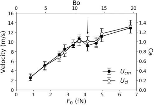
of the drop’s center of mass to determine its velocity with respect to the solid surface 𝑈!". Figure 3 compares the velocity of points on the contact line and the center of mass as a function
of 𝐹! for 𝐶!" = 0.7. It is clear that the velocities are identical. Note that at 𝐹! ~ 3.6 fN the drop begins to elongate and its area of contact with the solid increases. The resulting increase in drag
accounts for the change in slope and the intermediate dip in velocities. The possible significance
Figure 3. Velocities and corresponding capillary numbers Ca of the contact line 𝑈!"! and the
drop’s center of mass 𝑈!" in the 𝑥 directionversus the external force 𝐹! and the associated Bond number for 𝐶!" = 0.7. The arrow marks the force at which the drop begins to elongate.
Raindrops typically have diameters in the range 0.5–5 mm [44]. However, the size of a drop
that will begin to slide down a vertical windowpane depends on the wettability of the glass and
the extent of static contact angle hysteresis. Sliding occurs when the gravitational force exceeds
the capillary resistance caused by the difference between the advancing and receding contact
angles, 𝜃! and 𝜃!, respectively. The gravitational force will scale as 𝜌!𝑔𝑙!, where 𝑔 is the
acceleration due to gravity and 𝑙 is the characteristic size of the drop, whereas the capillary resistance will scale as 𝛾!" cos𝜃!− cos𝜃! 𝑙. Thus, for example, if cos𝜃! − cos𝜃! is order 1, the drop will slide when the Bond number Bo = 𝜌!𝑔𝑙! 𝛾!" > 1, i.e., when 𝑙 > 2.7 mm. Casual
The Bond number scaling law will hold whatever the cause of the difference between 𝜃! and
𝜃!. For simulated Lennard-Jones liquids on an atomistically smooth solid surface, as in our
study, there is no static hysteresis [1,39]. Therefore, drops will begin to slide as soon as a force
is applied, but any consequent changes in the and advancing and receding dynamic contact angle
will have a retarding effect which will increase with speed. Based on our previous simulations
of dynamic wetting [e.g. 27,34–36], we know that the difference between the advancing and
receding dynamic angles can exceed 90˚ for the range of velocities and capillary numbers
depicted in Figure 3. Thus, the expected capillary resistance can easily be of order 𝛾!"𝑙, which is ~ 50 pN for the approximately 20 nm drops used in our study. If we equate this to 𝜌!𝑔!""𝑙!,
where 𝑔!"" represents the effective acceleration supplied by our force, we find that the to
achieve the sliding speeds observed a value of 𝑔!"" is ~ 2 × 10⁹𝑔 is required. During sliding, there will also be significant viscous dissipation, exacerbated by the elongation of the drop, and
we may, therefore, expect the force required to maintain sliding to significantly exceed the
capillary resistance alone. The mass of the smaller drop in our study is 7.97 × 10⁻²² kg, so for the
range of velocities investigated, 𝑔!"" varies from 4.25 × 10⁹𝑔 to 2.55 × 10¹⁰𝑔, which is
consistent with the scaling estimate.
Such high values of 𝑔!"" required to maintain sliding are the inevitable result of the small size of the drops and the consequent increase in the ratio of the perimeter of the drop to its mass when
compared with physical systems. They do not disqualify MD from being used to study the
sliding phenomenon. Precisely because of the small physical scale of the systems that can be
studied, MD provides a consistent approach to aspects of dynamic wetting not directly accessible
by experiment, such as the local microscopic dynamic contact angle and the detailed shape of
simulations, and those of others, have proved entirely effective in recovering standard
macroscopic laws such as the Young and Laplace equations [37,45–47]. Realistic behavior has
also been seen for Poiseuille [48] and Couette flows [26,36]. Another way of comparing our
simulations with the behavior of real drops is to consider the Bond numbers required to maintain
sliding. In the example of the 2.7 mm raindrop given above, sliding commences when Bo > 1. In our simulations, for a 20 nm drop, 0.5 < Bo < 19 for 0.8 < 𝐹! < 6.64 fN, as it can be seen in Fig. 3. The larger values arise because of the relatively low surface tension of our liquid.
3.2 Contact angles.
We determine the local contact angle at points from the slope of the plane tangent to the liquid
interface at a set of points 𝑝! spaced regularly along the contact line. The detailed procedure is
described in Supporting Information. At equilibrium, the contact angle of the drop is the same at
all points along the contact line: 𝜃!. When the drop is moving, the dynamic contact angle
𝜃! depends on the velocity of the contact line normal to itself. Since this varies around the drop,
having maximum and minimum values at the leading and trailing points on the 𝑥 axis, but is zero at equatorial points, the dynamic contact angle should also vary, a result confirmed
experimentally by Rio et al. [39].
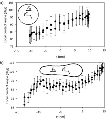
Figure 4 depicts two examples of the variation of the local contact angle with 𝑥 for 𝐶!" = 0.7,
corresponding to an equilibrium angle of 90º. The data are for the lowest and highest forces
studied: 𝐹! = 0.83 and 4.98 fN. The inset figures delineate the actual shape of the contact line in each case. Also indicated are the coordinate systems and their origin, which is at the position of
the mass center projected onto the same 𝑥-𝑦 plane. With 𝐹! = 0.83 fN (Figure 4a), the drop
remains nearly circular and the contact angle increases, nearly monotonically, from a minimum
equilibrium value at the mid-point, where the normal velocity is zero. With 𝐹! = 4.98 fN
(Figure 4b), the larger external force induces much greater deformation of the drop, stretching it
and inducing to a nearly parallel section, where the contact angle is equal to 90º and, therefore,
identical with that of a drop at rest.
Figure 4. Local contact angle versus 𝑥 for 𝐶!" = 0.7. a) 𝐹! = 0.83 fN. b) 𝐹! = 4.98 fN. The
inset figures show the corresponding shape of the contact line, the coordinate system and its
origin.
3.3 Contact-line velocities.
As we have seen, once the drop has reached a steady state under the influence of the applied
same velocity as the center of mass 𝑈!". However, the velocities normal to the contact line vary
with position. If the unit vector normal to the contact line at point 𝑝! is 𝒏 𝑝! the normal
component of the contact-line velocity is the projection of 𝑈!" onto 𝒏 𝑝! :
𝑼𝒄𝒍 𝑝! = 𝑈!" 𝒙 ∙ 𝒏 𝑝! 𝒏 𝑝! = 𝑈!"𝒏 𝑝! . (3)
At the leading and trailing points of the drop 𝑝! and 𝑝!, respectively, (see Figure 2 in Supporting
Information) the normal vectors are 𝒏 𝑝! = 𝒙 and 𝒏 𝑝! = −𝒙, and the contact-line velocity attains its maximum and minimum values, 𝑼𝒄𝒍 𝑝! = 𝑼𝒄𝒍𝒎𝒂𝒙 = 𝑈
!"𝒙 and 𝑼𝒄𝒍 𝑝! = 𝑼𝒄𝒍𝒎𝒊𝒏=
−𝑈!"𝒙, respectively.
In order to compare our results directly with the experiments of Rio et al. [39] for silicone oil
on fluoropolymer treated glass, we may cast our equations in terms of the slope angle of the
contact line 𝜙 with respect to the direction of travel:
𝑈!"sin𝜙 = 𝑈!" 𝒙 ∙ 𝒏 𝑝! . (4)
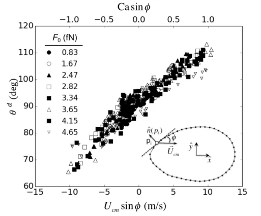
In Figure 5, we plot the dynamic contact angle 𝜃! versus 𝑈
!"sin𝜙 and Ca sin𝜙 at multiple
points around the moving drop for 𝐶!" = 0.7 and all 8 values of 𝐹!. The contact angles are computed in the same way as described for Figure 4. (See Supporting Information). As we can
see, it is possible to determine a wide range of dynamic contact angles from a single sliding drop,
which is a great advantage, both theoretically and experimentally. Significantly for our
understanding of dynamic contact angles, all the points lie close to a single line irrespective of
𝐹!, indicating a common mechanism. The general trend is very like that reported by Rio et al. [39] and Le Grand et al. [18], but without the discontinuity caused by the contact angle
hysteresis present in their experimental system. Another difference is that our results span a
experiments (± 1, compared with ± 0.01) for a comparable range of dynamic contact angles. The range is, however, very similar to that observed previously in comparable simulations of forced
wetting and spreading nanodrops [34-36].
Figure 5. Dynamic contact angle 𝜃! versus 𝑈
!"sin𝜙 and Ca sin𝜙 at multiple points around the
contact line for 𝐶!" = 0.7 and all 8 values of 𝐹! investigated. As shown in the inset, 𝜙 is the angle between the direction of drop travel and the tangent to the contact-line at each point 𝑝!.
3.4 Flow within the drop.
To determine the details of the flow within the sliding drop, we compute the mean local
velocity of the liquid within each of the cubic cells used to determine the local density. We take
two successive saved configurations at times 𝑡 = 𝑡! and 𝑡!+ Δ𝑡. Particle 𝑖, which at time 𝑡! is
𝒖𝒊 = 𝒓𝒊 𝑡!+ Δ𝑡 − 𝒓𝒊 𝑡! Δ𝑡, which is ascribed to both cells 𝑐! and 𝑐!. This procedure is carried out for all the liquid atoms in the drop and all saved configurations separated by Δ𝑡. Thus, we can generate the mean local velocity in each cell and its standard deviation. The value
of Δ𝑡 is chosen to ensure that the displacement of the atoms is not greater than the distance to the next adjacent cell, which maximizes our resolution. Time intervals of Δ𝑡 = 200, 300 and 500 time steps were trialed, which yielded no significant difference in the resulting velocities. Once
the local velocities have been established, the complete flow pattern can be constructed.
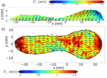
To visualize this, we first consider the flow within the frame of reference of the drop, i.e.,
referenced to its center of mass. Figure 6a shows the flow of the first layer of liquid atoms in
contact with the solid for 𝐶!" = 0.7 and 𝐹! = 3.32 fN, where the color indicates the 𝑥 component
of the velocity. A negative value shows that the liquid moves to the left in the figure, as does the
solid surface in this frame. In all the simulations, there is at least one point on the contact line
where the tangent is parallel to the 𝑥 axis ( = 0º) and the normal velocity of the contact line is zero. Here, the contact angle should have its equilibrium value, as confirmed in Figure 4a and
seen in experiments [39]. The flow in the 𝑥-𝑧 plane, bisecting the drop and passing through its center of mass is illustrated in Figure 6b for 𝐶!" = 0.7 and 𝐹! = 4.98 fN. In this case, the color indicates the 𝑧 component of the velocity and confirms that the drop does not slide but rolls about a stagnation point at its center of mass. However, as can be seen by close inspection of
Figure 6a, the flow within the drop, including that within the first layer, is slower than the
translational velocity of the solid surface in the same frame, −𝑼𝒄𝒎. In other words, there is slip
between the first layer of liquid molecules and the solid. The presence of slip in MD simulations
investigated in its own right [49,50]. We explore its ramifications to our simulations of sliding drops in the next section.
Figure 6. Flow diagrams for 𝐶!" = 0.7, 𝐹! = 3.32 fN, and solid velocity 𝑼𝑺 = −𝑼𝒄𝒎 = 9.3 ±
0.2 m/s. The force 𝐹! acts from left to right in the images. a) flow in the first layer of liquid in contact with the solid. b) flow in the 𝑥-𝑧 plane at the center of the drop. c) the same drop as in a), but now with the velocities referenced to the frame of the solid. d) residual flow when we
[39]. In a), c), and d), the color represents the 𝑥 component of the liquid velocity; in b) the color represents the 𝑧 component of the liquid velocity.
3.5 Slip and contact-line friction.
To quantify the slip between the liquid and the solid, we compare the velocity of the solid
surface relative to the drop, 𝑼𝑺 = −𝑼𝒄𝒎, with that of the first layer of liquid atoms in the central
region of the solid-liquid interface, away from the influence of the contact line. We compute the
velocity of the first layer as follows. We divide the liquid in the 𝑧 direction into arbitrary slices of thickness 𝑧 = 2 nm parallel to the liquid-solid interface. In the central region, the average velocity of the liquid across the center of each slice is 𝑼𝒄 = 𝑈!𝑥, where the modulus of 𝑈! is constant but depends linearly on 𝑧: 𝑈! = 𝑈! 𝑧 . If we define 𝑈!,! as value of 𝑈! 𝑧 ) extrapolated to the solid surface located at 𝑧!, i.e., 𝑈!,! = 𝑈! 𝑧! , the slip velocity in the 𝑥 direction with respect to the solid at the center of the S-L interface is 𝑈!"#$ = 𝑈!− 𝑈!,!. A similar procedure was used in an earlier paper on forced wetting [36]. In Figure 7, we plot the
computed value of 𝑈!"#$ against 𝐹! for the three liquid-solid couplings used in the simulations,
and we can see that the slip velocity increases with the external force, but decreases with
increased coupling, as expected based on current understanding.
To visualize slip and its consequences more directly, Figure 6c, shows the same drop as in 6a,
but now with the velocities referenced to the frame of the solid. We see that all the flow is in the
direction of the applied force, with the highest velocities at the leading and trailing boundaries
where slip is greatest and the velocity is the same as that of the center of mass. However, if we
subtract the local slip velocities then a different picture emerges, as revealed in Figure 6d. Now,
normal to the contact line. This nanoscale flow is consistent with the macroscopic flow observed
in the experiments of Rio et al. [39] for a physical system, as shown in Figure 6e. Thus, it would
appear that for a sliding drop the asymptotic macroscopic flow pattern persists down to the
contact line. Note that in figure 6e the arrow vectors refer to the velocities at the upper surface
of the drop rather than at the solid surface. As the contact line is approached this distinction
becomes irrelevant.
Figure 7. Slip velocity in the central region of the drop 𝑈!"#$ versus 𝐹! for the different S-L
couplings 𝐶!" considered. The dashed lines are linear fits.
As discussed below, slip has a significant effect on the dynamics of the contact line. However,
slip in the 𝑥 direction will affect the normal velocity of the contact line differently according to the peripheral position around the drop, i.e., it will vary with . Hence, the effect will be a
maximum at the front and rear of the drop at points 𝑝! and 𝑝!, where = 90º and -90º,
respectively, but will be zero at intermediate points where = 0. To determine the local effect at each point 𝑝! around the drop, we first compute 𝑼𝒄,𝑺 𝑝! defined as the velocity, in the frame
of the drop, of the first layer of liquid at the center of the S-L interface 𝑈!,!𝒙 projected over the
normal to the contact line at point 𝑝!, 𝒏 𝑝! ; i.e., 𝑼𝒄,𝑺 𝑝! = 𝑈!,! 𝒙 ∙ 𝒏 𝑝! = 𝑈!,! 𝑝! 𝒏 𝑝! =
𝑈!,!𝑠𝑖𝑛𝜙𝒏 𝑝! . Thus, the local slip velocity normal to the contact line will be
𝑼𝒔𝒍𝒊𝒑 𝑝! = 𝑈!"#$ 𝑝! 𝒏 𝑝! = − 𝑈!" 𝑝! + 𝑈!,! 𝑝! 𝒏 𝑝! . (5) Our previous MD studies of dynamic wetting [27,31,32,34–36], and those of others
[28-30,33,37,38] have shown that at the scale of the simulations the dominant cause of the
velocity-dependence of the contact angle is contact-line friction due to the interaction of the liquid
molecules with the potential energy landscape of the solid surface. Many of these studies have
also shown that the molecular-kinetic theory (MKT) of Blake and Haynes [51], further
developed by Blake [52] and Blake and De Coninck [53], provides a good model for the
underlying mechanism. According to the MKT, there is a direct relationship between the
velocity of the contact line normal to itself 𝑈!" 𝑝! and the unbalanced surface tension force
𝛾!" cos𝜃!− cos𝜃! that arises when the dynamic contact angle 𝜃! deviates from its
equilibrium value 𝜃!. If the surface tension is low and/or the interactions with the substrate
fairly weak, as in our simulations, the MKT reduces to a simple linear relation that can be
applied at each point 𝑝! along the contact line:
𝑈!" 𝑝! 𝒏 𝑝! = 𝛾!" cos𝜃!− cos𝜃! 𝜉 𝒏 𝑝
! , (6)
where 𝜉 (Pa·s) is the coefficient of contact-line friction per unit length of the contact line. Since 𝑈!" 𝑝! varies with position around the drop, the local dynamic contact angle 𝜃! must also vary.
In a recent MD study of forced wetting [36], we have shown that the propensity towards slip
between the liquid and the solid has a strong influence on the relationship between the
is reduced by the local slip velocity normal to the contact line: 𝑈!"!"" 𝑝! = 𝑈!" 𝑝! − 𝑈!"#$ 𝑝! . It follows from Eq. (5) that
𝑈!" 𝑝! − 𝑈!"#$ 𝑝! 𝒏 𝑝! = 𝛾!" cos𝜃!− cos𝜃! 𝜉 𝒏 𝑝
! . (7)
To compute the relevant slip velocities, we take the mean of the velocity of the first layer of
liquid across the center of the liquid-solid interface and that at the contact line. This provides a
good estimate of the slip velocity within the small but finite three-phase zone, which constitutes
Figure 8. Unbalanced surface tension force 𝛾!" cos𝜃!− cos𝜃! versus the effective
contact-line velocity 𝑈!"!"" for each value of the external force 𝐹!. a) 𝐶!" = 0.7 (data for small and large drops). b) 𝐶!" = 0.8. c) 𝐶!" = 0.9. The dashed lines indicate the slope of data obtained from simulations of spreading drops at the same S-L couplings [35].
Once we have established the local contact angles and effective contact-line velocities at
multiple points around the moving drops (using the bins as described Supporting Information),
we can use Eq. (7) to calculate the contact-line friction. In each case, the data fall on an
acceptably straight line, from the slope of which we can determine 𝜉. In Figure 8, we plot our results for each solid-liquid coupling 𝐶!" = 0.7, 0.8, and 0.9 versus the external force 𝐹!. As confirmed by the dashed lines in Figures 8 and 9a, the coefficients of contact line friction are
consistent with those found in previous MD simulations of spontaneous spreading of liquid drops
with the same 𝐶!" values [35]. Perhaps the most interesting result is that over the range studied, the contact-line frictions are independent of the external force, and since the contact-line
velocities are measured around the entire circumference of the drop, independent of the local
slope and curvature of the contact line, i.e., they appear to be material properties of the system,
as envisaged by the MKT. Figures 8a and 9a contain the results obtained from the two drop
sizes studied (comprising 5000 and 10643 8-atom molecular chains); thus, it would appear that
the results are not size-dependent at this scale. Indeed, apart from the strength of the liquid-solid
interaction, the only factor that affects the dynamic contact angle is the effective velocity of the
contact line normal to itself. A corollary of this result is that if we know the advancing and
receding dynamic contact angles at the front and rear of the drop, we can predict the angles at all
other points around the drop where the local normal contact-line velocity will be given by
Figure 9. a) Contact-line friction coefficient versus the external force 𝐹! for the three values of
𝐶!" and the two drop sizes investigated. The dashed lines represent the value of the friction coefficient obtained from simulations of spontaneous spreading [35]. b) Apparent friction
coefficient 𝜉!"" computed from the simulations without considering the effect of slip. Here, the
dashed lines represent the average values of the apparent friction coefficient for all values of the
external force.
As shown in Figure 9b, were we not to take account of the slip in our system, i.e., if we were
significantly lower than those observed in the simulations of droplet spreading. As argued
previously [36], the reduction in apparent contact-line friction due to slip induced by the flow is
ultimately because both share the same underlying mechanism, namely the dynamic interaction
of the liquid molecules with the energy landscape of the solid surface. The weaker this
interaction, the smaller the friction and the greater the slip. And the greater the slip, the weaker
the velocity-dependence of the contact angle. As also pointed out, the reduced apparent friction
is a possible source of so-called hydrodynamic assist, whereby liquid coating speeds can be
increased substantially by manipulating the coating flows to avoid air entrainment that follows
when the dynamic contact angle approaches 180º.
3.6 Pearling.
Up to this point, we have considered primarily drops that maintain a simple oval shape.
However, as the external force is increased, the droplet becomes elongated in the direction of
travel: Figures 2d and 2h. If the force is increased still further, then a neck develops between the
front and rear of the drop, which begins to separate into two distinct regions with separate
circulation patterns and an intermediate stagnation zone, as shown in Figures 10a and b. We do
not see a sharp angle at the trailing edge (there is no corner or “cusp”') at the nanoscale. We
therefore suggest that the separation and the inception of the intermediate stagnation zone
provides the microscopic details of the pearling mechanism, i.e., the shedding of droplets, which
is seen at sufficiently high sliding speeds with real macroscopic drops and liquid entrainment on
partially wetted surfaces. If this is the case, then it is helpful to understand at what microscopic
receding contact angle this dynamic wetting transition occurs.
The flow patterns shown in Figure 10 reveal rapid changes in velocity within the tail of the
is the local dynamic contact angle, which we have shown to be velocity dependent, it is of
interest to know how its limiting receding value evolves with 𝐹! and liquid-solid affinity.
Figure 10. Flow diagrams for 𝐶!" = 0.9 and 𝐹! = 3.32 fN showing the development of a neck.
a) Flow in the lateral 𝑥-𝑧 plane along the axis of the drop. The color represents the 𝑧 component of the liquid velocity. b) Flow in the first layer of liquid in contact with the solid. Here, the
color represents the 𝑥 component of the liquid velocity.
Strong affinity leads to a small equilibrium angle and a high friction, but other factors, such as
liquid viscosity, also enhance friction [49,50]. Thus, in principle, one may have a high friction,
but still be in the partially wetting regime. If the friction were sufficiently high, the local
dynamic contact angle might approach zero, leading inevitably to the entrainment of a liquid
film; whereas, if the contact-line friction were comparatively small, the local angle at which the
viscous stresses became dominant would be finite and potentially large, as seen here. One might
dynamic wetting transitions in terms of the way in which the surface free energy of the system
evolves with velocity. However, this requires further investigation.
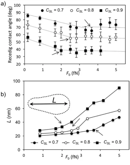
Figure 11a, illustrates the way in which the receding contact angle at the back of the drop
varies with the applied force for the three couplings studied. In each case, we see that beyond a
certain point (indicated by an arrow), which coincides with the appearance of a neck, the contact
angle remains essentially constant at what we interpret to be the critical local dynamic contact
angle for a pearling transition. Beyond this transition, the elongation of the drop simply becomes
more pronounced as 𝐹! is increased. This is illustrated in the plots of drop length 𝐿 versus 𝐹!in Figure 11b. The same transition is also seen in the plot of velocity versus 𝐹! in Figure 3. Presumably, at still higher driving forces, the drop would eventually bifurcate, but our
Figure 11. a) Dependence on 𝐹! of the receding contact angle measured along the 𝑥 axis. b)
Length of drop 𝐿 versus 𝐹!. The arrows show the point at which a neck appears.
In our simulations we measure the local contact angle and find that its value is highly
dependent on the velocity of the contact line. In theoretical investigations of the pearling
transition [2,3,5,16,18,54] this local angle is usually taken to be the equilibrium angle and
invariant, contrary to what we have observed. In experiments, the contact angles are apparent
angles measured with a resolution of a few microns, at a scale greater than that at which viscous
measure the local dynamic angle, but since we see no evidence of viscous bending at the scale of
our simulation, can only infer what effect this will have on the apparent angle at greater scales.
Further progress requires either much larger simulations or multi-scale modelling. Thus far, our
simulations have revealed only forced wetting transitions at finite local angles; but it would
certainly be of interest to investigate the effect of stronger S-L couplings and contact-line
frictions, which would drive the system towards smaller dynamic contact angles.
4. Conclusions
We have performed large-scale molecular-dynamics simulations of nanoscopic liquid drops
moving steadily across a flat solid surface under the influence of a uniform external force field
acting parallel to the liquid-solid interface. Three different liquid-solid affinities and two drop
sizes have been studied at 8 values of the external force 𝐹!. The simulations enable us to extract
the velocity of the contact line normal to itself and the local, microscopic dynamic contact angle
at all points around the drop. In contradiction to the assumptions of existing theoretical models
of sliding drops [2,3,5,16,18,54], we find that the local contact angle measured at this scale
varies continuously, from a maximum advancing angle at the front of the drop to a minimum
receding angle at the rear.
Nevertheless, our results confirm the experimental observation [1,39] that the contact angle is
given by some function of the local contact-line velocity in the normal direction 𝑈!"sin𝜙, where 𝑈!" is the velocity of the drop and 𝜙 is the slope of the contact line with respect to the direction of travel. We also show that this velocity-dependence can be modelled by the molecular-kinetic
theory. A complication is that the simulated drops exhibit slip between the first layer of liquid
molecules and the solid surface. However, once the effects of this are included, the contact-line
spreading drops. Moreover, despite the small scale of the simulations, flow within the drop with
respect to the solid surface is consistent with that observed by Rio et al. [39] and Le Grand et al.
[18] in macroscopic experiments.
If the external force is increased beyond a certain value then the nanodrop elongates, its
velocity increases more slowly with 𝐹! and a neck appears between the front and rear of the drop, which separates into two distinct zones. We suggest that this indicates the nanoscale
mechanism of the pearling transition at the tip of a macroscopic drop. While the receding
contact angle at this hydrodynamic transition is far removed from its equilibrium value, it is
greater than zero and approaches a more-or-less constant value as the transition progresses. It
would appear that this angle provides a system-specific critical condition for pearling. We
conclude, therefore, that any complete theory of dynamic wetting transitions and associated
avoided critical behavior at any scale should consider the impact of a velocity-dependent local
microscopic contact angle.
Acknowledgment
This research was partially funded by the Interuniversity Attraction Poles Programme (IAP
7/38 MicroMAST of the Belgian Science Policy Office). Computational resources have been
provided by the Consortium des Equipements de Calcul Intensif (CECI), funded by the Fonds de
la Recherche Scientifique de Belgique (F.R.S.-FNRS) under Grant No. 2.5020.11. One of us
(LL) acknowledges FNRS and UMONS for some financial support and Labex SEAM (Science
and Engineering for Advanced Materials and Devices), contracts LABX-086,
ANR-11-IDEX-05-02 with Agence National de la Recherche and Commissariatà l'Investissement d'avenir,
[1] T.D. Blake, K.J. Ruschak, A maximum speed of wetting, Nature 282 (1979) 489–491.
[2] L. Limat, H.A. Stone, Three-dimensional lubrication model of a contact line corner
singularity, Europhys. Lett. 65 (2004) 365–371.
[3] J.H. Snoeijer, E. Rio, N. Le Grand, L. Limat, Self-similar flow and contact line geometry
at the rear of cornered drops, Phys. Fluids 17 (2005) 72101.
[4] L.W. Schwartz, L. D. Roux, J.J. Cooper-White, On the shapes of droplets that are sliding
on a vertical wall, Phys. D Nonlinear Phenom, 209 (2005) 236–244.
[5] J.H. Snoeijer, N. Le Grand-Piteira, L. Limat, H.A. Stone, J. Eggers, Cornered drops and
rivulets, Phys. Fluids 19 (2007) 42104.
[6] I. Peters, J.H. Snoeijer, A. Daerr, L. Limat, Coexistence of two singularities in dewetting
flows: Regularizing the corner tip, Phys. Rev. Lett. 103 (2009) 103 114501.
[7] T.D. Blake, The physics of moving wetting lines, J. Colloid Interface Sci. 299 (2006) 1–13.
[8] D. Bonn, J. Eggers, J. Indekeu, J.Meunier, E. Rolley, Wetting and spreading, Rev. Mod.
Phys. 81 (2009) 739–805.
[9] W. Ren, D. Hu, W. E, Continuum models for the contact line problem, Phys. Fluids 22
(2010) 102103.
[10] E. Bertrand, T.D. Blake, J. De Coninck, Dynamics of dewetting, Colloids Surfaces A
Physicochem. Eng. Asp. 369 (2010) 141–147.
[11] J.H. Snoeijer, B. Andreotti, Moving contact lines: Scales, regimes, and dynamical
[12] R.V. Sedev, J.G. Petrov, The critical condition for transition from steady wetting to film
entrainment, Elsevier Sci. Publ. B.V Amsterdam 53 (1991) 147–156 .
[13] D. Quéré, On the minimal velocity of forced spreading in partial wetting, C. R. Acad. Sci.
Paris II 313 (1991) 313–318.
[14] J.H. Snoeijer, G. Delon, M. Fermigier, B. Andreotti, Avoided critical behavior in
dynamically forced wetting, Phys. Rev. Lett. 96 (2006) 174504.
[15] G. Delon, M. Fermigier, J.H Snoeijer, B. Andreotti, Relaxation of a dewetting contact line.
Part 2. Experiments, J. Fluid Mech. 604 (2008) 55–75.
[16] T. Podgorski, J.-M. Flesselles, L. Limat, Corners, cusps, and pearls in running drops, Phys.
Rev. Lett. 87 (2001) 36102.
[17] H.-Y. Kim, H.J. Lee, B.H. Kang, Sliding of liquid drops down an inclined solid surface, J.
Colloid Interface Sci. 247 (2002) 372–380.
[18] N. Le Grand, A. Daerr, L. Limat, Shape and motion of drops sliding down an inclined
plane, J. Fluid Mech. 541 (2005) 293–315.
[19] K.J. Winkels, I.R. Peters, F. Evangelista, M. Riepen, A. Daerr, L. Limat, J.H. Snoeijer,
Receding contact lines: From sliding drops to immersion lithography, Eur. Phys. J. Spec.
Top. 192 (2011) 195–205.
[20] L. Limat, Drops sliding down an incline at large contact line velocity: What happens on the
road towards rolling? J. Fluid Mech. 738 (2014) 1–4.
(2015) 23008.
[22] P. Gao, L. Li, J.. Feng, H. Ding, X.-Y. Lu, Film deposition and transition on a partially
wetting plate in dip coating, J. Fluid Mech. 791 (2016) 358–383.
[23] J. Koplik, J.R. Banavar, J.F. Willemsen, Molecular dynamics of Poiseuille flow and
moving contact lines, Phys. Rev. Lett. 60 (1988) 1282–1285.
[24] P.A. Thompson, M.O Robbins, Simulations of contact-line motion: Slip and the dynamic
contact angle, Phys. Rev. Lett. 163(1989) 766–769.
(25) J. Koplik, J.R. Banavar, J.F. Willemsen, Molecular dynamics of fluid flow at solid
surfaces, Phys. Fluids A Fluid Dyn. 1 (1989) 781–794.
[26] P.A. Thompson, W.B. Brinckerhoff, M.O Robbins, Microscopic studies of static and
dynamic contact angles, J. Adhes. Sci. Technol. 7 (1993) 535–554.
[27] M.J. de Ruijter, T.D. Blake, J. De Coninck, Dynamic wetting studied by molecular
modeling simulations of droplet spreading, Langmuir 15 (1999) 7836–7847.
[28] D.R. Heine, G.D. Grest, E.B. Webb III, Spreading dynamics of polymer nanodroplets,
Phys. Rev. E 68 (2003) 61603.
[29] T. Qian, X-P. Wang, P. Sheng, Molecular scale contact line hydrodynamics of immiscible
flows, Phys. Rev. E. 68 (2003) 016306.
[30] D.R. Heine, G.S. Grest, E. B. Webb III, Spreading dynamics of polymer nanodroplets in
cylindrical geometries, Phys. Rev. E 2004, 70, 11606.
Langmuir 20 (2004) 8385–8390.
[32] E. Bertrand, T.D. Blake, V. Ledauphin, G. Ogonowski, J. De Coninck, D. Fornasiero, J.
Ralston, Dynamics of dewetting at the nanoscale using molecular dynamics, Langmuir
2007, 23, 3774–3785.
[33] W. Ren, W.E, Boundary conditions for a moving contact line problem, Phys. Fluids 19
(2007) 022101.
[34] E. Bertrand, T.D. Blake, J. De Coninck, Influence of solid–liquid interactions on dynamic
wetting: a molecular dynamics study, J. Phys. Condens. Matter. 21 (2009) 464124.
[35] D. Seveno, N. Dinter, J. De Coninck, Wetting dynamics of drop spreading. New evidence
for the microscopic validity of the molecular-kinetic theory, Langmuir 26 (2010) 14642–
14647.
[36] T.D. Blake, J.-C. Fernandez-Toledano, G. Doyen, J. De Coninck, Forced wetting and
hydrodynamic Assist, Phys. Fluids 27 (2015) 112101.
[37] A.V. Lukyanov, A.E. Likhtman, Dynamic contact angle at the nanoscale: a unified view,
ACS Nano 10 (2016) 6045–6053.
[38] A.V. Lukyanov, T. Pryer, Hydrodynamics of moving contact lines: Macroscopic versus
microscopic, Langmuir 33 (2017) 8582–8590.
[39] E. Rio, A. Daerr, B. Andreotti, L. Limat, Boundary conditions in the vicinity of a dynamic
contact line: Experimental investigation of viscous drops sliding down an inclined plane,
[40] E. Salomons, M. Mareschal, Surface tension, adsorption and surface entropy of
liquid-vapour systems by atomistic simulation, J. Phys. Condens. Matter 3 (1991) 3645–3661.
[41] A. Einstein, Investigations on the theory of the Brownian movement, Dover, 1956.
[42] D.J. Allen, M.P. Tildesley, Computer simulation of liquids, Oxford: Clarendon Press,
1987.
[43] M. Wilczek, W. Tewes, S. Engelnkemper, S.V. Gurevich, U. Thiele, Sliding drops:
Ensemble statistics from single drop bifurcations, Phys. Rev. Lett. 119 (2017) 204501.
[44] Lenard, P. Translations of five raindrop size and velocity studies, Meteorol. Z. 21 (1904)
248–262.
[45] J.-C. Fernandez-Toledano, T.D. Blake, P. Lambert, J. De Coninck, On the cohesion of
fluids and their adhesion to solids: Young’s equation at the atomic Scale, Adv. Colloid
Interface Sci. 245 (2017) 102–107.
[46] J.-C. Fernandez-Toledano, T.D. Blake, J. De Coninck, Young’s equation for a two-liquid
system on the nanometer scale, Langmuir 33 (2017) 2929–2938.
[47] D. Seveno, T.D. Blake, J. De Coninck, Young’s equation at the nanoscale, Phys. Rev. Lett.
111 (2013) 1–4.
[48] G. Martic, F. Gentner, D. Seveno, J. De Coninck, T.D. Blake, The possibility of different
time scales in the dynamics of pore imbibition, J. Colloid Interface Sci. 270 (2004) 171–
179.
surfaces, Nature 389 (1997) 360–362.
[50] N.V. Priezjev, Rate-dependent slip boundary conditions for simple fluids, Phys. Rev. E -
Stat. Nonlinear, Soft Matter Phys. 75 (2007) 051605.
[51] T.D. Blake, J.M. Haynes, Kinetics of liquid/liquid displacement, J. Colloid Interface Sci.
30 (1969) 421–423.
[52] T.D. Blake, Dynamic contact angles and wetting kinetics, in: Wettability, Ed. J.C. Berg,
Marcel Dekker, 1993: pp. 252–309.
[53] T.D. Blake, J. De Coninck, The influence of solid–liquid interactions on dynamic wetting,
Adv. Colloid Interface Sci. 96 (2002) 21–36.
[54] J. Eggers, Hydrodynamic theory of forced dewetting, Phys. Rev. Lett. 93 (2004) 94502.
Supporting Information
S1. Finding the density and position of the liquid-vacuum interface.
To calculate the density of the liquid for each position vector 𝜌!𝒓𝒊(𝑡), we subdivide the available volume of the drop into cubic cells of size 𝑑𝑥, 𝑑𝑦, 𝑑𝑧 = 0.3 nm and calculate the average number of atoms per cell over 500 configurations at intervals of 103 time steps. From
these we extract 10 independent density profiles, which we use to establish the location of the
interface, the position of the contact line, the local contact angles, and the associated errors. The
drop is sliced into 𝑘 layers parallel to the L-S interface, as shown in Figure S1a. The density in each slice depends on the 𝑥-𝑦 coordinates; therefore, we decompose the slices into bins perpendicular to the 𝑥 axis, as indicated in Figure S1b and compute the density profile along the 𝑦 coordinate. A typical example is shown in Figure S1c. Finally, this profile is split into two
symmetrical regions about the 𝑥 axis and we fit sigmoidal functions to determine the position of the interface where the density falls to half that of the bulk liquid. This is done for each slice in
the 𝑧 direction to locate the complete liquid-vacuum interface.
Figure S1. a) Density map profile for 𝐶!" = 0.7 and 𝐹! = 3.3 fN computed in the 𝑥-𝑧 plane which cuts the mass center of the drop. The region contained between the two parallel lines
represents an arbitrary layer 𝑘. b) Density map of the selected 𝑘-layer in a) in the 𝑥-𝑦 plane. c) Density profile versus 𝑦, together with the fit and the interface location (marked with crosses) of the selected bin 𝑗 of b).
S2. Measuring the local contact angle.
We determine the local contact angle from the slope of the plane tangent to the liquid-vacuum
interface at a set of points 𝑝! spaced regularly along the contact line. The first step is to establish the normal to the contact line at each point 𝑝! = 𝑥!, 𝑦! , which is defined by 𝑦 = 𝑦!−
Next, we calculate the point of intersection of this normal with the 𝑥-𝑦 projection of the liquid-vacuum interface obtained from the 𝑘 slices along 𝑧, (𝑧!, 𝑧!, … , 𝑧!), as shown in Figure S2a.
The normal at each point 𝑝! on the contact line intersects the projection of each layer 𝑘 at 𝑝! = 𝑥!, 𝑦!, 𝑧! and the interfacial profile is given by 𝑧! as a function of the distance in the 𝑥-𝑦 base plane 𝑟 = 𝑥!− 𝑥! !+ 𝑦
! − 𝑦! !. Finally, a circular arc is fitted to the profile omitting
the first two layers of atoms in contact with the solid, as illustrated in Figure S2b, and we
measure the contact angle as the tangent to this arc at its intersection with the solid. The mean
value and standard deviation of each contact angle is calculated by repeating this procedure for
the 10 density profiles determined as described above.
Figure S2. a) Calculation of the normal to the contact line at the point 𝑝𝑖 and its intersection with the projection of the L-V interface for a sequence of layers on the base plane. b) Interfacial
profile computed along the normal shown in a) and its circular fit to give the local dynamic
contact angle 𝜃! 𝑝