HAL Id: halshs-01254729
https://halshs.archives-ouvertes.fr/halshs-01254729
Submitted on 12 Jan 2016
HAL is a multi-disciplinary open access
archive for the deposit and dissemination of sci-entific research documents, whether they are pub-lished or not. The documents may come from teaching and research institutions in France or abroad, or from public or private research centers.
L’archive ouverte pluridisciplinaire HAL, est destinée au dépôt et à la diffusion de documents scientifiques de niveau recherche, publiés ou non, émanant des établissements d’enseignement et de recherche français ou étrangers, des laboratoires publics ou privés.
Liquidity and Equity Short term fragility: Stress-tests
for the European banking system
Guillaume Arnould, Catherine Bruneau, Zhun Peng
To cite this version:
Guillaume Arnould, Catherine Bruneau, Zhun Peng. Liquidity and Equity Short term fragility: Stress-tests for the European banking system. 2015. �halshs-01254729�
Documents de Travail du
Centre d’Economie de la Sorbonne
Liquidity and Equity Short term fragility: Stress-tests for the European banking system
Guillaume ARNOULD, Catherine BRUNEAU, Zhun PENG
Liquidity and Equity Short term fragility:
Stress-tests for the European banking system
∗Guillaume Arnould
†1, Catherine Bruneau
‡1, and Zhun Peng
§21University Paris I Pantheon-Sorbonne and CES 2University of Evry and EPEE
Abstract
This paper investigates the impact of extreme shocks on stock and bond markets on listed European banks. The originality of our approach consists in dealing jointly with stock and bond markets and taking into account their interdependencies in case of extreme events by using a specific CVRF (CVine Risk Factor) model which combines copulas and a factorial structure. Moreover, contrary to what is generally done in the literature, we do not focus only on the responses of the stock returns but we also examine the response of the balance sheets of the banks and particularly of their short term assets in order to assess their fragility in terms of liquidity. Our main findings are the following: 1) the nature of the banks’ fragility has changed: today, the interest rate risk should be the first concern before the equity risk, as the banks have extensively increased their exposition to bond market due to flight-to-quality reactions and to large investments in governments bonds after the rescue operations the banks have benefited; 2) in case of a surge in the interest rate and in the links between stock and bond returns, the portfolios of the biggest banks in Europe would experience very severe shortfalls for both equity and liquidity buffers. Accordingly regulators should monitor the evolution of dependencies between as-sets and should pay utmost attention to the positive links between stock and bond returns.
Keywords: Stress-test, Financial Stability, Extreme Risks, Bank Balance Sheet, Systemic Risk, Copula, Risk factors.
JEL classification: F32, G17, G21
∗ This work was achieved through the Laboratory of Excellence on Financial Regulation (Labex
ReFi) supported by PRES heSam under the reference ANR-10-LABX-0095. It benefitted from a French government support managed by the National Research Agency (ANR) within the project Investissements d’Avenir Paris Nouveaux Mondes (investments for the future Paris-New Worlds) under the reference ANR-11-IDEX-0006-02.
†106-113 Bd de l’Hˆopital 75013 Paris, France. guillaume.arnould@univ-paris1.fr
‡106-113 Bd de l’Hˆopital 75013 Paris, France. catherine.bruneau-chassefiere@univ-paris1.fr
1
Introduction
Since the last crisis, stress-testing has become a key supervisory tool. It has been used frequently by the Federal reserve since 2008 and is now widespread among developed countries as demonstrated by the stress-testing exercise conducted by the ECB (ECB, 2014) in the end of 2014. However these stress-tests focus on the impact of extreme scenarios on banks’ equity leaving behind the liquidity issue (Arnould and Dehmej, 2015). However banks highly rely on wholesale funding as it represents 61% of their liabilities (IMF-GFRS, 2013). This funding is particularly prone to volatility and plays a central role in transmitting shocks from the financial markets to the banks (Babihuga and Spaltro, 2014). As shown by the Northern Rock bankruptcy, wholesale funding and particularly short term one is a major source of fragility. Lopez-Espinosa and al. (2013) even claim that unstable funding is the most significant factor driving solvency risk and systemic risk.
The short term sensitivity of a bank to a shock on financial markets depends on two buffers: the equity buffer and the liquidity buffer. The first one is expected to absorb losses and to allow the bank to continue to operate. The second one represents available assets, offsetting the usual and additional repayments that may arise over a defined short period of time under stress conditions. More precisely, it is the difference between liquid assets that can be sold to repay a debt and short term debt which must be frequently rolled-over or can be redeemed on short notice.
The approach we adopt enables us to implement stress test exercises on banks’ short term balance sheet in order to develop a comparative analysis of banks’ individual expo-sitions to market risks through the two buffers of equity and liquidity.
One part of the literature focuses on the equity buffer as, for example, Brownlees and Engle (2015) with the SRISK which is the conditional capital shortfall of a bank under a shock to the stock market. Another part focuses on banks’ liquidity position, like (Brunnermeier et al., 2012), who develop the Liquidity Mismatch Index which by assigning a liquidity level for each item of a bank’s balance sheet, can compare the global liquidity of the assets and the one of the liabilities. Both buffers are linked : a strong
equity buffer makes run on short term debt less likely and, conversely, a stronger liquidity buffer makes banks more resilient and can lower the price of newly emitted equity. To our knowledge, few papers have tried to link the two sides. Pierret (2015) show that the SRISK is positively related to the book liquidity position of the bank but doesn’t investigate the link.
In this paper we also aim at linking market equity buffer with market liquidity buffer but also investigate the nature of the link, in order to give a exhaustive view of bank’s short term fragility. More precisely we use detailed balance sheet of 38 listed European banks, on the period 2005-2014, to build an equity buffer and a liquidity buffer. We use the market value of the bank as the equity buffer as in Brownlees and Engle (2015). For the liquidity buffer we relate to the liquidity ratios defined by Basel regulation (BCBS , 2014) which build a ratio between short term assets and short term debt, namely the LCR (Liquidity Coverage Ratio). We consider an asset to be of short term if it is a trading asset held for trading, a derivative, or a very liquid assets (such as central bank cash). The short term debt comprises all debt with a residual maturity less than one year (senior or covered bonds) and wholesale funding that must be frequently rolled over or can be redeemed on short notice (for example: bank deposits or deposits maturing in less than 3 months). Followig Kahlert and Wagner (2015), we define 4 major sources of market risk (equity, rate, commodity and foreign exchange) each item of our buffers (either assets or liabilities) are assigned to an appropriate risk sources in order to evaluate their fair value in case of a shock on one of our source of risk.
Then we construct the structure of dependencies between the sources of risk and the item of our buffers, using a Cvine Risk Factors Model (CRFM) model as Bruneau et al. (2015), which combines copulas and factors. We account for changes in the dependence structure by using rolling windows in the estimation procedure. A particular advantage of the CRFM framework lies in its ability to capture the tail dependencies for a large number of assets, directly or indirectly through the factorial structure and to allow for second round contagion. Over the period 2005-2014, our estimation results indeed reveal tail dependencies of the retained common risk factors as displayed by Kendall’s taus and
more specifically by the types of copulas and their parameters. Moreover we observe clear changes in the dependence structure over time. Thanks to the modeling of the interconnections between all source of risk, we are able to capture the indirect effects of any global shock. For example, a shock on the index representative of the rate risk impacts not only the bonds but also the equity, due to the link between this factor and the market factor accounting for the stock market risk. We simulate shocks on market indexes representing our 4 sources of risk and examine how the banks’ buffers of equity and liquidity that we built respond.
We find that Bank’s solvability and liquidity fragility are intertwined, as outlined by Pierret (2015). We observe that trading portfolio are quite sensitive to equity shocks with significant potential losses. We also find that the banks of our panel still display large fragility even if the liquidity position at the aggregate level has improved during the considered period (2005-2014). If we look more closely, we observe that banks of intermediate size are the most robust to shocks on the equity Risk Index and to rate Risk Index concerning both equity and liquidity buffers, while the liquidity position of the smallest banks has not improve and remains insufficient. Concerning the equity risk, we find that it affects the largest banks almost exclusively. We also find that french banks are among the most fragile for the recent period, displaying large shortfalls on both buffers whatever the source of the shock.
We want to stress that the nature of fragility has changed since the last crisis: before the crisis, the banks were mainly exposed to the equity risk, while their major fragility come today from their massive exposure to the interest rate risk.
The latter finding is particularly important if one thinks of the impact that the end of Quantitative Easing could have on the banking system. Indeed, by performing a stress test with a joint increase in the level of the interest rate and in the interdependencies between the equity and bond markets, we find that the portfolios of the biggest banks in Europe would need e500 billions and e100 billions for the liquidity and equity buffers respectively, which represent striking shortfalls if one notes that the shock to the rate is rather small and already occured in our sample period.
The structure of the paper continues as follows. In section 2 we present the economet-ric methodology and the construction of the buffers from the short term balance sheet. In Section 3 we present the data . Section 4 documents the results based on the three identified dimensions (bank’s portfolio, dependencies and shocks). Section 5 concludes.
2
Methodology
2.1
Econometric Methodology
In this section we present our econometric modeling by recalling first the principles of a CVRF model and explaining then how simulations are run for the stress test exercises, before turning to the measures of the equity and liquidity buffers deduced from the balance sheet.
2.1.1 Model estimation
Sklar’s theorem (Sklar, 1959) states that any multivariate joint distribution of n random variables X = (X1, ..., Xn) can be written in terms of univariate marginal distribution
functions F1(x1),...,Fn(xn) and a copula which describes the dependence structure
be-tween the variables:
F (x1, ..., xn) = C(F1(x1), ..., Fn(xn)) = C(u1, ..., un)) (1)
where F denotes the cumulative distribution function (cdf) of the n variables and C(.) is some appropriate (uniquely defined) n-dimensional copula which is a cumulative dis-tribution function (cdf) with uniformly distributed marginals Ui = Fi(Xi) on [0,1].
Accordingly, modeling of margins and dependence can be separated. Moreover, for an absolutely continuous F with strictly increasing, continuous marginal cdf Fi, we get
the joint density function f by differentiating (1),
which is the product of the n-dimensional copula density c1:n(·) and the marginal densities
fi(·).
Finally, the n−dimensional density c1:n can be decomposed as a product of bi-variate
copulas. The decomposition is not unique. To help organize the possible factorization of the joint density, Bedford and Cooke (2001, 2002) have introduced a graphical model denoted the regular vine. Regular vines (R-vines) are a convenient graphical model to hierarchically structure pair copula constructions. A special case of regular vines is the canonical vine where certain variables play a leading role.
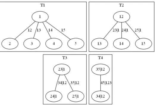
Figure 1 shows a canonical vine with five variables. From the figure, we observe that the variable 1 at the root node is a key variable that plays a leading role in governing interactions in the data set.
Figure 1: A five dimensional canonical vine tree
In the first tree, all nodes are associated with the X1, ..., X5 variables. For example,
the edge 12 corresponds to the copula c(F1(x1), F2(x2). In the second tree, the edge 23|1
denotes the copula c(F2|1(x2|x1), F3|1(x3|x1)). The following trees are built according to
the same rules. In what follows, the Xi variables are asset returns.
To get a CVFR model we have to combine a factorial structure to a C-vine. This is achieved by imposing dependency constraints in the lines of Heinen and Valdesogo
Table 1: Factorial dependence matrix Ms F1 F2 F3 F4 a1 a2 a3 a4 F1 1 F2 1 1 F3 1 0 1 F4 1 0 1 1 a1 1 1 0 0 1 a2 1 1 1 0 0 1 a3 1 0 1 1 0 0 1 a4 1 0 1 1 0 1 0 1
(2009) who build a CVMS (C-Vine Market-Sector) model to describe the dependence structure between asset returns mainly driven by market and sectors. We assume that asset returns share several common risk factors -possibly interconnected- which mainly explain their dependence structure so that they are independent when taken conditionally on the factors.
Generally speaking, for a set of conditioning variables, υ and two variables X, Y , assuming that X and Y are conditionally independent given υ, is equivalent to:
cxy|υ(Fx|υ(x|υ), Fy|υ(y|υ)) = 1. (3)
where cxy|υ denotes the copula describing the dependence structure of X and Y taken
conditionally on υ.
Thus combining a factorial structure with a C-vine reduces to specify a dependence matrix Ms with elements equal to 0, in case of independence and 1 otherwise as in table
1 for example.
Among the n = 8 assets associated with the previous table, we distinguish between F -type assets which are Factors1 and a-type ones which refer to the other assets of
the database (stocks, bonds, currencies..). The random variables are the corresponding returns, ri, i = 1, ..., 8. If the element ij of the matrix is equal to 1, the return of asset
aj (or of market factor M Fj) is related to the return of asset ai (or common component
M Fi), conditionally on the returns of any asset (or common component) preceding aj
(e.g., rj−1,rj−2,...,r1). If this element is equal to 0, the pair is conditionally independent
and the density of the associated copula is equal to one.
Specifying the previous matrix Ms allows us to impose any dependence structure
specified “a priori”. All diagonal entries are equal to 1 since each asset is obviously linked with itself, but imposing that all elements of the first column are equal to 1 means that the returns of all assets (including the ones of the common components F2, F3 and F4)
depend on the first Factor F1. We can impose conditional independence or dependence
between the Factors; here, elements M(3,2)s and M(4,3)s are respectively equal to 0 and 1, meaning that F2 and F3 are independent, conditionally on F1, while F4 and F3 are
dependent, conditionally on F1.
Moreover, each asset can share just one Factor as well as several ones: for example, a1
is only related to F2 conditionally on F1 while a3 is related to F3 and F4, conditionally on
F1. In the same way, assets can be dependent or independent on each other conditionally
on the Factors: for example, element M(8,6)s is equal to 1 which means that a2 is related
to a4 given the 4 Factors while M(8,7)s = 0 indicates that a3 and a4 are conditionally
independent. Moreover, for each pair of assets (i, j), such that Ms
(i,j)= 1, the dependence
is further characterized by one copula chosen among various bivariate copulas.
Once specified the dependence matrix, we proceed in two steps. First we estimate the marginal distributions of the returns. Different approaches are possible. Here we retain the empirical distributions. Then, according to:
Ui = Fi(Xi) (4)
for i = 1, ..., n, each return ri is transformed into a uniform “residual” ui by using the
empirical cumulative distribution functions Fi as in Meucci (2007).
In a second stage, we fit a Canonical Vine (C-Vine) copula structure to the uniform residuals ui, i = 1, ..., n, and, more precisely, we fit bivariate copulas to all pairs of these
uniform residuals whilst taking into account the factorial dependence structure specified by the matrix Ms. The bivariate copulas are thus chosen from a set of copula families:
2.1.2 Simulation
In the following we describe two types of simulations that allow us to perform stress tests. To run the simulations, we proceed as follows. First, by using the different bivari-ate copulas chosen at the estimation step and the corresponding estimbivari-ated parameters, we implement the algorithm described in (Aas et al., 2009) to get N samples from the n dimensional canonical vine C for the next period, i.e. ˆUi,T +1by taking into account the
de-pendence constraints imposed through the matrix Ms. Then, the inverse empirical
cumu-lative distribution functions (Fi−1) provides a sample of returns, i.e. ˆri,T +1 = Fi−1(ˆui,T +1)
for i = 1, ..., n.
For simulations under extreme shocks, we impose that the return of one particular asset i among the n assets has an extreme behaviour by constraining the corresponding uniform residual ˆui to belong to an extreme zone, for example ˆui ≤ 0.01; the extreme
shock thus concerns asset i and, by using the algorithm proposed in Brechmann et al. (2013), we draw samples from the C copula conditionally on an extreme value of ˆui.
Since the dependence structure is supposed to be unaffected by the shock, a stress situation for one asset impacts not only the assets whose returns are directly related to the return of the stressed asset but also the other returns in an indirect way, by affecting the key variable at the root node of the C-Vine (which is related to all returns). This means that a sharp decrease in the return of one market factor (the stressed asset) can cause the distress of a bank if the assets of the banks are positively related to the market factor. Conversely, in the case where some assets are negatively related to the stressed market factor, the bank can benefit from diversification effects and be less affected by the shock than isolated assets.
2.2
Short term balance sheet
For a bank i at time t, the bank balance sheet is divided between short term, long term assets and liabilities, and equity:
With ST Ait denoting the market value of short term assets, ST Dit, the market value
of short term liabilities, Wit, the market value of equity, LT Ait the book value of long
term assets and LT Dit the book value of long term liabilities for a bank with index i.
We define two buffers, one of equity Eqit and one of liquidity Liqit :
Eqit = Wit/(ST Ait+ LT Ait) (6)
Liqit = ST Ait/ST Dit (7)
The former is a leverage ratio, meaning a ratio between the equity of the bank and its total assets. It indicates the solvability of the bank, its ability to withstands losses on its operations. The latter is the ratio between its short term resources (ST Ait) and
its short term debt (ST Dit) and figures the ability of a bank to fulfill it’s short term
commitments.
We rely on Basel III requirements (BCBS , 2011) to set the prudential ratios banks have to comply with. Contrary to Brownlees and Engle (2015), we set the capital re-quirement to 3% as required for the leverage. Concerning our liquidity buffer Liqit, we
consider the Liquidity Coverage Ratio as defined in BCBS (2014), and set a 100% ratio.
Wit/(ST Ait+ LT Ait) ≥ 3% (8)
ST Ait/ST Dit≥ 100% (9)
Then we generate a set of k short term shocks (Ck) to the bank’s balance sheet, which
spreads to the bank’s balance sheet composed of market assets or liabilities, namely Wit,
ST Ait and ST Dit. Since LT Ait and LT Dit are long term items (over 1 year), we assume
that they are not affected by those short term shocks, and that their value is kept constant at this short term horizon. The expected values of our buffers affected by the shocks, which appears through conditional expectations one period ahead:
Et(Wit+1|Ck)
Et(ST Ait+1|Ck) + LT Ait)
Et(ST Ait+1|Ck)
Et(ST Dit+1|Ck)
≥ 100% (11)
As a consequence of the shock, the bank may have to recapitalize if Et(Eqit + 1|Ck) ≤
3% or to protect itself against the risk of illiquidity if Et(Liqit + 1|Ck) ≤ 100%, either by
selling long term assets, or by decreasing its dependence on short term funding. We can already notice that the equity and buffer and the liquidity buffer are connected through Et(ST Ait+1|Ck) which has opposite effect (its increase reinforce Liqit but is detrimental
to Eqit).
3
Data
The sample period for data ranges from January 2005 to December 2014. It covers several crises (the Great Recession and Eurozone sovereign debt crisis) but also less volatile periods such as 2005-2006 or 2013-2014. We use 17 financial market series all extracted from Bloomberg and the balance sheet of 35 banks from 11 countries extracted from SNL (see Appendix 6.1).
3.1
Market data
We have cut down the various risks a bank is exposed to six as in Kahlert and Wagner (2015), which we believe allow us to have an exhaustive and parsimonious view of banks’ risks. We associate a financial series to each of those Risk Indexes (Table 2).
Table 2: Risk Indexes
Market series Risk Index Eurostoxx (TR) Equity
Bobl2 Interest Rate
Iboxx euro Sov Sovereign Iboxx euro Corp Corporate
EUR-USD exchange rate Foreign exchange DJUBS Commodity Commodities
The ranking of our Risk Indexes puts equity Risk Index in the first place instead of the rate Risk Index, unlike Bruneau et al. (2015), since financial markets are primary drivers
of risks contagion through the agents’ expectations (Cappiello and al., 2006). We also add 11 series of national stock indexes to control for country specific risk (see Appendix 6.2).
All the data are extracted from Bloomberg. We work with the weekly returns (as of Fridays) of the 17 market indexes. We report some descriptive statistics for the 6 Risk Indexes in Table 33. We observe that the equity and commodity Risk Indexes are more volatile than the other Risk Indexes. Positive kurtosis indicate that the distributions of the six index returns have fat tails. The distributions of equity, Euro Corporate bond, currency and commodity indexes are asymmetric, as indicated by the negative skewness, and have longer left tails as indicated by the values of the minimal return and the kurtosis, which means that extreme negative returns are relatively more frequent.
Table 3: Descriptive statistics
Eurostoxx Bobl Iboxx euro sov Iboxx euro Corp EUR-USD exchange rate DJUBS Commodity Min -22.22% -1.36% -2.07% -3.13% -5.69% -13.57% Max 12.21% 1.62% 3.02% 2.03% 5.51% 6.48% Mean 0.06% 0.05% 0.09% 0.08% -0.01% -0.02% Median 0.37% 0.05% 0.12% 0.12% -0.02% 0.15% Std. Dev. 0.14% 0.02% 0.02% 0.02% 0.06% 0.11% Skewness -0.88 0.10 0.23 -0.61 -0.14 -0.86 Kurtosis 6.31 0.65 2.67 4.83 1.67 2.95
We also collect weekly returns of each bank’s stock on the same period (January 2005 to December 2014). Market value of banks are not a perfect substitute for the real book value of capital of a bank as Tavolaro and Visnovsky (2014) points out, but allow us to have direct and dynamic dependencies and is widely used as an imperfect substitute.
3.2
Balance sheet data
The banks of our panel are those that took part to the AQR and stress-test conducted by the ECB in 2014 and are listed. There are 38 such banks as in Acharya and Steffen
3We tried alternative series such as ”World MSCI Index” the characterize the Equity risk or “Citi
Germany GBI 3-7 Yr Index” to account for the Rate risk without changing very much the dimension of dependencies or shocks.
(2014). We have continuous data for 354 of them (see Appendix 6.3). Our sample yields
for 40% of all the assets of Eurozone 5 monetary and financial institutions (Table 4). In
details, our sample ranges from 89% do 6% of national MFIs total assets. Despite the fact that Italian banks yields for almost one third of our sample in term of number of banks, it is the French banking system that trusts the bigger share with 35% (next comes Germany at 20% and then Italy and Spain at 15%).
Table 4: Percentage of country banking system total assets of the sampled banks, and number of banks in the sample in brackets
Whole Sample
(35 banks) Austria (1) Belgium (2) Cyprus (1) France (3) Germany (3)
Average 41% 21% 67% 7% 60% 31%
Min 37% (2005) 19% (2008) 45% (2014) 6% (2010) 58% (2005) 22% (2005)
Max 43% (2008) 23% (2006) 79% (2010) 9% (2005) 63% (2008) 36% (2008)
Greece (4) Ireland (2) Italy (10) Malta (2) Portugal (2) Spain (5)
Average 69% 22% 56% 26% 27% 61%
Min 60% (2005) 20% (2010) 51% (2013) 24% (2010) 24% (2013) 54% (2008)
Max 89% (2014) 25% (2013) 62% (2007) 28% (2007) 30% (2005) 77% (2014)
Using SNL data base, we have extracted detailed balance sheet information for the 35 banks in our sample, from 2005 to 2014. We build truncated balance sheet, focusing on short term items on the asset side and and the liability side. We consider that an asset can be labeled as short term if it is highly liquid or at least can be related to a financial market where it can be sell in case of assets fire sales (AFS). On the liability side, we took all the items that can be redeemed before one year or those that are linked to the wholesale funding, which is considered to be highly unstable (Babihuga and Spaltro, 2014). We decompose each short term balance sheet into five items: non-trading, trading equity, trading rate, trading commodities, trading forex (Table 5). The last four are linked to Risk Indexes presented before. In the non-trading short term assets we include those that are the most liquid. Concerning the trading assets, we take into account only those that are available for sale or hold for trading. We also add all the corresponding derivatives since the vast majority of them are labeled as trading securities. Loans are
4We couldn’t take in account BP, VBPS and LBK because of a lack of continuous data on their
balance sheet or share
not taken into account since they are not liquid enough to be part of short term assets. On the liability side, using data from SNL we have estimated that an average of 10% of senior and subordinated debt matures each year and as a consequence can be considered as short term debt. All trading liabilities are negative positions in derivatives, which are treated as short term debt as they are commitments which can become harder to fulfill in case of an episode of AFS. Finally we use market value of equity in the short term balance sheet.
Table 5: Short term balance sheet Non-trading short term assets
Cash and Balances with Central Banks Net Loans to Banks
Trading assets Equity Trading assets Rate
Trading assets Commodities Trading assets Forex
Total Short Term Assets Non-trading short term liabilities
Deposits Maturing in less than 3 months Total Deposits from Banks
Memo: Repurchase Agreements Not in Deposits
Wholesale Debt maturing less than 1 year (Senior and Subordinated) Securities Sold not yet repurchased
Trading liabilities Equity Trading liabilities Rate
Trading liabilities Commodities Trading liabilities Forex
Total Short Term Debt Market Value of Equity
We then compile a portfolio of those five items for each banks. The Figure 2 shows the aggregate portfolio of the whole sample break down into the five categories. We can point out that non-trading item is larger in the liability side than the asset side, and on the contrary trading items are more important on the asset side.
Following the methodology presented above, we construct the two buffers of liquidity and equity for each banks of the sample. Figure 3 shows the aggregate buffers for the whole sample. We see that the buffers started to decline in 2007 the year the crisis started
Figure 2: Aggregate banks’ short term portfolio according to Market Factors linkage 0% 10% 20% 30% 40% 50% 60% 70% 80% 90% 100% 2005 2006 2007 2008 2009 2010 2011 2012 2013 2014 Trading Equity Trading Rate Trading Commodity Trading Forex non-trading STA
(a) Short term assets
0% 10% 20% 30% 40% 50% 60% 70% 80% 90% 100% 2005 2006 2007 2008 2009 2010 2011 2012 2013 2014 Trading Equity Trading Rate Trading Commodity Trading Forex non-trading STD
(b) Short term debt
for the banking sector. The two buffers went far below the regulatory equivalent level (100% for the liquidity buffer and 3% for the equity buffer) after 2008, only going above after 2013. This Figure shows also the large effort the banking sector did after the crisis to deal with its short term funding issues and restore its liquidity. Nevertheless Figure 2 is a average of the whole sample hiding very disparate situation. In our sample, the liquidity buffer has a standard deviation of 46% 6, and the equity buffer, a standard deviation of 6% 7.
Figure 3: Buffers for the aggregate sample
-2% -1% 0% 1% 2% 3% 4% 5% 6% 7% 8% 90% 95% 100% 105% 110% 2005 2006 2007 2008 2009 2010 2011 2012 2013 2014
Liquidity Buffer (left) MV Equity (right)
6with a maximum of 400% for CRG in 2009 and a minimum of 7% for TPEIR in 2013
4
Results
Following the three dimensions of our approach (portfolio, dependencies and shocks), we present our results in the three subsequent subsections as follows: first, we examine the evolution of the portfolio diversification achieved by the banks over the period of our study, then the changes in the dependencies between the balance sheets items of the banks and our Risk Factors over our sample (2005-2014), and finally, the impact of shocks on our Risk Indexes on the buffers of banks of our panel. We introduce our results on a country level and according to bank size.
4.1
Portfolio diversification
Figure 2 shows how the weights of the short term assets and the debt in the portfolios of the banks have evolved over time between 2005 and 2014. A clear change corresponds to the decrease in the part of the equity related trading instruments, on both asset or liability sides, and to a slight increase in rate related instruments. This portfolio rebalancing can be explained by a flight to quality or liquidity (Beber et al., 2009) due to the crises in 2007 and in 2010. Banks have also slightly increased the part of non-trading short term assets. This can be explained by the liquidity injection from the ECB’s operations (LTRO, ...). Banks have therefore operated a portfolio rebalancing in order to reduce their exposi-tion to the most risky assets during the crises (assets which are strongly linked with the equity Risk Index) so as to benefit from diversification effects.
4.2
Dependence analysis
The bivariate copulas are chosen from a set of families: Gaussian, Student-t, Clayton, Frank. Note that the Gaussian and Frank copulas do not allow for any tail dependen-cies contrary to the Student and Clayton ones which allow for symmetric and lower tail dependencies respectively. We report the results about the estimations8 of the bivariate copulas between different assets in Table 6. We find evidences of a broad tail
dence between our series since copula specifications with tail dependence (Student-t and Clayton) have been estimated as the best fit for about 40% of the total of 397 bivariate copulas.
Table 6: Estimation: Copula families Copula name Tail dependence Frequency Student-t Yes 29% Clayton Yes 11% Gaussian No 28%
Frank No 31%
The dependence matrix displayed in Table 7 corresponds to the retained CVine struc-ture for the Risk Factors9 we defined previously (Section 3.1) and gives conditional Kendall’s tau except for the first column which reports unconditional Kendall’s tau. Indeed, from the second column, the Kendall’s tau are calculated conditionally on the returns of the assets of the previous columns. For example, -0.09 is the unconditional Kendall’s tau between Eurostoxx and Iboxx Euro Sovereign while 0.51 is the conditional Kendall’s tau between the returns of Bobl and Iboxx Euro Sovereign given the return of Eurostoxx.
We can distinguish between a relatively safe group of Risk Factors including Bobl and Iboxx euro Sovereign indexes which are negatively related to Eurostoxx and strongly related together, and a riskier group of Risk Factors composed of other indexes which have a positive link with Eurostoxx. According to this property which could be explained by the “flight to quality” phenomenon, the bank’s portfolio can potentially benefit from diversification effects.
In appendix, Table 12 (resp. Table 14) gives the unconditional (resp. conditional) Kendall’s tau between the market indexes and between the market indexes and banks. In addition, Table 13 (resp. Table 15) gives the unconditional (resp. conditional) Kendall’s tau between banks stock returns located in the same country.
Table 14 shows that banks’ stock returns are strongly related to the return of the global
9We refer here to factors instead of indexes, since their dependence is conditional to previous
Table 7: Estimation: CVine Kendall’s tau between Risk factors
Eurostoxx Bobl Iboxx euro sov Iboxx euro Corp EUR-USD exchange rate DJUBS Commodity Eurostoxx 1 Bobl -0.30 1 euro sov -0.09 0.51 1 euro Corp -0.07 0.58 0.32 1 EUR-USD 0.15 -0.10 0.06 0.02 1 Commodity 0.20 -0.07 -0.05 0.07 0.27 1
equity Risk Factor but much less related to other indexes. As to the conditional links between the bank stocks and the national stock indexes, we find that some country stock indexes are less linked to their bank stocks (e.g. FR and DE) than others (e.g. IT and ES) when taken conditionally on the previous Risk Factor. This is due to the relatively high representation of French and German index in the Eurostoxx which can also be testified by the relatively high dependencies between Eurostoxx and French/German equity indexes (respectively 0.87 and 0.8). Once dependencies are estimated conditionally on Eurostoxx (Table 14), country specific indexes generally do not explain much of the additional systematic effects on the 5 other Risk Factors. This means that they may rather have a stronger additional explanatory power to account for the country specific links among bank equities from the same country.
By comparing Table 13 and 15, we notice that the dependencies between equity returns of banks located in the same country significantly decrease once conditioning on the market indexes, with an exception for the French and German banks10. The global indexes and the country specific stock indexes generally capture the quasi total part of the links between equity returns of banks from a same country11. Modest12 remaining
dependence between banks of our sample, giving us confidence that the structure of
10These relative strong ”residual” dependencies can be explained by a more internationalized
dimen-sion, making them less linked to their home country stock market. Another explanation can come from another hidden factor.
11It is worth noting that the country specific stock indexes play a major role in capturing these links.
Indeed, in a CVine structure without these indexes, the conditional Kendall’s tau remain quite high for banks located in a same country (Italy, Spain, ...) (Table Table 13). Detailed results are available upon request.
12In the case where banks’ equity returns still display residual links after conditioning on the returns
dependence between our Risk Factors, national indexes and banks is accurate. Figure 4: Evolution of the dependencies (Kendall’s tau)
-0,5 -0,4 -0,3 -0,2 -0,1 0 0,1 0,2 0,3 0,4 0,5
Eq-Rate Eq-Sov Eq-Corp Eq-Fx Eq-Com
We compute the dependencies between our Factors using a two years rolling window with a one year overlapping (Figure 4), in order to assess the dynamics of the dependen-cies. The links appear to be different during critical periods as 2007-2008 compare to more quiet periods as 2005-2006. For example the dependence between stock and bond markets become even more negative in the turmoil periods likely due to the heightened investors’ risk aversion. Similarly the commodity Risk Factor and the foreign exchange Risk Factor appear to be more tightly related to the equity Risk Factor during theses periods, which means that the diversification benefits from these assets are likely to be reduced under tail events. Regarding Euro sovereign bonds, investors seem to have con-sidered them as safe-haven assets during the 2007-2008 crisis. Moreover the increasing trend in their dependence with the equity Risk Factor after the Eurozone debt crisis could indicate a rising sovereign credit risk in the Eurozone. One even observes that Eurostoxx and Iboxx Euro Sovereign indexes become positively interconnected after 2011.
4.3
Effects of shocks
We simulate shocks only for the first two Risk Indexes, for the sake of simplicity since they already represent the major source of risks and concern directly 75% of banks’ short
term balance sheet (see Table 5). Using a rolling window of two years with a one year overlapping, we design shocks with a magnitude corresponding to the 1% worse obser-vation over a week, then we transpose it to a month horizon13 (as a 4 weeks continuous
depreciation at the weekly rate simulated). We observe in the Table 8, that theses shocks materialize as drops which are more severe for the equity Risk Index than for the rate Risk Index. Moreover the major draw downs happen in the heart of the 2007-2009 crisis and during the European debt crisis (2010-2011). The complete set of shocks is displayed in Appendix 6.5.
Table 8: Magnitude of shocks on Risk Indexes over a week, depending on the source of the shock Equity (Shock at 1%) Rate Equity Rate (Shock at 1%) 2005-2006 -3,3% 0,1% 0,7% -0,8% 2006-2007 -4,5% 0,2% 1,4% -0,6% 2007-2008 -11,8% 0,5% 2,3% -1,1% 2008-2009 -11,8% 0,6% 3,1% -1,2% 2009-2010 -9,7% 0,5% 3,2% -0,9% 2010-2011 -11,1% 1,0% 5,5% -1,0% 2011-2012 -6,9% 1,0% 5,4% -1,3% 2012-2013 -4,8% 0,3% 1,8% -1,1% 2013-2014 -4,5% 0,1% 0,9% -1,0%
Using the methodology described in Section 2, we examine the potential shortfalls the banks of our panel would suffer due to their portfolio composition, the dynamic dependencies and the source of the shock as displayed in Table 8. Unlike Brownlees and Engle (2015)14, we use a 3% constraint for the equity buffer since our equity buffer relates more to a leverage buffer than to the risk weighted assets. For the liquidity buffer we relates to the Liquidity Coverage Ratio defined by the Basel commitee (BCBS , 2014) as the ratio between its liquid assets and its cash outflows on a 30 days period.
For the total shortfalls of our sample, either for a shock to equity Risk Index (5a) or to the rate Risk Index (5b), the shortfalls on the liquidity buffer are massive for the whole period, with a low in 2005 before the crisis ate300 billions. We can distinguish 3 periods:
13We use a month horizon for our shock because we relate to LCR which has a 30 days horizon
until 2008 shortfalls on the liquidity buffers increase to a high at e700 billion, which relates to the liquidity disruption banks have experienced in the peak of the subprime crisis. Liquidity position starts to improve until the second crisis of the European debt starting in 2010 leading to a new drop, because of the deterioration of government bonds. Finally bank’s liquidity shortfall recedes since 2011, but is still above e400 billions. The position of the equity buffer displays the same 3 periods, with a peak in 2008 at e300 billions shortfalls in case of a shock on the equity Risk Index (Figure 5a). Quite surprisingly also it seems to increase in 2014 from 2013, despite a stable magnitude of shock (Table 8), for both a shock to the equity Risk Index or the rate Risk Index.
Figure 5: Total shortfalls on bank’s buffers after a shock
-800 -700 -600 -500 -400 -300 -200 -100 0 2006 2007 2008 2009 2010 2011 2012 2013 2014
Equity buffer Liquidity buffer
(a) shock on the stock index
-800 -700 -600 -500 -400 -300 -200 -100 0 2006 2007 2008 2009 2010 2011 2012 2013 2014
Equity buffer Liquidity buffer (b) Shock on the rate index
In order to identify sources of banks’ fragility we analyze banks’ shortfalls according to the country of the bank and to its size (see Appendix 6.3).
We have sorted banks into 3 unbalanced categories according to their size. The first one, with banks than have a total asset in 2014 superior to e1000 billions, is composed of 5 banks. The second one, with 4 banks, regroups those whose assets are between e500 billions and e1000 billions. The last one includes 26 banks with a total asset less than e500 billions.
The bigger banks have the higher shortfalls on the equity buffer (Figure 6), but the shortfalls have recede since 2008 and 2011 where they had their highest level. Nevertheless bigger banks seem to undergo a new deterioration of their shortfalls in equity buffer as we saw before. This can come from the recent losses banks have suffered due to fines or
poor income (Arnould and Dehmej, 2015). Large and medium banks suffered liquidity shortfalls (Figure 7) between 2008 and 2011. Finally, the smallest banks have kept better liquidity positions compared to the other banks but experience a continuous decline in these positions over the period.
If we compare our results (see Appendix 6.6 for the ranking of equity shortfalls) to the ones obtained with the SRIRSK Brownlees and Engle (2015), we note that our results are globally similar to the ones of the SRISK, especially concerning the ranking for the equity shortfalls with the most fragile banks being the biggest ones, namely BNP Paribas, Soci´et´e G´en´erale, Deutsche Bank and Cr´edit Agrigole.
Figure 6: Shortfalls on the equity buffer by banks according to bank size
-45,0 -40,0 -35,0 -30,0 -25,0 -20,0 -15,0 -10,0 -5,0 0,0 2006 2007 2008 2009 2010 2011 2012 2013 2014
Banks > 1000 500 < Banks < 1000 Banks < 500 (a) shock on the stock index
-45,0 -40,0 -35,0 -30,0 -25,0 -20,0 -15,0 -10,0 -5,0 0,0 2006 2007 2008 2009 2010 2011 2012 2013 2014
Banks > 1000 500 < Banks < 1000 Banks < 500 (b) Shock on the rate index
Figure 7: Shortfalls on the liquidity buffer by banks according to bank size
-60,0 -50,0 -40,0 -30,0 -20,0 -10,0 0,0 2006 2007 2008 2009 2010 2011 2012 2013 2014
Banks > 1000 500 < Banks < 1000 Banks < 500 (a) shock on the stock index
-60,0 -50,0 -40,0 -30,0 -20,0 -10,0 0,0 2006 2007 2008 2009 2010 2011 2012 2013 2014
Banks > 1000 500 < Banks < 1000 Banks < 500 (b) Shock on the rate index
system, with a part which varies from 7% to 69% (Table 4). Accordingly, our figures doesn’t represent the whole banking system of each country but at least the situation of the biggest banks. France and Germany are the countries with the highest shortfalls on the equity buffer (Figure 8) during the climax of the crisis. These shortfalls decreased but rose again in 2014 as we saw before. Since the French and German banking systems comprise the biggest banks of the Eurozone (Annexe 6.3), the causes are those explained just before. All the other banks from the other countries of our sample have much moderate shortfalls, confirming the fact that bigger banks are much more exposed to a shortfall in the equity. Conclusions are very different on the liquidity side. Greek banks face a tough situation, with a continuous increase of their liquidity shortfalls15. Belgium
also has high shortfalls on its liquidity buffer, but this can be explained by the unsolved difficulties of the Dexia bank as Belgium is represented by only two banks. In Germany, we observe that shortfalls have continuously recede after a high in 2007. France on the contrary seems to undergo a recent increase of its liquidity shortfalls.
Figure 8: Shortfalls on the equity buffer by banks according to countries
-50 -45 -40 -35 -30 -25 -20 -15 -10 -5
0 Austria Belgium Cyprus France Germany Greece Ireland Italy Malta Portugal Spain
2006 2007 2008 2009 2010 2011 2012 2013 2014
(a) shock on the Market Factor equity -50 -45 -40 -35 -30 -25 -20 -15 -10 -5
0 Austria Belgium Cyprus France Germany Greece Ireland Italy Malta Portugal Spain
2006 2007 2008 2009 2010 2011 2012 2013 2014
(b) Shock on the Market Factor rate
15Our Greek sample represents 90% of the whole national banking system in 2014, showing how
Figure 9: Shortfalls on the liquidity buffer by banks according to countries -60 -50 -40 -30 -20 -10
0 Austria Belgium Cyprus France Germany Greece Ireland Italy Malta Portugal Spain
2006 2007 2008 2009 2010 2011 2012 2013 2014
(a) shock on the Market Factor equity -60 -50 -40 -30 -20 -10
0 Austria Belgium Cyprus France Germany Greece Ireland Italy Malta Portugal Spain
2006 2007 2008 2009 2010 2011 2012 2013 2014
(b) Shock on the Market Factor rate
Our results are slightly different from those of the Comprehensive Assessment of 2014 of the ECB (ECB, 2014). Indeed, the ECB’s stress test pointed out mainly Italians and Greek banks. Our results don’t display major fragilities for Italian banks because their fragility essentially comes from non performing loans, which we don’t take in account in our approach. On the other hand we show, as the ECB, that Greek banks are extremely fragile on their liquidity buffer and suffer a continuous depreciation since 2006 (Figure 9).
The liquidity and equity buffers are reputed to be interlinked Pierret (2015). We confirm this property and explain it mainly by the joint exposition to the same shocks. Indeed, both buffers are composed of similar asset’s class (for example equities enter both buffers, even if those are different shares) which are exposed to the corresponding Risk Indexes which are interrelated as we have shown in Section 4.2.
4.4
Stress-testing the next crisis
In this section, we propose to show what would be the consequences of a positive depen-dence between equity and bonds. Rankin and Shad Idil (2014) shows that it is common for the correlation between bonds and equity to be negative. Hence, bonds have been largely used as hedge for the equity risk. We have shown in the section 4.1 that our sam-ple of banks operated a portfolio rebalancing, increasing their position on bonds markets
and decreasing their position on the equity market.
But the negative correlation between bonds and equity can reverse. Campbell et al. (2013) shows that inflation risk can prompt a positive correlation between equity and nominal bond returns during high unexpected inflation periods. Indeed, the correlation between bonds and equity has reversed in Europe since the end of 2014. The Figure 4 shows the start of this reversal.
We consider the case of a sudden increase in the interest rates or, equivalently, on a negative shock to the return of the rate Risk Index. We take the worst return rate of the Bobl index observed over the whole period, that is −1.36% (See Table 3). Such a value is not unrealistic if one notes that German 10-year government bonds were yielding 0.64% in May 2015 although they were yielding just 0.08% in mid-April 2015, well above the level observed in January before the ECB announced its bond buying program such as the Quantitative Easing. Moreover the current low liquidity context in the Euro may exacerbate the rise in yields as recently observed. “Ultra-loose central bank monetary policy has tended to encourage investor herding behaviour and the ECBs large asset purchase programme may have also created a shortage of bond supply, exacerbating liquidity problems and increasing the vulnerability of European government bond markets in a correction” as quoted by Seetharamdoo (2015).
At the same time, we suppose that the equity and bond Risk Indexes are positively related to each other according to a value of the Kendall’s tau equal to 0.30, while the Kendall’s tau between the returns of the equity Risk Index and the sovereign Risk Index is supposed to be equal to 0.10. These two values of Kendall’s tau correspond to the opposite values of the Kendall’s tau’s estimates reported in Table 7. They can also be justified by remarking that the latter Kendall’s tau of 0.10 is indeed observed in 2013-2014 as displayed by Figure 4, whilst the former Kendall’s tau of 0.30 can be obtained by extrapolating the trend observed from 2011 at a two or three-year horizon. Moreover it is worth noting that a Kendall’s tau of 0.30 corresponds to a standard correlation coefficient
equal to 0.5 for the associated copula16, which is not unrealistic as it has been observed
in the US case during the 90’s17
Figure 10: Shortfalls on the equity buffer by banks
-25,0 -20,0 -15,0 -10,0 -5,0
0,0 Austria Belgium Cyprus France Germany Greece Ireland Italy Malta Portugal Spain
R01-2014 E01-2014 Scenario
(a) shock to the Market equity index
-20,0 -18,0 -16,0 -14,0 -12,0 -10,0 -8,0 -6,0 -4,0 -2,0
0,0 1000 < Banks 500 < Banks < 1000 Banks < 500
R01-2014 E01-2014 Scenario
(b) Shock to the Market interest rate
Figure 11: Shortfalls on the liquity buffer by banks
-50,0 -45,0 -40,0 -35,0 -30,0 -25,0 -20,0 -15,0 -10,0 -5,0
0,0 Austria Belgium Cyprus France Germany Greece Ireland Italy Malta Portugal Spain
R01-2014 E01-2014 Scenario
(a) shock to the Market equity index
-30,0 -25,0 -20,0 -15,0 -10,0 -5,0
0,0 1000 < Banks 500 < Banks < 1000 Banks < 500
R01-2014 E01-2014 Scenario
(b) Shock to the Market interest rate
Our scenario leads to a monthly shock of 1,4% on the rate Risk Index and of -6,3% on the equity Risk Index. The shortfalls only display small increases on the equity and the liquidity buffers in 2014, except for France and the biggest banks (Figures 10 and 11). However, removing the portfolio diversification opportunities and including the
16The Kendall’s τ is related to the correlation coefficient ρ according to:
τ = 2
πarcin(ρ) (12)
17indeed one can find a correlation of about -0.5 between the monthly changes in 10-year government
bond yields and SP 500 around 1990 as displayed in a study by Rankin and Shad Idil (2014) who refer to Andersson et al. (2008) to explain that negative stock-bond correlation.
worse cases for both equity and bonds, the scenario leads to a significant global fragility situation.
5
Conclusion
In this paper we have proposed a methodology to assess the short term fragility of the largest European banks through their equity and liquidity buffers. We find that Bank’s solvability and liquidity fragility are indeed interconnected as their are composed of sim-ilar assets which are all exposed to shocks to the main market indexes. More precisely, concerning the liquidity risk, we observe that the aggregate liquidity position has im-proved during the considered the period (2005-2014). Moreover the biggest banks appear to be the most exposed to the equity risk, while the banks of intermediate size are today the most resilient in case of shocks to equity or bond indexes either concerning liquidity or equity risks.
But our main finding is that the nature of fragility has changed since the last crisis: before the crisis, the banks were mainly exposed to the equity risk, while their major fragility comes today from their exposure to the interest rate risk. We have performed a stress test which illustrates the main risk of the banking system today. By simulating a joint increase in the level of the interest rate and in the interdependencies between the equity and bond markets, we find that the portfolios of the biggest banks in Europe would experience very severe shortfalls for both buffers.
A regulator should should pay utmost attention to the the case where correlations be-tween bonds and equities start to become positive, since a shock with this configuration can be much more destructive due to the loss of diversification opportunities. An inter-esting topic could be to reinforce the Macro-prudential policies by specifying the weights of the assets composing the liquidity buffer dynamics as functions of the dependence structure between the main assets.
References
Aas, K., Czado, C., Frigessi, A., Bakken, H., 2009. Pair-copula constructions of multiple dependence. Insurance: Mathematics and Economics, Elsevier, 44(2), 182-198, April.
Acharya, V., Steffen, S., 2014. Falling Short of Expectations? Stress-Testing the Euro-pean Banking System. CEPS Policy Briefs No. 315.
Andersson, E., Magnus, V., Krylova, S., 2008. Why Does the Correlation between Stock and Bond Returns Vary Over Time? Applied Financial Economics, 18(2), 2008. Avail-able at SSRN: http://ssrn.com/abstract=1740666
Arnould G. Dehmej, S., 2015. Is the European banking system more robust An evaluation through the lens of the ECBs Comprehensive Assessment.
Babihuga, R., Spaltro, M., 2014. Bank Funding Costs for International Banks, IMF Working Paper, WP/14/71.
Basel Committee on Banking Supervision, 2011. Basel III, A global regulatory framework for more resilient banks and banking systems, BRI.
BCBS, 2015. Liquidity coverage ratio disclosure standards.
Beber, A., Brandt, M., Kavajecz, K., 2009. Flight-to-Quality or Flight-to-Liquidity? Ev-idence from the Euro-Area Bond Market. Rev. Financ. Stud., 22 (3), 925-957 first published online February 9, 2008.
Bedford, T., Cooke, R.M., 2001. Probability density decomposition for conditionally de-pendent random variables modeled by vines. Annals of Mathematics and Artificial Intelligence, 32(1-4), 245-268.
Bedford, T., Cooke, R.M., 2002. Vines-a new graphical model for dependent random variables. Annals of Statistics, 30(4), 1031-1068.
Brechmann, E.C., Hendrich, K., Czado, C., 2013. Conditional copula simulation for sys-temic risk stress testing. Insurance: Mathematics and Economics, 53, 722-732.
Brechmann, E.C., Schepsmeier, U., 2013. Modeling Dependence with C- and D-Vine Copulas: The R Package CDVine. Journal of Statistical Software, 52(3), 1-27. URL http://www.jstatsoft.org/v52/i03/.
Brownlees, C.T., Engle, R.F., 2015. SRISK: A Conditional Capital Shortfall Index for Systemic Risk Measurement. Available at SSRN: http://ssrn.com/abstract=1611229 or http://dx.doi.org/10.2139/ssrn.1611229
Bruneau, C., Flageollet, A., Peng, Z., 2015. Risk Factors, Copula Dependence and Risk Sensitivity of a Large Portfolio. CES Working papers 2015.40.
Brunnermeier, M. K., Gorton, G., Krishnamurthy, A., 2012. Liquidity Mismatch Mea-surement. NBER Systemic Risk and Macro Modeling.
Campbell, J.Y., Viceira, L.M., Sunderam, A., 2013. Inflation Bets or Deflation Hedges? The Changing Risks of Nominal Bonds.
Cappiello L., Engle R., Sheppard, K., 2006. Asymmetric Dynamics in the Correlations of Global Equity and Bond Returns. JOURNAL OF FINANCIAL ECONOMETRICS, 4 (4), 537-572 first published online September 25, 2006 doi:10.1093/jjfinec/nbl005
Cerutti, E., Claessens, S., McGuire, P., 2012. Systemic Risk in Global Banking: What Can Available Data Tell Us and What More Data Are Needed? Working Paper, Bank for International Settlements, Basel.
ECB, 2014. Aggregate report on the comprehensive assessment, October 2014.
Heinen, A., Valdesogo, A., 2009. Asymmetric CAPM dependence for large dimensions: the Canonical Vine Autoregressive Model. CORE Discussion Papers 2009069, Universit catholique de Louvain, Center for Operations Research and Econometrics (CORE).
IMF, 2013. Transition Challenges to Stability, Global Financial Stability Report, World Economic and Financial Surveys, October 2013.
Kahlert, D., Wagner, N., 2015. Are Eurozone Banks Undercapitalized? A Stress Testing Approach to Financial Stability. Available at SSRN: http://ssrn.com/abstract=2568614 or http://dx.doi.org/10.2139/ssrn.2568614
Lopez-Espinosa, G., Rubia, A., Valderrama, L., Anton, M., 2013. Good for One, Bad for All: Determinants of Individual versus Systemic Risk. Journal of Financial Stability (2013).
Meucci A., 2007. Risk contributions from Generic User-defined Factors. symmys.com.
Pierret D., 2015. Systemic risk and the solvency-liquidity nexus of banks. International Journal of Central Banking, forthcoming.
Rankin, E., Shad Idil, M., 2014. A Century of stock-Bond Correlations, Working paper of Reserve bank of Australia.
Seetharamdoo, J., 2015. Implications of recent bond market volatility, Macro Insight HSBS, Mai 27.
Sklar, A., 1959. Fonctions de R´epartition `a n Dimensions et Leurs Marges. Publications de l’Institut de Statistique de l’Universit´e de Paris 8, 229-231.
Tavolaro, S., Visnovsky, F., 2014. What is the information content of the SRISK measure as a supervisory tool? Dbats conomiques et financiers N10, ACPR.
6
Appendix
6.1
Balance sheet items and SNL keys
Table 9: Balance sheet items and SNL keys
Balance sheet item SNL Keys ASSETS
Cash and Balances with Central Banks (Reported) 246025 Net Loans to Banks (Reported) 224934 Total Gross Loans (Reported) 132210 Total Assets (Reported) 132264 Debt Instruments Held for Trading (Reported) 224995 Equity Instruments Held for Trading (Reported) 224996 Debt Instruments Held at Fair Value (Reported) 225004 Equity Instruments Held at Fair Value (Reported) 225005 Debt Instruments Available for Sale (Reported) 225012 Equity Instruments Available for Sale (Reported) 225013 Interest Rate Derivative Assets (Reported) 225293 Positive Replacement: Credit Derivative (Reported) 225294 Positive Replacement: Equity Derivative (Reported) 225295 Positive Replacement: Foreign Exchange Derivative (Reported) 225296 Positive Replacement: Commodity Derivative (Reported) 225297 Positive Replacement: Other Derivative (Reported) 225298 Negative Replacement: Interest Rate Derivative (Reported) 225300 Negative Replacement: Credit Derivative (Reported) 225301 Negative Replacement: Equity Derivative (Reported) 225302 Negative Replacement: Foreign Exchange Derivative (Reported) 225303 Negative Replacement: Commodity Derivative (Reported) 225304 Negative Replacement: Other Derivative (Reported) 225305
LIABILITIES
Deposits from Cust Held at Amortized Cost (Reported) 224952 Total Deposits from Banks (Reported) 224953 Senior Debt (Reported) 132311 Total Subordinated Debt (Reported) 132314 Securities Sold, not yet Purchased (Reported) 132321 Total Liabilities (Reported) 132367 Memo: Repurchase Agreements Not in Deposits (Reported) 224969 Memo: Deposits from Central Banks (Reported) 224970 Memo: Deposits from non-Central Banks (Reported) 224971 Deposits Maturing in less than 3 months (Reported) 225134 Total Equity (Reported) 132385 Common Shares Outstanding (actual) 243477
6.2
Country stock market indexes
Table 10: Country stock market indexes Country name Country code Stock market index Austria AT ATX Index
Belgium BE BEL20 Index
Cyprus CY CYSMMAPA Index
France FR CAC Index Germany DE DAX Index Greece EL ASE Index
Ireland IE ISEQ Index Italy IT FTSEMIB Index Malta MT MALTEX Index
Portugal PT PSI20 Index Spain ES IBEX Index
6.3
Bank Sample
Table 11: Bank Sample
Country name Bank Ticker Name Total Assets in 201418 (billion Eur)
Austria EBS Erste Group Bank AG 196
Belgium KBC KBC 245
DEXB Dexia SA 247
Cyprus HB Hellenic Bank Public Company Limited 8
France BNP BNP Paribas SA 2078
ACA Cr´edit Agricole SA 1589
GLE Soci´et´e G´en´erale SA 1308
Germany DBK Deutsche Bank AG 1709
CBK Commerzbank AG 558
ARL Aareal Bank AG 50
Greece ETE National Bank of Greece SA 115
TPEIR Piraeus Bank SA 89
ALPHA Alpha Bank AE 73
EUROB Eurobank Ergasias SA 76
Ireland BKIR Bank of Ireland 130
ALBK Allied Irish Banks PLC 107
Italy UCG UniCredit SpA 844
ISP Intesa Sanpaolo SpA 646
BMPS Banca Monte dei Paschi di Siena SpA 183
UBI Unione di Banche Italiane SCpA 122
MB Mediobanca - Banca di Credito Finanziario SpA 70
BPE Banca popolare dell’Emilia Romagna SC 61
PMI Banca Popolare di Milano Scarl 48
CRG Banca Carige SpA - Cassa di Risparmio di Genova e Imperia 38
BPSO Banca Popolare di Sondrio SCpA 36
CE Credito Emiliano SpA 35
Malta BOV Bank of Valletta Plc 8
HSB HSBC Bank Malta Plc 7
Portugal BCP Banco Comercial Portugus SA 76
BPI Banco BPI SA 43
Spain SAN Banco Santander SA 1266
BBVA Banco Bilbao Vizcaya Argentaria, SA 632
SAB Banco de Sabadell, SA 163
POP Banco Popular Espaol SA 161
6.4
Kendall’s tau for all assets
Table 12: Unconditional Kendall’s tau between market factors and other indexes
Eurostoxx Bobl Euro Sov. Euro Corp. EUR-USD Commo. AT BE CY FR DE EL IE IT MT PT ES Eurostoxx 1 Bobl -0.29 1 Euro Sov. -0.09 0.52 1 Euro Corp. -0.07 0.57 0.52 1 EUR-USD 0.12 -0.14 -0.03 -0.07 1 Commo. 0.19 -0.15 -0.10 -0.05 0.31 1 AT 0.60 -0.28 -0.11 -0.06 0.14 0.24 1 BE 0.71 -0.27 -0.07 -0.07 0.10 0.17 - 1 CY 0.31 -0.20 -0.06 -0.04 0.13 0.10 - - 1 FR 0.87 -0.29 -0.11 -0.07 0.12 0.21 - - - 1 DE 0.81 -0.26 -0.12 -0.06 0.10 0.19 - - - - 1 EL 0.42 -0.23 -0.06 -0.03 0.14 0.13 - - - 1 IE 0.56 -0.20 -0.07 -0.03 0.03 0.11 - - - 1 IT 0.75 -0.29 -0.06 -0.06 0.13 0.17 - - - 1 MT 0.02 -0.02 -0.02 0.03 -0.01 0.05 - - - 1 PT 0.52 -0.24 -0.04 -0.03 0.10 0.15 - - - 1 ES 0.73 -0.28 -0.04 -0.07 0.15 0.17 - - - 1 EBS 0.51 -0.26 -0.08 -0.09 0.13 0.17 0.65 - - - -KBC 0.55 -0.24 -0.01 -0.05 0.10 0.11 - 0.55 - - - -DEXB 0.31 -0.17 0.00 -0.05 0.05 0.08 - 0.37 - - - -HB 0.26 -0.15 -0.06 -0.02 0.08 0.08 - - 0.57 - - - -BNP 0.61 -0.30 -0.08 -0.11 0.10 0.14 - - - 0.62 - - - -ACA 0.55 -0.24 -0.03 -0.06 0.10 0.13 - - - 0.54 - - - -GLE 0.62 -0.25 -0.04 -0.06 0.13 0.14 - - - 0.61 - - - -DBK 0.62 -0.26 -0.06 -0.06 0.12 0.13 - - - - 0.57 - - - -CBK 0.49 -0.23 -0.05 -0.06 0.12 0.13 - - - - 0.46 - - - -ARL 0.47 -0.17 0.00 0.02 0.10 0.14 - - - - 0.44 - - - -ETE 0.35 -0.17 -0.04 -0.03 0.10 0.09 - - - 0.63 - - - - -TPEIR 0.34 -0.18 -0.05 -0.05 0.11 0.11 - - - 0.58 - - - - -ALPHA 0.32 -0.18 -0.05 -0.06 0.08 0.09 - - - 0.58 - - - - -EUROB 0.29 -0.21 -0.08 -0.08 0.11 0.11 - - - 0.55 - - - - -BKIR 0.40 -0.18 -0.01 -0.05 0.11 0.11 - - - 0.51 - - - -ALBK 0.36 -0.20 -0.06 -0.06 0.07 0.10 - - - 0.43 - - - -UCG 0.56 -0.29 -0.06 -0.09 0.12 0.12 - - - 0.69 - - -ISP 0.57 -0.23 -0.01 -0.07 0.12 0.13 - - - 0.68 - - -BMPS 0.39 -0.19 -0.01 -0.04 0.10 0.11 - - - 0.47 - - -UBI 0.44 -0.24 -0.04 -0.09 0.09 0.08 - - - 0.56 - - -MB 0.47 -0.17 0.04 0.00 0.10 0.10 - - - 0.58 - - -BPE 0.39 -0.17 0.02 -0.03 0.09 0.08 - - - 0.47 - - -PMI 0.41 -0.18 0.04 -0.03 0.11 0.09 - - - 0.52 - - -CRG 0.33 -0.18 -0.02 -0.06 0.12 0.12 - - - 0.40 - - -BPSO 0.35 -0.17 0.01 -0.03 0.09 0.10 - - - 0.43 - - -CE 0.45 -0.22 -0.02 -0.05 0.12 0.09 - - - 0.52 - - -BOV 0.02 0.00 -0.01 0.02 -0.01 0.03 - - - 0.46 - -HSB 0.03 -0.02 -0.01 0.04 0.02 0.02 - - - 0.27 - -BCP 0.33 -0.22 -0.01 -0.04 0.08 0.06 - - - 0.50 -BPI 0.38 -0.20 -0.01 -0.05 0.10 0.09 - - - 0.51 -SAN 0.63 -0.26 -0.02 -0.07 0.14 0.13 - - - 0.75 BBVA 0.63 -0.26 -0.03 -0.07 0.14 0.13 - - - 0.75 SAB 0.42 -0.21 -0.02 -0.07 0.12 0.07 - - - 0.52 POP 0.47 -0.24 -0.04 -0.10 0.11 0.09 - - - 0.58 BKT 0.47 -0.22 -0.02 -0.09 0.10 0.05 - - - 0.57
Table 13: Unconditional Kendall’s tau between banks Country Banks Austria EBS Belgium KBC DEXB KBC 1 DEXB 0.32 1 Cyprus HB
France BNP ACA GLE
BNP 1 ACA 0.61 1 GLE 0.65 0.61 1 Germany DBK CBK ARL DBK 1 CBK 0.50 1 ARL 0.44 0.38 1
Greece ETE TPEIR ALPHA EUROB
ETE 1
TPEIR 0.58 1
ALPHA 0.56 0.56 1
EUROB 0.55 0.53 0.57 1
Ireland BKIR ALBK
BKIR 1
ALBK 0.45 1
Italy UCG ISP BMPS UBI MB BPE PMI CRG BPSO CE
UCG 1 ISP 0.62 1 BMPS 0.45 0.44 1 UBI 0.52 0.55 0.47 1 MB 0.50 0.51 0.38 0.48 1 BPE 0.44 0.43 0.36 0.45 0.40 1 PMI 0.49 0.50 0.42 0.48 0.47 0.46 1 CRG 0.37 0.36 0.39 0.37 0.35 0.31 0.34 1 BPSO 0.39 0.40 0.36 0.42 0.39 0.45 0.40 0.34 1 CE 0.46 0.49 0.39 0.47 0.43 0.39 0.41 0.35 0.40 1 Malta BOV HSB BOV 1 HSB 0.13 1 Portugal BCP BPI BCP 1 BPI 0.46 1
Spain SAN BBVA SAB POP BKT
SAN 1
BBVA 0.71 1
SAB 0.49 0.51 1
POP 0.55 0.57 0.56 1
Table 14: Kendall’s tau between market factors and other indexes under CVine structure
Eurostoxx Bobl Euro Sov. Euro Corp. EUR-USD Commo. AT BE CY FR DE EL IE IT MT PT ES Eurostoxx 1 Bobl -0.30 1 Euro Sov. -0.09 0.51 1 Euro Corp. -0.07 0.58 0.32 1 EUR-USD 0.15 -0.10 0.06 0.02 1 Commo. 0.20 -0.07 -0.05 0.07 0.27 1 AT 0.60 -0.08 0.05 0.11 0.05 0.13 1 BE 0.70 -0.03 0.06 0.03 -0.05 -0.02 - 1 CY 0.30 -0.10 0.08 0.08 0.07 -0.03 - - 1 FR 0.87 -0.05 -0.07 0.03 -0.02 0.09 - - - 1 DE 0.80 0.05 -0.17 0.05 -0.01 0.03 - - - - 1 EL 0.42 -0.08 0.10 0.09 0.06 -0.03 - - - 1 IE 0.54 0.04 -0.02 0.06 -0.11 -0.02 - - - 1 IT 0.75 -0.04 0.17 0.04 0.03 -0.03 - - - 1 MT 0.05 0.00 -0.02 0.05 -0.02 0.06 - - - 1 PT 0.52 -0.05 0.11 0.10 0.01 0.03 - - - 1 ES 0.72 -0.04 0.19 -0.01 0.07 -0.06 - - - 1 EBS 0.51 -0.08 0.09 0.01 0.04 0.03 0.46 - - - -KBC 0.55 -0.04 0.18 0.00 0.01 -0.06 - 0.21 - - - -DEXB 0.31 -0.05 0.09 -0.02 -0.04 0.03 - 0.22 - - - -HB 0.26 -0.05 0.02 0.10 0.03 -0.01 - - 0.50 - - - -BNP 0.61 -0.11 0.10 -0.02 0.01 -0.05 - - - 0.14 - - - -ACA 0.55 -0.05 0.11 0.00 0.01 -0.05 - - - 0.08 - - - -GLE 0.61 -0.05 0.13 0.03 0.05 -0.06 - - - 0.07 - - - -DBK 0.62 -0.03 0.07 0.02 0.02 -0.07 - - - - 0.07 - - - -CBK 0.49 -0.06 0.10 0.03 0.03 -0.01 - - - - 0.03 - - - -ARL 0.48 0.02 0.06 0.09 0.03 0.00 - - - - 0.01 - - - -ETE 0.34 -0.03 0.06 0.03 0.04 -0.03 - - - 0.54 - - - - -TPEIR 0.35 -0.04 0.05 0.03 0.05 0.01 - - - 0.48 - - - - -ALPHA 0.33 -0.06 0.06 0.04 0.02 0.01 - - - 0.47 - - - - -EUROB 0.30 -0.11 0.06 0.04 0.06 0.03 - - - 0.45 - - - - -BKIR 0.40 -0.03 0.11 0.02 0.04 -0.01 - - - 0.34 - - - -ALBK 0.36 -0.06 0.05 0.05 -0.01 -0.01 - - - 0.27 - - - -UCG 0.56 -0.10 0.15 -0.01 0.03 -0.08 - - - 0.48 - - -ISP 0.57 -0.02 0.17 -0.08 0.02 -0.06 - - - 0.45 - - -BMPS 0.39 -0.04 0.11 0.02 0.03 -0.01 - - - 0.31 - - -UBI 0.44 -0.07 0.14 -0.06 -0.02 -0.07 - - - 0.39 - - -MB 0.47 -0.01 0.21 0.04 0.03 -0.03 - - - 0.37 - - -BPE 0.38 -0.02 0.15 -0.02 0.03 -0.05 - - - 0.30 - - -PMI 0.40 -0.03 0.20 -0.01 0.03 -0.05 - - - 0.34 - - -CRG 0.33 -0.06 0.09 -0.02 0.05 -0.01 - - - 0.22 - - -BPSO 0.35 -0.04 0.16 0.00 0.02 -0.01 - - - 0.29 - - -CE 0.45 -0.04 0.16 0.00 0.02 -0.06 - - - 0.25 - - -BOV 0.06 0.02 -0.01 0.04 -0.02 0.04 - - - 0.46 - -HSB 0.04 0.00 -0.01 0.07 0.00 0.02 - - - 0.54 - -BCP 0.31 -0.09 0.16 0.03 0.01 -0.05 - - - 0.36 -BPI 0.37 -0.07 0.16 0.02 0.01 -0.04 - - - 0.36 -SAN 0.62 -0.04 0.19 -0.03 0.07 -0.06 - - - 0.48 BBVA 0.63 -0.06 0.18 -0.02 0.06 -0.09 - - - 0.49 SAB 0.42 -0.05 0.13 -0.03 0.03 -0.09 - - - 0.33 POP 0.47 -0.06 0.14 -0.05 0.02 -0.07 - - - 0.37 BKT 0.47 -0.06 0.13 -0.05 0.01 -0.11 - - - 0.33
Table 15: Kendall’s tau between banks once conditionally on market factors under CVine Structure Country Banks Austria EBS Belgium KBC DEXB KBC 1 DEXB 0.07 1 Cyprus HB
France BNP ACA GLE
BNP 1 ACA 0.30 1 GLE 0.35 0.26 1 Germany DBK CBK ARL DBK 1 CBK 0.25 1 ARL 0.15 0.09 1
Greece ETE TPEIR ALPHA EUROB
ETE 1
TPEIR 0.24 1
ALPHA 0.20 0.24 1
EUROB 0.23 0.24 0.24 1
Ireland BKIR ALBK
BKIR 1
ALBK 0.26 1
Italy UCG ISP BMPS UBI MB BPE PMI CRG BPSO CE
UCG 1 ISP 0.11 1 BMPS 0.04 0.06 1 UBI 0.09 0.13 0.19 1 MB -0.01 0.05 0.07 0.09 1 BPE 0.03 0.02 0.06 0.16 0.03 1 PMI 0.06 0.10 0.09 0.14 0.11 0.12 1 CRG 0.00 0.03 0.16 0.08 0.05 0.05 0.01 1 BPSO -0.01 0.05 0.11 0.12 0.07 0.23 0.02 0.09 1 CE 0.04 0.09 0.12 0.10 0.05 0.08 0.03 0.07 0.08 1 Malta BOV HSB BOV 1 HSB -0.16 1 Portugal BCP BPI BCP 1 BPI 0.17 1
Spain SAN BBVA SAB POP BKT
SAN 1
BBVA 0.22 1
SAB 0.04 0.07 1
POP 0.08 0.10 0.29 1
6.5
Shocks on Equity and Rate
Table 16: Responses of different assets to an extreme shock on MF
The table gives shocks to the two first MF (namely Equity and Rate) with two magnitudes (the worst 1% and the worst 5% cases).
Market indexes Equity (1%) Equity (5%) Rate (1%) Rate (5%)
Eq -8.25% -4.87% 3.32% 2.10% Rate 0.59% 0.39% -1.09% -0.70% Sov 0.32% 0.22% -0.91% -0.51% Corp 0.19% 0.16% -0.84% -0.47% Fx -1.41% -0.72% 0.63% 0.45% Com -2.40% -1.30% 1.11% 0.79% AT -10.34% -5.02% 3.43% 2.20% BE -8.29% -4.29% 2.53% 1.66% CY -9.47% -5.69% 3.80% 2.36% FR -9.23% -4.89% 3.03% 1.97% DE -9.11% -4.63% 3.06% 1.95% EL -8.29% -4.98% 3.09% 2.04% IE -8.75% -4.34% 2.16% 1.40% IT -10.81% -5.47% 3.14% 2.07% MT -0.60% -0.30% 0.15% 0.12% PT -6.88% -3.75% 2.16% 1.46% ES -9.35% -5.12% 3.14% 2.08% Bank Stocks EBS -13.65% -7.03% 7.19% 4.28% KBC -19.14% -8.44% 9.26% 5.02% DEXB -13.59% -7.82% 8.00% 3.91% HB -4.07% -3.74% 2.67% 2.01% BNP -13.30% -6.74% 7.51% 4.16% ACA -12.49% -7.18% 6.68% 3.96% GLE -15.47% -8.36% 7.15% 4.38% DBK -13.00% -6.41% 6.72% 3.54% CBK -13.00% -7.30% 7.08% 3.91% ARL -12.90% -7.11% 5.54% 3.39% ETE -12.41% -7.55% 6.93% 3.79% TPEIR -7.78% -7.11% 5.40% 4.03% ALPHA -6.59% -6.03% 5.47% 3.94% EUROB -7.91% -7.24% 6.90% 5.23% BKIR -17.41% -9.49% 10.97% 5.69% ALBK -16.16% -9.29% 11.32% 6.35% UCG -15.05% -7.91% 7.01% 4.24% ISP -12.36% -6.50% 5.08% 3.24% BMPS -6.03% -5.53% 3.11% 2.24% UBI -8.23% -5.15% 4.59% 2.87% MB -5.09% -4.62% 2.98% 2.22% BPE -7.47% -4.64% 3.85% 2.30% PMI -10.00% -5.98% 4.72% 2.88% CRG -7.55% -4.64% 3.56% 2.08% BPSO -4.58% -3.18% 2.53% 1.65% CE -9.10% -5.26% 4.47% 2.86% BOV -1.04% -0.49% -0.14% 0.00% HSB -1.17% -0.59% 0.00% 0.07% BCP -11.51% -6.28% 2.87% 2.48% BPI -7.75% -4.77% 4.73% 2.98% SAN -12.06% -6.16% 5.06% 3.09% BBVA -12.19% -6.48% 5.14% 3.28% SAB -6.89% -4.50% 4.45% 2.66% POP -9.80% -6.15% 5.24% 3.14% BKT -5.33% -4.86% 4.12% 3.16%
6.6
Equity shortfall ranking
Table 17: Shortfalls on the equity buffer after a shock on the equity risk factor
2006 2010 2014
DBK -9,6763119 DBK -43,509716 ACA -29,761821 CBK -4,5558533 ACA -35,489341 DBK -25,636556 ACA -2,63714 BNP -30,322182 BNP -19,763767 ARL 0,1463857 GLE -21,217006 GLE -18,04954 HB 0,34858189 CBK -16,645089 DEXB -7,6053193 DEXB 1,89069216 DEXB -14,621407 CBK -6,9009101 CE 2,06862109 UCG -10,098187 BMPS -3,2641645 BKT 2,47704986 ISP -8,7152243 UCG -2,9294483 BPSO 2,72374783 KBC -5,1279908 CRG -0,5660037 BCP 2,99025722 BMPS -4,5662398 EUROB -0,4315783