HAL Id: hal-01303513
https://hal.archives-ouvertes.fr/hal-01303513
Submitted on 18 Apr 2016HAL is a multi-disciplinary open access archive for the deposit and dissemination of sci-entific research documents, whether they are pub-lished or not. The documents may come from teaching and research institutions in France or abroad, or from public or private research centers.
L’archive ouverte pluridisciplinaire HAL, est destinée au dépôt et à la diffusion de documents scientifiques de niveau recherche, publiés ou non, émanant des établissements d’enseignement et de recherche français ou étrangers, des laboratoires publics ou privés.
Characterization of temperature and strain fields during
cyclic laser shocks
Ali Charbal, Ludovic Vincent, François Hild, Martin Poncelet, John-Eric
Dufour, Stéphane Roux, Daniel Farcage
To cite this version:
Ali Charbal, Ludovic Vincent, François Hild, Martin Poncelet, John-Eric Dufour, et al.. Characteriza-tion of temperature and strain fields during cyclic laser shocks. Quantitative InfraRed Thermography Journal, Taylor and Francis, 2015, 13 (1), pp.1-18. �10.1080/17686733.2015.1077544�. �hal-01303513�
Characterization of temperature and strain fields
during cyclic laser shocks
A. Charbal*
-**, L. Vincent **
,1, F. Hild*, M. Poncelet*, J-E. Dufour*, S.
Roux* and D. Farcage***
* LMT Cachan, ENS Cachan / CNRS / Université Paris-Saclay 61 avenue du Président Wilson, F-94235 Cachan cedex, France
** CEA, DEN, DMN, SRMA, F-91191 Gif-sur-Yvette cedex, France
*** CEA, DEN, DPC, SEARS, F-91191, Gif-sur-Yvette cedex, France
Email: ali.charbal@cea.fr, ludovic.vincent@cea.fr hild@lmt.ens-cachan.fr, poncelet@ens-cachan.fr, dufour@lmt.ens-cachan.fr, stephane.roux@lmt.ens-cachan.fr,
daniel.farcage@cea.fr
Characterization of temperature and strain fields
during cyclic laser shocks
Thermal shocks are applied to a 304L austenitic stainless steel plate with a pulsed laser. A stroboscopic reconstruction is used for IR and visible camera measurements. The displacement fields are measured with a Digital Image Correlation (DIC) technique. Different IR devices are used to measure the temperature variations (i.e., medium wave camera and short wave pyrometry). Several ways of determining the emissivity or absorptivity are discussed. The complete 3D thermal loading is numerically determined by minimizing the difference between experimental measurements and finite element analyses of thermal fields. An elastoplastic model is then used to compute mechanical fields that are compared with DIC measurements.
Keywords: DIC, emissivity, FEA, IR techniques; laser shocks.
1. Introduction
Thermal fatigue may occur in pipes of nuclear power plants due, for instance, to the turbulent mixing of two fluids that have different temperatures. To study the material and structure response to constrained temperature variations, several experimental setups have been designed in different laboratories. However the temperature measurements have only been punctual via thermocouples and out of the zone of interest to prevent crack initiation on the connexion with the sensor [1]–[6]. Based on these measurements, the mechanical equivalent strain variation in the crack initiation region is evaluated thanks to numerical thermomechanical simulations. The number of cycles to crack initiation under such an equivalent strain is then compared with the number of cycles to failure in classical isothermal uniaxial fatigue tests. In many cases, it appears that this number of cycles for crack initiation is lower in thermal fatigue, namely, that crack initiation predictions in thermal fatigue based on classical
isothermal fatigue tests would be non-conservative [5]. Some mechanical hypotheses can be proposed to explain such discrepancies, but they will not be discussed herein.
In this paper, an effort is made to better estimate the experimental variations of temperature and strain fields. A new testing setup is proposed where thermal shocks are applied with a pulsed laser beam while the thermal and kinematic fields on the specimen surface are respectively measured with infrared (IR) and visible cameras, [7]-[8]. Since the usual painted speckles used in Digital Image Correlation (DIC) analyses are not appropriate for the relatively high temperature levels of the tests, a regular grid is created by laser engraving. However, for fatigue studies, this type of marking is no longer suitable as it does alter the initial surface state of the material. In this case study, only a few cycles are performed and the fatigue aspects (i.e., crack initiation, propagation) are not addressed.
First, the performed experimental tests and the different measurement techniques used for temperature and kinematic fields are presented. IR camera and pyrometers are used to measure the temperature variations in the zone impacted by the laser beam. To estimate the absolute temperature, the surface emissivities at the respective wavelengths are determined by different methods. The absolute temperature field is then used in a decoupled FE model after the identification of the laser beam parameters. Once the thermal loading is assessed based upon the experimental data, the stress and strain fields can be computed in the region of interest with an elastoplastic law [9]. The experimental strain variations evaluated via DIC are then compared with the predictions of FE simulations.
2. Experimental facility and materials
2.1. Experimental setup
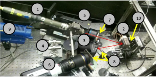
A pulsed laser (TruPulse 156, TrumpfTM, 𝜆= 1064 nm - Figure 1 (1)) is used to apply cyclic thermal shocks to the centre of a face of a parallelepiped (Figure 1 (2)). The shock frequency is 2 Hz, the pulse duration is 50 ms and the incident pulsed power is equal to 300 W. A focusing optics allows a top-hat power density to be obtained over a 5-mm disk at a working distance of 29 cm. Due to a relatively low absorptivity of the polished surface an inclination of the beam is needed to reflect the incident beam onto a calorimeter (Figure 1 (3)). The latter gives access to the mean power reflected by the sample.
One fast pyrometer (KGA740-LO , KleiberTM, 𝜆 = [1550 nm-2200 nm], Figure 1 (4)) is used to measure the temperature variations on a disk, 2.5-mm in diameter, targeted on the impacted zone, at a frequency of about 1.4 kHz. In order to have access to the average emissivity of the impacted zone, another fast pyrometer (same device) focuses on a zone of the specimen surface, outside of the impacted zone and covered by a highly emissive black painting (the procedure is explained in Section 3.3.1). Last, an infrared camera (x6540sc FLIRTM, definition: 640 × 512 pixels, 𝜆 = [3 µm-5 µm] reduced to 𝜆 = [3.97 µm-4.01 µm] with an internal filter for high temperature measurements, Figure 1 (5)) is used to measure the changes of the thermal field during the laser shocks.
A visible camera (MIRO M320S, Vision ResearchTM, definition:
1920 × 1080 pixels, Figure 1 (6)) is used to acquire pictures to measure the displacement fields via DIC. Protective filters are used for both IR and visible cameras (Figure 1 (7 and 8)). A 250-W DedocoolTM spotlight is used to provide the lighting
cameras are 18 cm and 25 cm, respectively. This leads to physical pixel sizes equal to 60 µm and 10 µm, for IR and visible cameras, respectively. The sample is heated up to 400 °C with an electrical resistance the temperature of which is controlled by a thermocouple (Figure 1 (10)).
Figure 1: Experimental configuration (see main text for a detailed description of the components labelled in the picture)
2.2. Characterized sample
The studied sample is a 50 50 10 mm3 parallelepiped made of 304L
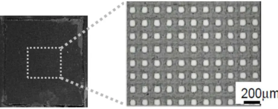
austenitic stainless steel. To measure displacement fields via DIC, a regular grid is laser-engraved onto an initially polished surface of the sample (Figure 2). The depth of the material affected by the engraving has been estimated to be 4 µm at the most (Figure 2). The resulting global emissivity is determined in different ways detailed in Section 3.3.1.
Figure 2: Regular grid laser engraved onto the surface (left), and a zoom on the pattern (right)
3. Digital Image Correlation and infrared techniques
3.1. Stroboscopic reconstruction
To measure the displacement and thermal fields at the same time, a stroboscopic acquisition is performed to compensate for the relatively low acquisition frequency of the IR camera compared with the laser shock parameters. The visible camera can acquire frames at a much higher rate than the IR camera. Yet, both cameras have been synchronized on the same signal to facilitate the comparison between simulated and experimental fields, in terms of temperature and displacement.
A LabviewTM code is developed for this purpose. It triggers not only each laser
pulse at a constant rate but also the start of any sequence of camera acquisition so that it corresponds to the emission of a new laser pulse. Based on the parameters of the laser pulse (i.e., frequency and duration) and on the maximum value of the acquisition frequency of the IR camera, the program generates a synchronized TTL signal to control the acquisition frequency of both cameras at a value that allows a unique (virtual) cycle to be reconstructed with N real successive cycles. The frequency of the signal and the number of cycles to reconstruct the virtual cycle are automatically determined by the program depending on the number of images the user wants for one laser pulse (increase of temperature).
For instance, let us consider cyclic laser shocks at a frequency of 2 Hz and pulse duration of 50ms. If the maximum acquisition frequency of the cameras is set to 180 Hz and the number of images during one pulse equals 36, then four successive thermal shocks with an effective frequency acquisition of 179.5 Hz will have to be recorded to get a complete history by stroboscopic reconstruction. This approach provides 36 pictures during one reconstructed pulse (increase of temperature only) to be compared with only 9 pictures per pulse if no stroboscopic reconstruction were used. During one complete cycle, namely, the increase of temperature and the cooling down phase, the total number of images is 359 (90 images for the first three real cycles and 89 for the fourth and last one of the stroboscopic sequence). The next image would be acquired exactly at the beginning of the fifth cycle. To reach a steady state temperature regime from one pulse to another, approximately 50 cycles are performed prior to starting the stroboscopic acquisition. The steady state character was validated with the pyrometer signals acquired continuously at a frequency of 1436 Hz during one hundred cycles.
3.2. Digital Image Correlation
The principle of DIC is to register two images shot at different instants of time, in the present case the reference image 𝑓 is shot just before the first measured shock and the deformed images 𝑔 are those acquired during the thermal loading. Most of the time, the main assumption is based upon a grey level conservation between the registered images
𝑔(𝑥 + 𝑢(𝑥)) = 𝑓(𝑥) (1)
where 𝑢(𝑥) is the sought displacement field, and 𝑥 the position of any pixel. This conservation equation implies that the two states of the observed surface should be
illuminated with the same amount of light. In the global DIC approach used herein, the aim is to minimize the following functional over the whole region of interest
𝜏𝐷𝐼𝐶2 = ∫ (𝑓(𝑥) − 𝑔( 𝑥 + 𝑢(𝑥)))2𝑑𝑥 (2)
by iteratively correcting the deformed image as 𝑔𝑛(𝑥) = 𝑔( 𝑥 + 𝑢𝑛(𝑥)) until convergence. The convergence criterion is given by the root mean square (RMS) difference between the displacement at iteration 𝑛 + 1 and 𝑛, which has to become less than 10-6 pixel. The correlation residual field is the final grey level difference (𝑓(𝑥) − 𝑔𝑛(𝑥)) whose quadratic norm is the minimized cost function 𝜏
𝐷𝐼𝐶2 . In the following
regularized FE-DIC is used. The principle consists of discretizing the displacement
field with finite elements so that the kinematic unknowns become the nodal displacements [10]. In the present case, 3-noded triangular (T3) elements are chosen. Instead of directly minimizing Eq. (2), the minimization is performed on the total functional 𝜏𝑡, which consists of the weighted sum of three functionals, namely, one contribution based on grey level conservation, another one based on the minimization of the equilibrium gap 𝜏𝑀, and a last one controlling the displacement fluctuations on the
edges of the region of interest 𝜏𝐵
(1 + 𝜔𝑀+ 𝜔𝐵)𝜏𝑡 = 𝜏𝐷𝐼𝐶+ 𝜔𝑀 𝜏𝑀 + 𝜔𝐵 𝜏𝐵 (3)
where the weights 𝜔𝑀 and 𝜔𝐵 are proportional to the fourth power of cut-off wavelengths 𝜌 of low-pass mechanical filters [11]. In the following analyses, 10-pixel T3 elements are appropriate for the displacement amplitudes to be measured and with the size of the grid pattern. Regularization lengths of 𝜌 = 200 pixels for the mechanical and boundary functionals are selected.
3.3. Infrared techniques
Non-contact temperature measurements are performed using IR pyrometers and an IR camera. First, a calibration is performed, which consists of identifying the transfer function that links the output signal of the device to the temperature of a blackbody (BB). Second, an accurate determination of the specimen emissivity is needed to transform the measured signal outputs (Digital Levels) into absolute temperatures.
3.3.1. Emissivity determination
A first approach to determine the emissivity consists of using a BB (HGH, DCN1000H4) with a large square emissive surface (100mm × 100mm) reflected by the sample surface. The Digital Level (DL) given by the IR camera is computed as [7]
𝐷𝐿 = 𝜉𝐷𝐿(𝑇𝑆) + (1 − 𝜉)𝐷𝐿(𝑇𝐵𝐵) (4)
where 𝑇𝑆 is the temperature of the sample, 𝑇𝐵𝐵 the temperature of the BB, and 𝜉 the emissivity of the specimen. In order to limit possible ambiguities, let us stress that the notation has been chosen for strains in this paper. Several temperatures of the BB are prescribed, ranging from 5 °C to 150 °C, while the temperature of the sample is unchanged. From at least two temperature levels (𝑒. 𝑔. 𝑇𝐵𝐵1 = 80 °𝐶 𝑎𝑛𝑑 𝑇𝐵𝐵2 = 100 °𝐶), the global emissivity becomes
𝜉 = 1 − 𝐷𝐿1− 𝐷𝐿2 𝐷𝐿(𝑇𝐵𝐵1) − 𝐷𝐿(𝑇𝐵𝐵2)
(5)
To further increase the sensitivity of the method, more than two values of the BB temperature may be considered. This methodology has been applied to determine the emissivity of the sample at room temperature. In that case, no internal filter is put in front of the IR sensor of the camera, thereby resulting in an absorption bandwidth of
[3 µm-5 µm].
However, in the thermal shock tests, the average temperature of the sample, which is controlled by a thermocouple, is maintained to about 400°C and thus the measurement of surface emissivity should be performed at this temperature level rather than at room temperature. Moreover, the use of a high temperature internal filter reduces the absorption bandwidth of the camera to [3.97 µm-4.01 µm], a reduction that can affect the value of global emissivity.
When the temperature of the sample is much higher than the maximum temperature admissible by the large emissive surface BB (i.e., 150 °C), the previous approach is no longer applicable. The effect of the environment (see Eq. (4)) is reduced since most of the radiative flux now comes from the heated sample, even for moderately low values of emissivity. An alternative route consists of depositing a highly emissive black coating onto one part of the sample surface near the region of interest. Then by keeping the sample at a known temperature the surface emissivity is estimated as
𝜉 =𝐷𝐿𝑅𝑒𝑔𝑖𝑜𝑛 𝑜𝑓 𝑖𝑛𝑡𝑒𝑟𝑒𝑠𝑡− 𝐷𝐿𝑂𝑓𝑓𝑠𝑒𝑡 𝐷𝐿𝐵𝑙𝑎𝑐𝑘 𝑝𝑎𝑖𝑛𝑡𝑖𝑛𝑔− 𝐷𝐿𝑂𝑓𝑓𝑠𝑒𝑡
(6)
where 𝐷𝐿𝑂𝑓𝑓𝑠𝑒𝑡 is the digital level representative of the camera noise (obtained with a BB at low temperature or the camera lens cap).
The last methodology that assesses the luminance of a region (outside the impacted zone) of the sample covered by a black paint as a reference is also used with the pyrometers to identify the emissivity in their respective spectral range [1.55 -2.2 µm]. The measurements are performed once the sample reaches a homogenous surface temperature; the later point is verified by comparing the temperatures of different coated parts surrounding the zone of interest. The laser and calorimeter also
provide the absorptivity of the surface at the laser wavelength (by subtracting the reflected energy measured by the calorimeter from the incident pulse energy).
3.3.2. Calibration phases
When IR techniques are to be used, calibration phases with BBs are important to relate the signal outputs of the measuring systems and the sought temperatures. Due to technical limitations, temperatures greater than 150 °C are calibrated with a cavity BB (instead of the previous large emissive surface BB)1. The calibration function used for the large-band pyrometer has the general form of Planck’s law, 𝑈 = 𝐴/(exp(𝐵/ 𝑇𝐵𝐵) − 1), where 𝑈 is the output voltage of the pyrometers. The calibration then consists of identifying the parameters 𝐴 and 𝐵 so that the difference between experimental and predicted output voltages be minimum for 10 values of the BB temperature ranging from 200 °C to 700 °C by steps of 50 °C.
The IR camera was provided with calibration files. However, as the manufacturer performed the calibration at a different working distance (i.e., 2 m away from the BB) and settings (no external germanium protective filter) an in-house calibration with the same settings (working distance and germanium filter) as in the experiments has been conducted. It appeared that the reduction of working distance (to 18 cm) was compensated by the introduction of the germanium window resulting in the same outputs as those proposed by the manufacturer.
1
As previously explained, even if it would have been interesting to use a high temperature BB in reflection of the IR camera with respect to the normal of the sample to determine the surface emissivity of the sample, such a cavity BB is a priori not adequate due to the presence of diffuse reflections on this surface.
4. Finite Element model and identification of parameters
To calibrate the complete experimental setup, starting from the estimation of the surface emissivity up to the displacement fields, FE simulations are carried out. These simulations also allow 3D data to be obtained, which are not directly accessible experimentally. Since the experimental temperature field is first assumed to be symmetric (Figure 3(a)), the latter is averaged as shown in Figure 3(b). This assumption is made in order to lower the computation time for the identification process. The meshing strategy used is similar to the procedure proposed in Ref. [9], namely, a fine mesh is used in the zone of impact (element size comparable to the IR pixel size of 60µm) and a coarser mesh away from the surface impacted by the laser beam. A heat transfer simulation is first performed in order to obtain the time history of the complete 3D thermal field. This temperature history is then used as an input to a thermomechanical simulation that gives access to the stress and strain fields.
The fluctuations observed in the experimental temperature profiles of Figure 3(a) are the signature of the engraved surface. Such fluctuations could be reduced by considering an emissivity field (pixel to pixel emissivity determination) rather than using an averaged emissivity. However, since experimental data are subjected to significant levels of noise, the change of temperature at a single pixel level is not considered. Instead, the long-distance spatial changes of the temperature field are sought at a given time or alternatively the temporal history of the temperature averaged over an area containing at least 10 pixels. At this scale, there is no need for more complexity than an average emissivity between the two local emissivity values of the edges and centre of the engraved parts. The FE simulations will thus only have to match at best an average of the temperature profile reported in Figure 3(a). It will also be shown that using the symmetry assumption and the averaged quarter IR frame reduces these fluctuations (see Figure 6).
(a) (b)
Figure 3: (a) Profiles along Y and Z axes for a row of pixels corresponding to (b) the measured temperature field at the end of a laser shock
A representation of the symmetric assumptions, the 3D geometry of the numerical model, the boundary conditions of the heat transfer simulation and the resulting thermal field at the end of a laser pulse are shown in Figure 4. The three planar free surfaces (X = 0, Y = YMax and Z = ZMax) are assumed to undergo free convection
with a coefficient of 25 𝑊 ∙ 𝑚−2∙ 𝐾−1. The influence of this parameter has been found
to be rather weak on the results presented hereafter and it is set to this nominal value in the identification process. On the rear surface of the sample (X = XMax), a constant
temperature is prescribed (i.e., T = 383 °C) corresponding to the experimental boundary conditions of the electrical resistance (Figure 1). The value of this prescribed temperature is also imposed on the complete 3D mesh at the beginning of the heat transfer simulation.
Figure 4: Illustration of the symmetric thermal boundary conditions (with the identified super-Gaussian) applied to the 3D model. The dotted box represents the zone of finer
mesh.
A top-hat heat flux is prescribed on the central zone of the surface in contact with the laser beam. The laser should ideally illuminate uniformly a region that is an ellipse, of semi-axes 𝑅𝑦 and 𝑅𝑧 along the horizontal and vertical directions, 𝑦 and 𝑧, respectively. Introducing the reduced distance 𝑟(𝑦, 𝑧)2
𝑟(𝑦, 𝑧)2 = (𝑦 𝑅𝑦) 2 + (𝑧 𝑅𝑧) 2 (7)
the boundary condition for a top-hat power density I is written as
𝐼(𝑧, 𝑦) = 𝐴𝜆𝑙𝑎𝑠𝑒𝑟𝐼0H(1 − 𝑟(𝑦, 𝑧)) (8)
where 𝐼0 is the applied laser power, and H the Heaviside function. Three parameters are identified in this analysis, namely, the radii of the “top-hat” shape 𝑅𝑦 and 𝑅𝑧, and the
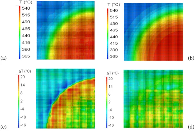
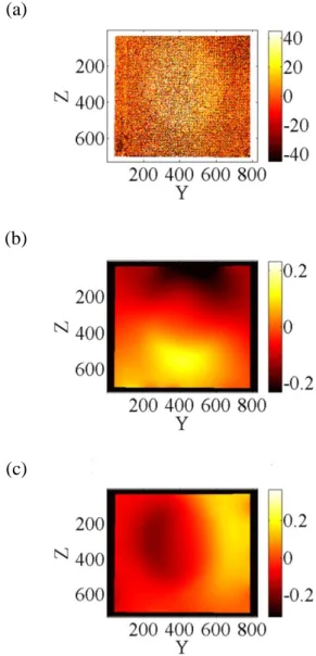
absorption coefficient of the surface 𝐴𝜆𝑙𝑎𝑠𝑒𝑟 at the laser wavelength. All remaining material parameters are taken from the French design code for nuclear power plants [12]. The Levenberg-Marquardt procedure of Sidolo software [13] is then used to identify the set of parameters that minimizes the difference between the simulated (Figure 5(b)) and measured (Figure 5(a)) temperature fields at the end of a laser pulse. In order to reach a steady state cyclic regime in the simulations, at least four successive cycles must be run. Therefore, in the identification process, the experimental data are compared with the numerical results of the last of six successive cycles. The final difference is plotted in Figure 5(c). The residual map is nearly uniform in some regions and presents very low values. However a ring of higher amplitudes is observed, which is interpreted by the fact that the experimental shape of the laser beam is not a perfect top-hat. The absorbed power density can be better described by a super-Gaussian [14] function 𝐼(𝑧, 𝑦) = 𝐴𝜆𝑙𝑎𝑠𝑒𝑟𝐼0 𝑝 4 1 𝑝 2𝜋Γ (2𝑝)𝑒𝑥𝑝(−2𝑟(𝑧, 𝑦) 𝑝) (9)
where Γ is the gamma function and p is an additional parameter to be identified. It is worth noting that if the power p equals 2, a Gaussian profile is obtained. Similarly, if the power p tends to infinity (𝑝 → ∞) a top-hat is recovered [14]. The new identification of the thermal loading with such profile leads to an intermediate value, namely, 𝑝 = 11. The resulting residual map is then clearly lowered (Figure 5(d)). The observed ring in Figure 5(c) disappears and the RMS residual decreases from 2.1 to 1.2 °C. In the following simulations, the super-Gaussian profile will be considered.
(a) (b)
(c) (d)
Figure 5: (a) Projection of the averaged experimental temperature field on the finite element mesh and (b) corresponding simulated field after the identification of the parameters of the super-Gaussian power density function. Residual maps representing
the difference between the identified and experimental temperature fields (°C) with a top-hat (c) and super Gaussian (d) functions
Once all parameters of the thermal model are identified, thermomechanical simulations are performed in which the history of the temperature field in the sixth cycle of the previous thermal simulation is prescribed as an input. Six thermomechanical cycles with the same thermal loading are found to be sufficient to reach a stabilization of the mechanical response of the material. This mechanical behaviour is described by a nonlinear kinematic hardening law identified on the results of push-pull fatigue tests carried out at 165 °C and 320 °C [15]. This law has already been used to estimate the strain variations in other thermal fatigue experiments [9] and is briefly summarized hereafter.
The total strain tensor𝜺is expressed as
𝜺 = 𝜺𝑀+ 𝜺θ (10.1)
with the thermal strain tensor, and M the mechanical strain tensor
𝜺𝑀 = 𝜺𝑒+ 𝜺𝑝 (10.2)
where e is the elastic strain tensor (describing isotropic elasticity). The relationship between the stress tensor and the plastic strain tensor p reads
𝜺̇𝑝 = 𝜆 ̇𝜕𝑓
𝜕𝝈 (10.3)
where 𝜆 ̇ is the plastic multiplier. The yield function 𝑓 is defined by
𝑓 = 𝐽2(𝝈 − 𝑿) − 𝜎𝑌 ≤ 0 (10.4)
with J2 the second invariant of deviatoric tensors, 𝜎𝑌 the yield stress and X the
back-stress tensor
𝑿 ̇ = 𝑏 (2
3𝑔𝜺̇𝑝− 𝑿𝑝̇) (10.5)
𝑝̇ = √(2
3𝜺̇𝑝: 𝜺̇𝑝) (10.6)
Only the Young modulus, Poisson ratio, yield stress and the two hardening coefficients
b and g are needed. The thermomechanical properties are listed in Table 1 [15], [16].
Table 1: Thermophysical properties. T is the temperature expressed in °C
Parameter Value Unit
Density −0.44𝑇 + 7980 kg/m3
Thermal expansion
coefficient 0.008𝑇 + 16.43 10-6 K-1
Specific heat 0.2𝑇 + 465 J/kg.K
Thermal conductivity 0.014𝑇 + 13.6 W/m.K
Young’s modulus −0.082𝑇 + 194 GPa
Yield stress 102 MPa
Hardening parameter g 114 MPa
Hardening parameter b 532 _
Poisson’s ratio 0.3 _
5. Results and discussions
5.1. Experimental and identified thermal loading
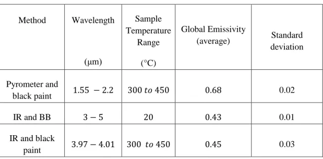
Table 2 shows the results obtained by the different approaches presented in Section 3.3.1 to determine the surface emissivity of the sample. The reported standard deviations are resulting from 5 successive measurements. As expected, the emissivity varies with the wavelength [17]. It is noteworthy that there is no change in surface emissivity (or absorptivity) when the values before and after laser shocks are compared.
It is concluded that the same amount of flux is absorbed by the sample during all cyclic laser pulses and thus that a constant loading is applied (it was independently checked, using dedicated experiments, that the laser source did not drift). According to theoretical and experimental predictions [17]-[18] the emissivity for metals should increase with the temperature. It can be noticed that the estimated emissivity for the IR camera increases by 4 % from ambient to higher temperatures (300-400 °C). This increase may result from either an increase of metal surface emissivity with temperature or the considered wavelength ranges, which are reduced for higher temperatures due to the filter. It can also be due to other sources such as measurement uncertainties. Referring to the standard deviation there is an uncertainty of 0.03 between successive measurements, which can explain such gap. It has to be emphasized (see Figure 2 (b)), that the surface of the sample has two specific features, namely, roughness and partial oxidation, due to engravings. According to Ref. [19], the emissivity of rough and/or oxidized metallic surfaces decreases with the temperature. Hence by considering the combination of opposite trends, namely, an increase of emissivity with temperature for metallic surfaces and a decrease of emissivity for rough and/or oxidized surfaces can explain why the estimated emissivities are nearly constant with temperature. Consequently, it is assumed that the emissivity does not evolve with temperature. An error assessment accounting for emissivity uncertainty is proposed in the sequel.
Table 2: Emissivity and absorptivity results Method Wavelength (μm) Sample Temperature Range (°C) Global Emissivity (average) Standard deviation Pyrometer and black paint 1.55 − 2.2 300 𝑡𝑜 450 0.68 0.02 IR and BB 3 − 5 20 0.43 0.01 IR and black paint 3.97 − 4.01 300 𝑡𝑜 450 0.45 0.03
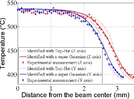
The identification step provides results that are very close to the experimental observations when the absorptivity (0.34 at 540 °C) determined via FE simulations is compared with the experimental level (0.35 at 300 °C) at the laser wavelength. The size of the hot zone is well approached by both types of power density functions (i.e., top-hat and super Gaussian) since the temperature profiles along both axes are comparable to the experimental ones (Figure 6). The super Gaussian profile power was identified to be 𝑝 = 11. As discussed in Section 4, the residual errors are lower (see Figure 5 (c-d)) with the latter. The profiles shown in Figure 6 also confirm this result. The identified absorptivity coefficient is equal in both cases to 0.34. Using a top-hat profile leads to radii of 2.5 cm along Y and 2.8 cm along Z, whereas the super-Gaussian profile (with 𝑝 = 11) provides radii equal to 2.8 cm and 3.1 cm along Y and Z axes, respectively.
Figure 6: Averaged experimentally measured (IR) and identified temperature profiles along the vertical (Z, red) and horizontal directions (Y, blue) at the end of a laser shock.
The dashed line corresponds to the prediction with a top-hat power density function, and the solid line with a super-Gaussian
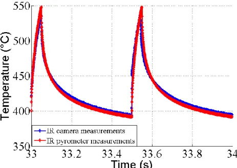
The temperature measured by one pyrometer is then compared in Figure 7 with that obtained with the IR camera. This last measurement is the result of a spatial average over 10 pixels located in the center of the zone impacted by the laser. These last results are similar with a gap of 10 °C at the most (e.g., the pyrometers indicate 550 °C while the IR camera 540 °C as maximum temperatures). No change in emissivity has been noted in the range 20 °C to 400 °C, and hence no significant variation is expected when the temperature increases up to 550 °C. Therefore, the high speed pyrometer and IR camera are expected to be reliable for the present experimental conditions.
Figure 7: Temperature history in the centre of the laser beam measured by the large-band pyrometers and IR thermography
A simple error assessment is now proposed on the thermal loading measurements. The temperature measurement error is related to the error in emissivity [20] for monochromatic detectors
∆𝑇 = 𝜆 Δ𝜉 𝜉𝑐2 𝑇2
(11)
with T the absolute temperature (expressed in K), 𝜉 the emissivity at wavelength 𝜆 and 𝑐2 a constant equal to 1.4388 ∙ 10−2𝑚 ∙ 𝐾. In the emissivity determination procedure
using the black paint, it is assumed that the emissivity of the coated part equals 1. Assuming that this parameter is overestimated by 7.5% (i.e., the emissivity is equal to 0.92 instead of 1), the errors on the temperature determination of a sample for which the real temperature is 400 °C are equal to 9 °C and 5 °C at the IR camera and pyrometer working wavelengths respectively. Therefore the error on the emissivity determination
of the impacted zone at 400 °C could be of the order of 6.2 % and 8.2 % at the IR camera and pyrometer wavelengths respectively. Considering such levels of error on the emissivity determination, it is now possible to estimate the error in the temperature measurements during the laser shocks (assuming the emissivity is independent of the temperature). The measurement errors are equal to 12 °C and 5 °C at 550 °C and 11 °C and 8 °C at 400 °C for the IR camera and high speed pyrometer respectively.
This error analysis shows how sensitive the IR measuring tools are to the surface emissivity determination. By introducing an error on the black paint emissivity of 7.5 %, the error of the measured temperature at 550 °C at the IR camera wavelength is equal to 12 °C. A good practice would then be to add in some part of the sample thermocouples (far enough from the impacted zone). This would allow the measured temperatures by the radiative and contact methods to be compared. Another way to reduce the errors is to use a black paint of known emissivity [21].
5.2. Kinematic fields
As the displacement fields are expected to be small along the Z and Y directions, it is necessary to assist DIC calculations by using a regularized approach. The T3-mesh size is 10 pixels. Different regularization lengths have been tested, from 𝜌 = 50 to 200 pixels. The displacement fields are similar but the spatial fluctuations induced by measurement noise are increasing while 𝜌 is decreasing. For instance the RMS value between the fields along Z, for 𝜌 = 50 and 𝜌 = 200 pixels is equal to 8 ∙ 10−3 pixel. The derived strains are more easily interpretable and comparable to FE
predictions when a large regularization length is used. Hence the selected regularization parameter is 𝜌 = 200 pixels. The residual errors are small compared with the image dynamic range (since a 12-bit digitization is used, see Figure 8(a)), namely, the RMS grey level is equal to 0.6 % of the dynamic range. However, the maximum residuals
correspond to the signature of the laser beam. This is due to the fact that the visible camera is sensitive to the flux in the near IR wavelength even behind two protective hot mirrors. Hence the grey levels are not totally conserved. This effect is only observed on deformed images shot when the laser is on (i.e., not upon cooling down). However, it is believed to have minimal influence on the displacement field measurement as the regularization has been activated.
(a)
(b)
(c)
Figure 8: (a) Correlation residual map expressed in grey levels (dynamic range of the picture: 4080 grey levels). Displacement fields along Y (b) and Z (c) axes (expressed in pixel) between pictures taken just before starting a laser pulse and at the end of the laser
The measured displacement fields correspond to a ‘biaxial’ tensile test (Figure 8(b and c)), in the sense that displacement gradients are observed in both directions. The displacement amplitudes (expressed in pixels) are rather small during thermal loading. The maxima reached along the Y and Z axes are about 0.2 pixel, which is equivalent to 2 µm. There is a zone where the displacements are equal to zero close to the centre of the zone impacted by the laser beam. In-plane strains are then calculated from the measured displacement fields. An FE-DIC calculation has been run using two images of the reference configuration (i.e., first two images before the laser shock). This allows the measurement resolution to be determined. The RMS values of the displacement fields (along Z and Y) are equal to 7 ∙ 10−3 pixel. The corresponding standard strain uncertainties are of the order of 3 ∙ 10−5.
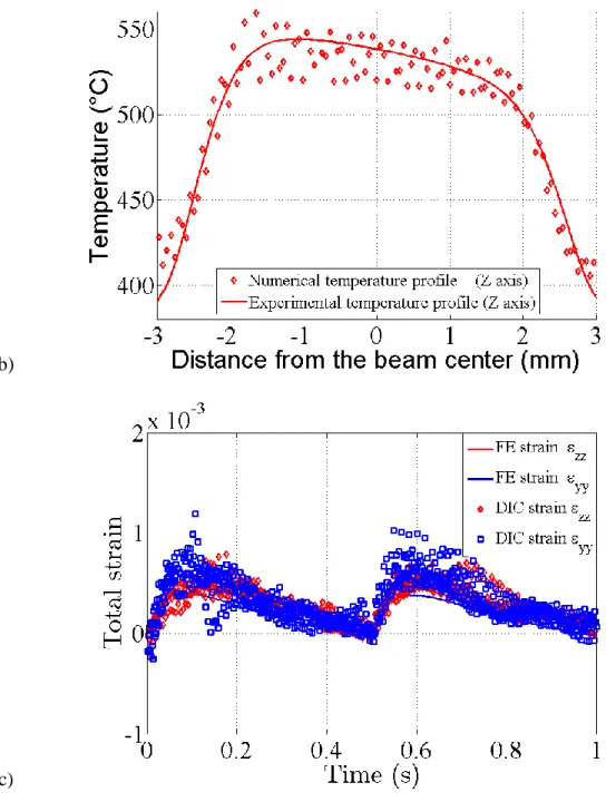
The comparison between the experimental levels with the FE results focuses on the total strain components, which result from thermal expansion and mechanical stresses induced by temperature gradients. The DIC results (Figure 9(a)) show that the profile of vertical strains 𝜀zz is not symmetric along the Z direction as opposed to that of
the horizontal strains 𝜀yy. This presumably results from the fact that the temperature
profile along the Z axis is not perfectly symmetric (Figure 3(a)).
The DIC measurements and the FE results lead to similar spatiotemporal responses (Figure 9). The dissymmetric mechanical response can be explained by the prescribed thermal loading. By referring to Figure 9(b) where the experimental profiles are plotted, it is observed that along the Z axis the symmetry hypothesis is not satisfied. The simulations have thus been run with a super-Gaussian profile and symmetry relaxations along the Z axis, see Figure 9 (b). The prescribed heat flux then reads
𝐼𝐷(𝑦, 𝑧) = I(y, z) (1 − 𝑎𝑧
2𝑅𝑧) (12)
where 𝑎 is also a parameter to be identified. It is worth noting that the power density satisfies the global power conservation
∬+∞𝐼𝐷(𝑦, 𝑧) 𝑑𝑦𝑑𝑧
−∞ = ∬ 𝐼(𝑦, 𝑧) 𝑑𝑦𝑑𝑧
+∞
−∞ = 𝐴𝜆𝑙𝑎𝑠𝑒𝑟𝐼0 (13)
Using the last approach allows the thermal loading to be closer to the experimental temperature field and the same 𝜀𝑧𝑧 profile to be found. The measured strain levels are in
good agreement with the calculated ones. For instance, the total strain 𝜀𝑦𝑦 at the end of the thermal (50-ms) shock in the center of the beam is equal to 5 ∙ 10−4 with DIC whereas the FE simulations predict a level of 4 ∙ 10−4. The measured and predicted strains 𝜀𝑧𝑧 are well superimposed even if some small gaps remain (Figure 9(a)). It is worth noting that the standard strain resolutions are 3 ∙ 10−5 for 𝜀𝑧𝑧 and 2 ∙ 10−5 for 𝜀𝑦𝑦.
Even though Figure 9(a) shows a good agreement between the measured and simulated levels at the instant of maximum temperature reached during the thermal shock, care must be exercised when drawing conclusions concerning the good match of experimental and numerical results over the whole history of one laser pulse. The temporal changes of the eigen strains extracted at the beam axis are plotted in Figure 9c. Significant fluctuations are observed on this signal. They are not really surprising considering, on the one hand, the low level of displacement amplitudes measured at the end of a laser pulse, and, on the other hand, the relatively high level of noise introduced in the pictures. In other words, the DIC resolution is not significantly lower than the signal to be measured and without the spatial regularization the spatial profile of the eigen strains (Figure 9a) would be completely erratic.
These temporal fluctuations can also be due to small convection effects that distort the images. They appear not only to modify the level of eigen strains on the beam axis from one picture to another, they also modify their profiles leading to non-symmetric responses that can be quite different from the plotted ones in Figure 9a. This last point is not yet fully understood.
Different calibration procedures have been performed with the visible camera to improve DIC measurements such as taking into account lens distortions [22] and parallax effects due to the inclination of the camera with respect to the normal of the surface sample. The new results yielded no significant improvements compared with those presented above. Spatiotemporal regularization [23] is currently under investigation to further reduce the fluctuations.
(b)
(c)
Figure 9: Comparison between FE and experimental results for (a) the total eigen strain profiles at the end of the shock (50 ms) (b) the non-symmetric temperature profile along the Z direction (c) the temporal history of the eigen strains in the centre of the impacted
zone (stroboscopic reconstruction for DIC)
In spite of these shortcomings, the FE analyses also provide out-of-plane strains that are not accessible via DIC. Figure 10 illustrates for instance the fact that the level of
the total out-of-plane strain 𝜀𝑥𝑥 is much higher than the computed (or measured) strains along the Y and Z directions.
Figure 10: Predicted contributions of the thermal and mechanical parts to the in-plane and out-of-plane normal strains
This is due to the fact that along the Y and Z axes the positive thermal strains are compensated by compressive elastoplastic strains (i.e., negative mechanical strains) along the same directions (Figure 10). In the X direction, since no stresses are present in the vicinity of the free surface, both thermal and mechanical strains are positive. The out-of-plane motions are estimated to be at most 10 µ𝑚. According to Ref. [24], the overestimation of in-plane strains due to out-of-plane displacements is assessed by calculating the ratio between the out-of-plane displacement amplitude and the working distance (25 cm). In the present case the out-of-plane displacement induce an overestimation of the in-plane strain component of about 4 ∙ 10−5, which is very close
6. Summary
A new experimental setup using laser shocks has been presented to study thermal fatigue of austenitic stainless steels. Experimental techniques providing both thermal and kinematic fields within the loaded region have been proposed. Temperature measurements are performed with an IR camera and pyrometers. The results given by both methods are very close. As these methods require the determination of the surface emissivity, different procedures provide the needed estimates at relevant wavelength ranges.
Once the temperature field is estimated, an identification of the parameters of the laser beam is carried out by minimizing the difference between the thermal fields obtained experimentally and by FE analyses at the end of a laser pulse. Parameters such as the absorptivity of the surface are very close to experimental values. This identification step is needed to assess the thermal loading of the analysed experiment. A super-Gaussian beam shape appears to reproduce very accurately the spatial power density of the laser (better than a mere top-hat).
The measured eigen strains are compared with the predicted levels based on an elastoplastic simulation. The asymmetry of the total strain profile 𝜀𝑧𝑧 is explained by the asymmetry of the thermal loading in the same direction. The measured and predicted strain levels have similar profiles and amplitudes at a specific time (maximum of the thermal loading). However the temporal comparisons between the experimental measurements and FE results are prone to fluctuations. This last point will require additional investigations.
Last, thermal fatigue experiments will be carried out in which the in-situ thermal and kinematic fields can be measured with the proposed setup. It will then be possible to compare thermal and mechanical fatigue properties of various materials.
References
[1] F. Curtit, “INTHERPOL thermal fatigue test,” Proceedings of the third international conference on fatigue of reactor components, Seville, Spain, Oct-2004.
[2] V. Maillot, A. Fissolo, G. Degallaix, and S. Degallaix, “Thermal fatigue crack networks parameters and stability: an experimental study,” Micromechanics
Mater., vol. 42, no. 2, pp. 759–769, Jan. 2005.
[3] N. Kawasaki, S. Kobayashi, S. Hasebe, and N. Kasahara, “SPECTRA Thermal Fatigue Tests Under Frequency Controlled Fluid Temperature Variation: Transient Temperature Measurement Tests,” presented at the ASME 2006 Pressure Vessels and Piping/ICPVT-11 Conference, Vancouver, BC, Canada, 2006, vol. Volume 3: Design and Analysis.
[4] O. Ancelet, S. Chapuliot, G. Henaff, and S. Marie, “Development of a test for the analysis of the harmfulness of a 3D thermal fatigue loading in tubes,” Int. J.
Fatigue, vol. 29, no. 3, pp. 549–564, Mar. 2007.
[5] A. Fissolo, S. Amiable, O. Ancelet, F. Mermaz, J. M. Stelmaszyk, A. Constantinescu, C. Robertson, L. Vincent, V. Maillot, and F. Bouchet, “Crack initiation under thermal fatigue: An overview of CEA experience. Part I: Thermal fatigue appears to be more damaging than uniaxial isothermal fatigue,” Int. J.
Fatigue, vol. 31, no. 3, pp. 587–600, Mar. 2009.
[6] A. Fissolo, C. Gourdin, O. Ancelet, S. Amiable, A. Demassieux, S. Chapuliot, N. Haddar, F. Mermaz, J. M. Stelmaszyk, A. Constantinescu, L. Vincent, and V. Maillot, “Crack initiation under thermal fatigue: An overview of CEA experience: Part II (of II): Application of various criteria to biaxial thermal fatigue tests and a first proposal to improve the estimation of the thermal fatigue damage,” Int. J.
Fatigue, vol. 31, no. 7, pp. 1196–1210, Jul. 2009.
[7] L. Vincent, M. Poncelet, S. Roux, F. Hild, and D. Farcage, “Experimental Facility for High Cycle Thermal Fatigue Tests Using Laser Shocks,” Fatigue Des. 2013
Int. Conf. Proc., vol. 66, no. 0, pp. 669–675, 2013.
[8] C. Esnoul, L. Vincent, M. Poncelet, F. Hild, and S. Roux, “On the use of thermal and kinematic fields to identify strain amplitudes in cyclic laser pulses on AISI 304L strainless steel,” presented at the Photomechanics, Montpellier, 2013.
[9] A. Amiable, S. Chapuliot, S. Contentinescu, and A. Fissolo, “A computational lifetime prediction for a thermal shock experiment, Part I: Thermomechanical modeling and lifetime prediction,” Fatigue Fract. Eng. Mater. Struct., vol. 29, pp. 209–217, 2006.
[10] G. Besnard, F. Hild, and S. Roux, “‘Finite-Element’ Displacement Fields Analysis from Digital Images: Application to Portevin–Le Châtelier Bands,” Exp. Mech., vol. 46, no. 6, pp. 789–803, 2006.
[11] Z. Tomicevic, F. Hild, and S. Roux, “Mechanics-aided digital image correlation,”
J. Strain Anal. Eng. Des., vol. 48, no. 5, pp. 330–343, 2013.
[12] RCC-MX, “Règles de Conception et de Construction des Matériels Mécaniques des Ilots Nucléaires REP.” Afcen, 2005.
[13] G. Cailletaud and P. Pilvin, “Inverse Problems in Engineering,” pp. 79–86, 1994. [14] D. L. Shealy and J. A. Hoffnagle, “Laser beam shaping profiles and propagation,”
Appl. Opt., vol. 45, no. 21, pp. 5118–5131, Jul. 2006.
[15] V. Maillot, “Amorçage et propagation de réseaux de fissures de fatigue thermique dans un acier inoxydable austénitique de type X2 CrNi18-09 (AISI 304 L),”
L’école Centrale de Lille et l’Universté des Sciences et Technologies de Lille, Lille, 2003.
[16] RCC-M, “Règles de Conception et de Construction des Matériels Mécaniques des Ilots Nucléaires REP.” Afcen, 2009.
[17] G. Gaussorgues, La thermographie infrarouge, 4th ed. TEC&DOC, 1999.
[18] C. R. Roger, S. H. Yen, and K. G. Ramanathan, “Temperature variation of total hemispherical emissivity of stainless steel AISI 304,” J. Opt. Soc. Am., vol. 69, no. 10, pp. 1384–1390, Oct. 1979.
[19] C. Martin and P. Fauchais, “Mesure par thermographie infrarouge de l’émissivité de matériaux bons conducteurs de la chaleur. Influence de l’état de surface, de l’oxdation et de la température,” Rev Phys Appl Paris, vol. 15, no. 9, pp. 1469– 1478, 1980.
[20] P B Coates, “Multi-Wavelength Pyrometry,” Metrologia, vol. 17, no. 3, p. 103, 1981.
[21] M. R. Dury, T. Theocharous, N. Harrison, N. Fox, and M. Hilton, “Common black coatings – reflectance and ageing characteristics in the 0.32–14.3 μm wavelength range,” Opt. Commun., vol. 270, no. 2, pp. 262–272, Feb. 2007.
[22] J.-E. Dufour, F. Hild, and S. Roux, “Integrated digital image correlation for the evaluation and correction of optical distortions,” Opt. Lasers Eng., vol. 56, no. 0, pp. 121 – 133, 2014.
[23] G. Besnard, F. Hild, J.-M. Lagrange, P. Martinuzzi, and S. Roux, “Analysis of necking in high speed experiments by stereocorrelation,” Int. J. Impact Eng., vol. 49, no. 0, pp. 179–191, Nov. 2012.
[24] M. A. Sutton, J. H. Yan, V. Tiwari, H. W. Schreier, and J.J. Orteu, “The effect of out-of-plane motion on 2D and 3D digital image correlation measurements,” Opt.
List of figures
Figure 1: Experimental configuration (see main text for a detailed description of the components labelled in the picture) ... 5 Figure 2: Regular grid laser engraved onto the surface (left), and a zoom on the periodic pattern (right) ... 6 Figure 3: (a) Profiles along Y and Z axes for a row of pixels corresponding to (b) the measured temperature field at the end of a laser shock. ... 13 Figure 4 : Symmetric Thermal Boundary conditions on the 3-D sample and plot of the thermal field at the end of a laser pulse (with a Gaussian profile and the imposed
temperature at the rear of the surface is 365°C). ... 14 Figure 5: (a) Projection of the averaged experimental temperature field on the finite element mesh and (b) the corresponding simulation field after identification of the parameters of the super-Gaussian power density function. Residual maps representing the difference between the identified and experimental temperature fields (°C) with a top-hat (c) and super Gaussian (d) functions. ... 16 Figure 6: Averaged experimentally measured (IR) and identified temperature profiles along the vertical (Z, red) and horizontal directions (Y, blue) at the end of a laser shock. The dashed line corresponds to the prediction with a top-hat power density function, and the solid line with a super-Gaussian one. ... 21 Figure 7: Temperature history in the centre of the laser beam measured by the large-band pyrometers and IR thermography ... 22 Figure 8: (a) Correlation residual map expressed in grey levels (dynamic range of the picture: 4080 grey levels). Displacement fields along Y (b) and Z (c) axes (expressed in pixel) between a picture taken just before the start of a laser pulse and a picture captured at the end of the laser pulse. ... 24
Figure 9: Comparison between FEA and Experimental results on (a) the total eigen strain profiles at the end of the shock (50 ms) (b) the non-symmetric temperature profile along the Z direction (c) the temporal evolution of the eigen strains in the centre of the impacted zone (stroboscopic reconstruction for DIC) ... 28 Figure 10: Predicted contributions to the thermal strain and mechanical strain ... 29
List of tables
Table 1 : Thermophysical properties. T is absolute temperature in °C. ... 18 Table 2: Emissivity and absorptivity results... 20