Edge turbulence effect on ultra-fast swept reflectometry core measurements in tokamak plasmas

HAL Id: hal-02565057

https://hal.univ-lorraine.fr/hal-02565057

Submitted on 6 May 2020

HAL is a multi-disciplinary open access

archive for the deposit and dissemination of

sci-entific research documents, whether they are

pub-lished or not. The documents may come from

teaching and research institutions in France or

abroad, or from public or private research centers.

L’archive ouverte pluridisciplinaire HAL, est

destinée au dépôt et à la diffusion de documents

scientifiques de niveau recherche, publiés ou non,

émanant des établissements d’enseignement et de

recherche français ou étrangers, des laboratoires

publics ou privés.

Edge turbulence effect on ultra-fast swept reflectometry

core measurements in tokamak plasmas

G. Zadvitskiy, Stéphane Heuraux, C Lechte, S. Hacquin, R. Sabot

To cite this version:

G. Zadvitskiy, Stéphane Heuraux, C Lechte, S. Hacquin, R. Sabot. Edge turbulence effect on ultra-fast

swept reflectometry core measurements in tokamak plasmas. Plasma Physics and Controlled Fusion,

IOP Publishing, 2018, 60 (2), pp.025025. �10.1088/1361-6587/aa9807�. �hal-02565057�

Edge

turbulence effect on ultra-fast swept

re

flectometry core measurements in

tokamak

plasmas

G

V Zadvitskiy

,

S Heuraux

,

C Lechte

,

S Hacquin

and

R Sabot

1

Institut Jean Lamour UMR 7198 CNRS—Université de Lorraine, BP 70239, F-54506 Vandoeuvre-lès-Nancy, Cedex France

2 _{Institut für Grenzflächenverfahrenstechnik und Plasmatechnologie IGVP, Universität Stuttgart, Germany} 3

CEA, IRFM, F-13108 Saint-Paul-lez-Durance, France

4 _{PMU EUROfusion Culham Science Centre/K1 Abingdon Oxfordshire OX14 3DB United Kingdom}

E-mail:georgiy.zadvitskiy@univ-lorraine.fr

Received

Accepted for publication Published

Abstract: Ultra-fast frequency-swept reflectometry (UFSR) enables one to provide information about the turbulence radial wave-number spectrum and perturbation amplitude with good spatial and temporal resolutions. However, a data interpretation of USFR is quiet tricky. An iterative algorithm to solve this inverse problem was used in past works, Gerbaud (2006 Rev. Sci. Instrum. 77 10E928). For a direct solution, a fast 1D Helmholtz solver was used. Two-dimensional effects are strong and should be taken into account during data interpretation. As 2D full-wave codes are still too time consuming for systematic application, fast 2D approaches based on the Born approximation are of prime interest. Such methods gives good results in the case of small turbulence levels. However in tokamak plasmas, edge turbulence is usually very strong and can distort and broaden the probing beam Sysoeva et al (2015 Nucl. Fusion 55 033016). It was shown that this can change reflectometer phase response from the plasma core. Comparison between 2D full wave computation and the simplified Born approximation was done. The approximated method can provide a right spectral shape, but it is unable to describe a change of the spectral amplitude with an edge turbulence level. Computation for the O-mode wave with the linear density profile in the slab geometry and for realistic Tore-Supra density profile, based on the experimental data turbulence amplitude and spectrum, were performed to investigate the role of strong edge turbulence. It is shown that the spectral peak in the signal amplitude variation spectrum which rises with edge turbulence can be a signature of strong edge turbulence. Moreover, computations for misaligned receiving and emitting antennas were performed. It was found that the signal amplitude variation peak changes its position with a receiving antenna poloidal displacement.

Keywords: plasma turbulence, plasma reflectometry, sweeping frequency reflectometry, tokamak, edge turbulence, swept reflectometry

(Some figures may appear in colour only in the online journal)

1. Introduction

To identify the physical mechanism behind the turbulence which drives the transport in fusion plasma as ITER, accurate characterization of the turbulence required. One possible diagnostic to provide data is the reflectometry. Recent

progress in thisfield has been obtained with the development of ultra fast swept reflectometry (UFSR) [1]. This kind of

reflectometer was initially developed for density profile reconstruction [2], which permits the measurement of

turbu-lence wave-number spectrum (k-spectrum). This is mainly due to the fact that the sweeping time is now much shorter

than the typical turbulence time scale. The link between the phase measurements and the densityfluctuations is based on the analytical expression obtained for an ordinary wave with wave electricfield directed parallel to external magnetic field [3]. Thus, it is possible to extract the radial wave-number

spectrum from the UFSR data. However, the application of this formula is quite limited. As it gives the right result only when the turbulence level is small and when 2D effects do not play a major role. Other techniques to extract density per-turbation properties from the fluctuation of the signal phase were developed and applied to analyze experimental data[4].

These methods are based on an iterative solution of the inverse problem with the assumption that the main part of the information is coming from the cut-off layer vicinity. Usually, due to simplicity and very high speed, inside this algorithm, the direct problem is solved with a 1D Helmholtz equation solver [5]. This calculation does not take into account 2D

effects such as real beam geometry or the poloidal turbulence spectrum [6]. Instead of the 1D code, one can use an

approximate solution based on the reciprocity theorem [7].

This method can provide good accuracy in the case of the small turbulence level. However, as usual for tokamak dis-charges, strong edge turbulence can significantly change the reflectometer response [6]. When the probing beam crosses

the density perturbation region it distorts poloidal and radial wave phase fronts and suffers widening [8, 9]. However,

influence of the edge turbulence on core measurements has been little studied [10]. The aim of this paper is to analyze

edge turbulence effects on core measurements, tofind typical parameters of edge turbulence when spectrum is significantly changed, to analyze the signature of high level edge turbu-lence presence, and look on the possibility to use simplified weighting function approach. In section 2we will introduce the simplified weighting function approach. We will show results of reflectometry simulation in slab geometry for plasmas with edge turbulence in section3. The reflectometer phase fluctuation spectrum computed with IPF-FD3D code [11] will be compared with the simplified one based on the

reciprocity theorem model. In section 4 we investigate the possibility to detect coherent turbulence mode in the plasma core in the case of strong edge turbulence presence. Finally, in section5, simulations for Tore-Supra tokamak with real 2D geometry will be performed. In this part we will use exper-imental turbulence level and spectrum as-well as the density profile.

2. Weighting function method

Working with a closed-loop method requires high perfor-mance computational resources to ensure the convergence of the solution [12]. Full wave 2D codes [11, 13] are quite

demanding in term of computing resources so the use for closed-loop methods are still limited. However, in the scope of the Born approximation one can use the so called weighting function method (WG) based on the reciprocity theorem approach [7, 14, 15]. Using this method one can

calculate scattered by plasma turbulence from the incident

beam field then received by reflectometerʼs antenna. For the UFSR phase variation it is very important to compute total signal.

w = w + w

( ) ( ) ( ) ( )

I Iin Is . 1

Here, I( )w is the total signal with angular probing beam frequency ω which is composed of Iin - the unperturbed

reflected signal (computed without turbulence) and Is- the

field scattered from the turbulence received by antenna. In a tokamak, the turbulent modes are elongated along the magnetic field lines in the toroidal direction. Neglecting the toroidal curvature effects, which is often assumed in a toka-mak, computations in the 2D poloidal plane can be con-sidered. We will use the Cartesian coordinates system with the tokamak magneticfieldB0x, z is the radial direction, and

^ 

y B0 is the poloidal direction.

ò

w =

( ) ( ) ( ) ( )

Iin G za,y Ein za,y dy 2

where zais the antenna position in the radial direction, G - the

antenna pattern, and Ein is the unperturbed field of the

reflected wave. According to the weighting function method, in the case of O-mode the field scattered by the turbulence and received by the antenna can then be expressed as:

ò ò

where E₀out is an electric field of wave-guide fundamental mode propagating from the plasma normalized to power unit,

dn is the variation of the plasma density, e—the electron charge, me is the electron mass, and W is the weighting

function[15]. Similar expression for X-mode can be achieved

using general reciprocity theorem formalism [7]. As one can

see, Isis a complex number.

=

( ) ( ) ( ) ( )

W z y, E z y t E z y ti , , a , , . 4 Here, t is the time, Eiand Eaare the complex electricalfield of

emitting antenna and fictional field of the receiving antenna computed with a transposed dielectric tensor, respectively. Sources of bothfields should also be normalized to the power unit. Let us first consider the mono static antenna case with both the received and the emitted waves as plan waves. This is possible in the slab geometry with smooth plasma profile. Under such conditions we will express incident electric field in the vacuum region.

= +

w+f + +w f - +w f

∣ ∣_{E e}( ) ∣_{E e}∣ ( ) ∣_E ∣_e( ) ( )₅

i i t 0 in i kz t 1 out i kz t 2

where k is a probing beam vacuum wavenumber, Einand Eout

are incident and reflected waves. Eacan be expressed in the

same way. Under current assumptions∣Eout∣=∣Ein∣. Conse-quently, the total field will have a form of standing wave

f w f

= ( + ) ( + )

Ei sin kz k cos t 0 . In this case, weighting

function will look like:

f

= · =∣ ∣ ( ) ( )

W Ei Ea Ei2exp 2i 0. 6 The phase f₁ is defined by initial conditions. However the difference between the weighting function phase f₀ and receivedfield phase f₁is notfixed and should be taken into account when phase variation is computed. To simplify the

computation, we will use expression for the phase variation written under conditions of f₀=f₁= 0 but to compensate effects of different phases between scattered field and unperturbed field as well as beam wave-front curvature we have introduced parameter h w( )

df=atan( ( )h w I Is in) ( )7 η is a normalization coefficient which has to be computed for each density profile. For the UFSR phase response, it was found that the coefficient η is proportional to the square root of the unperturbed reflected signal amplitude received by the reflectometer antenna.

h( )w µ∣ ∣Iin1 2. ( )8 To use this method one should precompute the unperturbed field maps. This can be done analytically [14] or using full

wave codes [11, 13]. In the next sections, we will show

comparison of the phase spectrum computed with the full wave IPF-FD3D code and the simplified weighting function approach. This method is expected to give good results when the root mean square value (RMS) of density variations is below a few percents of the probing wave cut-off density. These values are typical of turbulence level in the plasma core region. On the other hand in the plasma edge region, the density perturbation level can reach values up to 15%–25% from the local density[12]. Even in the case when this edge

density perturbation layer is far from the cut-off layer posi-tion, it can lead to significant changes of the received signal[6].

3. High level edge turbulence effects

After crossing the edge turbulence region, the probing beam suffers some radial and poloidal change of the phase and widening. To investigate how the edge turbulence region affects core reflectometry measurements and to find a way to identify in which cases the edge turbulence plays a role we will study the reflectometer responses for the linear plasma density profile (see figure1) and realistic density fluctuation

spectrum and amplitude in slab geometry. Computation was performed using the ordinary mode wave. In these com-putations, the densityfluctuations are created by superimposing two different turbulence maps. First, there is background turbulence (red curve in figure 1) which is distributed

every-where in the plasma. This turbulence is homogeneous, isotropic and has a Gaussian k-spectrum with a correlation length of 3.4 cm. In our work, the correlation length is defined as spatial separation for which the turbulence auto-correlation function is equal to the half of its maximum value [16]. The

RMS amplitude of these perturbations is equal to 0.5% of the maximum swept frequency cut-off density nc. An edge

tur-bulence map with a Gaussian amplitude envelop centered in the edge region is added to the background turbulence (blue curve in figure1). The edge turbulence spectrum also has a

Gaussian shape. Its correlation length is of 1.7 cm. The cor-relation length values were chosen in agreement with the range of possible correlation lengths typically measured in Tore-Supra plasmas [16]. Turbulence maps are generated

using inverse Fourier transform of a 2D spectrum with ran-dom phase for each mode. To adjust 2D wave-number spectra of isotropic turbulence to 1D turbulence spectrum, an iterative method was used. To see the effect of the edge turbulence level, the reflectometer response was computed in 2D toroidal cross-section with the IPF-FD3D full wave code [11] for

different edge turbulence levels. In this code, the signal source does not do a frequency sweep. Instead, this many waves with different frequencies from the sweep are super-imposed on the emitting antenna. After the code reaches stationary solution, it record time-series of a received signal and separate the signal back to initial frequencies using Fourier transform. The same signal was computed with the simplified weighting function approach (presented in section 2). Here, we probe the region around R=75 cm. With a maximum frequency Fmax=26 GHz. First, we will compute a phase fluctuation spectrum. Further by spectrum we will mean modulus of the spectrum.

ò

= - á ñ

-f [ ] ( ) ( )

S R exp ikR dR 9

t

Figure 1.Radial plasma density profile (green) and turbulence level, composed of edge turbulence root mean square value (blue) and

background turbulence root mean square value(red).

wheref is a received signal phase, k is a wave-number value, á ñ...R and á ñ...t are averaging over the radial cut-off position

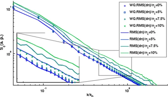
and over the time(in the case of computation, over turbulence realizations series). In figure 2, one can see the phase fluc-tuation spectrum which is specifically analyzed for turbulence k-spectrum reconstruction. Here, k0is a maximum frequency

vacuum wave-number. The spectra were averaged over 50 computations with different turbulence realizations. The number of 50 was chosen as a good compromise to extract the relevant information while keeping the computation time acceptable. We can see that the phase fluctuation spectrum carried out with the simplified weighting function approach does not change very much as long as the edge turbulence peak amplitude is below 7.5%. When the maximum of the edge turbulence reaches 10% of the cut-off density, the phasefluctuation spectrum amplitude computed with the full-wave code is more than two times higher then the same signal without edge turbulence. However, the shape of the spectrum does not change significantly and the simplified weighting function method represents it well. Here, one can see that nonlinear edge turbulence effects play a major role in the signal phase variations, and the simplified weighting function method is unable to describe these effects. This result means that assuming that the phase spectrum is connected only to the cut-off vicinity, this leads to an overestimation of the turbulence level, while it is impossible to see any sig-nature of the strong edge turbulence.

Using an USFR signal amplitude(A) analysis, it is pos-sible to extract more information about turbulence level and correlation length. For these analyses, we use a technique based on receiving the signal simultaneously in a poloidal array of antennas. Such a technique has been applied on TEXTOR and ASDEX-Upgrade tokamaks for the measure-ments of the poloidal plasma rotation and turbulence corre-lation time with a fixed frequency reflectometry diagnostic [17,18]. With this setup we can look on the average received

signal amplitude decay for the maximum swept frequency(as shown infigure3). The widening of the probing beam in that

case can be estimated from the theory [9]. Another way to

extract an information about the edge turbulence using multi-antenna configuration is to look at the UFSR signal amplitude variation spectrum.

ò

= [ - á ñ ] (- ) ( )

Sa A AR exp ikR dR . 10

t

Such spectra are illustrated in figure4. When the receiving antenna stays at the same place than the emitting one we can see a peak(figure4). This peak near =k k0is a signature of

the edge turbulence effects. When edge turbulence is absent, this peak is not observed. Following the Bragg rule

= +   

ka ki kturb, we can see that the peak close tok=k0 is

connected to enhanced scattering in the edge region. With the receiving antenna shift, we also see a shift of this peak in the direction of smaller wave-numbers. To efficiently receive the back-scattering signal with a misaligned receiving antenna, the probing beam should make a turn. As the beam propagates deeper through the strong edge turbulence layer, the probability to get stronger probing beam deviation from the edge turbulence poloidal spectrum increases. Deeper in the plasma means smaller probing wave-numbers which we see with the antenna shift. These peaks also appear in the amplitude variation spectrum when the edge turbulence reaches aRMS(dn) nc=7.5%but they are smaller and don’t move much with the receiving antenna poloidal shift.

4. Possibility to detect coherent modes in the core region in presence of strong edge turbulence To understand how the wave behavior between the cut-off and edge turbulence layers and check the possibility to detect single mode structures such as GAM[19] through strong edge

Figure 2.Phasefluctuation spectrum computed using the simplified weighting function method (spread points) and the full wave code (continuous lines), k0is a maximum frequency vacuum wave-number.

turbulence (RMS(dn) nc=10%), simulations were carried out in the same conditions than in the previous section replacing the core turbulence by a localized single mode with the same size as the edge turbulence envelope and maximum value of 0.5%. It is situated between the highest frequency

cut-off position and the edge turbulence with the center near =

n 0.75nc(see figure5). This turbulence has a single

wave-number chosen to fulfill the Bragg scattering condition ( =k 0.9k0). This mode is tilted with an arbitrary angle of 15o

with respect to the probing beam direction. Infigure6, phase

Figure 3.Averaged signal amplitude received by the receiver antenna as function of the poloidal antenna positions. A0is the emitting antenna

amplitude.

Figure 4.Signal amplitude variation spectrum at different receiver poloidal positions. The maximum RMS edge turbulence amplitude is 10% of the cut-off density.

Figure 5.RMS value amplitude envelops of edge turbulence(blue), and core turbulence (red). Maximal and minimal frequency cut-off position.

fluctuation spectra for different poloidal positions of the antenna are depicted. It shows that it is possible to detect the coherent mode through a strong turbulence layer in the edge region. To get a more smoother curve here, 100 runs with different turbulence realizations were used. It can be noticed from the equation (4) that the diagnostic is more

sensitive to core turbulence comparing to the edge turbulence with the receiving antenna shift. As receiving and emitting antennas electricfields has stronger overlap at the core region then at the edge when antennas are not aligned. The spectral peak associated with the coherent mode is double. Figure 7

shows the amplitudefluctuation spectrum for different edge turbulence amplitudes. We can see that the coherent mode is clearly observed on the spectrogram even through very high levels of turbulence. One can notice that the coherent peak in the amplitude variation spectrum is doubled as for the phase variation spectrum. First, the smallest wave-number peak

does not change much in amplitude and position with the antenna shift. Second, higher wave-number peaks decreases in amplitude and moves towards the direction of higher wave-numbers with the antenna misalignment. To analyze the nature of this peak behaviour, let us look at the complex signal spectrum:

ò

= · ( ) (- ) ( )

Ssig A exp i exp ikR dR . 11

t

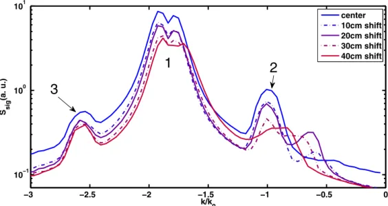
Such spectra are shown in figure 8. In the complex signal spectrum, it is possible to discriminate signals corresponding to different time of flights. In the same way that the phase time slope df w( ) dt allows to measure poloidal plasma velocity by Doppler reflectometry; here, f wd ( ) dw allows the separation of signals by the time of flight as this value grows with the time offlight. The larger the time of flight of the component of the reflected signal the smaller the

Figure 6.Signal phasefluctuation spectrum at different receiver antenna poloidal positions. The maximum RMS edge turbulence amplitude is 10% of the cut-off density.

Figure 7.Signal amplitudefluctuation spectrum computed at different receiving antenna position. The maximum RMS edge turbulence amplitude is 10% of the cut-off density.

associated wavenumber k at which it is observed in the spectrum. Infigure8, we can see a large doubled central peak (noted as 1 in figure8) and two smaller ones on both sides

(noted as 2 and 3 in figure8). The big peak corresponds to

main scattering from the cut-off region. As the coherent tur-bulence is situated between the edge turtur-bulence and the cut-off layer, it generates smaller peaks on the sides of the spectrogram. The right peak(noted as 2 in figure 8) results

from the first time the probing beam crosses the coherent turbulent layer. It is also possible to see smaller peaks from the edge turbulence as in previous section. The left peak comes from scattering after reflection by the cut-off layer. This makes us understand the nature of the two peaks observed in the amplitude and phase variation spectra. It is clear that the peak atfixed position (figure7) corresponds to

the second scattering and that the‘moving’ peak results from thefirst scattering. The peak displacement can be explained by the Bragg scattering rule. During the second scattering occurrence the probing beam has a much wider direction range. This contributes to an increase in the wave scattering efficiency and make the peak visible even when probing wave amplitude is much smaller after cut-off reflection. For the first scattering occurrence, as the turbulence wave-number isfixed, the Bragg scattering rule is satisfied for slightly higher wave-numbers. When the receiving antenna is shifted, the effective direction to receive the scattered signal changes and the scat-tering wave-number value increases. However, absence of the unique beam direction after the cut-off reflection makes the second scattering spectral peak to be stationary.

5. Reflectometry simulation in real tokamak geometry

The poloidal plasma curvature and higher density slope in the edge region can change the typical influence of the edge turbulence on core radial wave-number measurements using

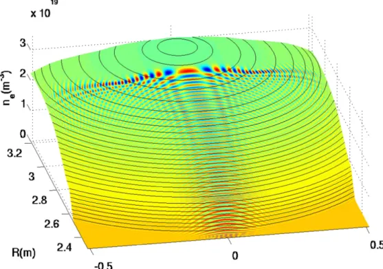
UFSR. In this section, instead of slab geometry we perform simulation with a realistic 2D geometry of the Tore-Supra tokamak(see figure9). We use a typical experimental density

profile, and the turbulence spectrum and amplitude used are based on the calculations done with a Helmholtz equation solver in a closed loop algorithm [20]. Figure10shows the turbulence spectrum that we used in these computations. To simulate realistic turbulence three isotropic homogeneous turbulence maps corresponding to different radial zones were mixed together using 2D shaped envelops for a smooth spectral transition. The 2D turbulence amplitude envelop depicted in figure 11, is based on experimental estimations has beenfitted with the following function.

d s s = + * -* * - + ( ) ( (( ) )) ( (( ) ) ) ( ) RMS n a b x x x x exp 2 0.5 tanh 0.5 12 m t 2 2

where a b, ,s s, 2 are fitting constants. The fitting function

(12) allows us to choose the edge turbulence amplitude by

changing parameter b. In the simulation presented here, the maximum edge RMS amplitude is equal to 1.9% from the highest probing frequency cut-off density which was chosen by us. The frequency sweep covers a radial zone of 12 cm in the plasma core. Another difference with the slab geometry computations is the turbulence correlation length. Here, the edge turbulence correlation length is 6 mm. Such a small correlation length can cause strong Bragg back-scattering. The poloidal plasma curvature makes the incident beam wider. The probing beam amplitude decays faster up to the cut-off vicinity region, which makes the diagnostic more sensitive to the edge turbulence with respect to core turbu-lence. In future large scale devices such as ITER, probing beam attenuation will be more pronounces what will increase even more sensitivity to the edge turbulence layer. Figure12

represents the signal phase variation spectrum for different edge turbulence amplitudes computed in a 2D toroidal cross-section, both with the IPF-FD3D full-wave code and

Figure 8.Complex signalfluctuation spectrum computed at different receiving antenna poloidal positions. The maximum RMS edge turbulence amplitude is 10% of the cut-off density.

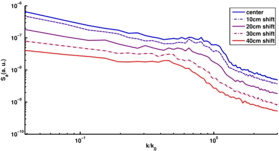
simplified weighting function approach. Here, we have the case of strong Bragg back-scattering. Scattering from the edge turbulence strongly changes phase variation spectral ampl-itude. The weighting function method fails to reliably describe the influence of the edge turbulence. Now let us see if it is possible to detect the presence of the edge turbulence amplitude peak in the reflectometer amplitude variation spectrum (see figure13). We can note that even with small

turbulence levels, it is possible to see a strong edge turbulence signature (the k-spectral peak observed in the spectrum) if on experimental setup we have small correlation lengths

and poloidal plasma curvatures. With a receiving antenna poloidal shift, the k-spectral peak shifts towards the direction of smaller wave-numbers, as observed in previous cases. With such a correlation length and turbulence level the beam widening due to the turbulence is not significant. However the beam widening produced by the poloidal plasma curvature can also have the same effect on the peak movement then a widening of the turbulence poloidal spectrum. In this case, it is not possible to measure turbulence properties by looking on the averaged receiving amplitude in antennas at different poloidal positions.

Figure 9.Contour maps of the probing wavefield superimposed with a 3D plot of the density profile.

6. Conclusions

Computations done both for slab geometry linear density profile and realistic Tore-Supra tokamak profile have shown the strong influence of the edge turbulence on core reflecto-metry measurements. This influence is expected to be even stronger in a large scale future devices as ITER. These effects are very complex and depend on the edge turbulence level, correlation length and plasma geometry. The simplified weighting function method is unable to describe phase var-iation spectrum change with edge turbulence level. The strong edge turbulence and the poloidal plasma curvature are pos-sible application limitations of the method. It is impospos-sible to measure strong edge turbulence directly with UFSR as in this case, probing beam behaviour is not proportional to the density variation and interpretation of such data is very complex. But it is still possible to detect strong edge turbu-lence by analyzing a reflectometer signal amplitude variation

from the plasma core. Enhanced beam scattering from the strong edge turbulence form spectral peaks in the signal amplitude variation spectrum. It is also possible to see the displacement of these spectral peaks when the receiving antenna is shifted in the poloidal direction away from the emitting antenna. The nature of these displacements is con-nected to the beam widening inside the strong edge turbu-lence layer. However, it must be pointed out that the reflectometer signal was calculated differently than in real experiments. Using the IPF-FD3D code, we simultaneously launch from the antenna all frequencies within the probing band and once the stationary solution is reached signal time series used to calculate amplitude and phase of the signal for each frequency. This way, the simulated signal is sensitive to back-scattering from areas located far away from the cut-off layer region. In real experiments the main reflection usually is filtered and the influence of back-scattering is smaller. So, the detection of strong edge turbulence peaks which were

Figure 11.Spatial evolution of the densityfluctuations profiles used as input for different cases of simulation.

Figure 12.Signal phase variation spectrum computed for different edge turbulence amplitudes.

observed in this work would require special analysis techni-ques for experimental signals. It was shown that coherent modes observed (characteristic peak appear in the phase variation spectrum) through strong edge turbulence. More-over, it was found that this peak is more pronounced in the amplitude variation spectrum then in phase variation spec-trum. The coherent mode spectral peak could be doubled resulting from thefirst scattering and second scattering after the cut-off reflection. With the receiving antenna poloidal misalignment a shift of thefirst scattering reflection peak in the direction of higher wave numbers was noticed.

ORCID iDs

G V Zadvitskiy https://orcid.org/0000-0002-3242-3089

C Lechte https://orcid.org/0000-0003-4171-888X

References

[1] Sabot R, Sirinelli A, Chareau J-M and Giaccalone J-C 2006 Plasma Physics Cont Fusion48 B421

[2] Morales R B, Hacquin S, Heuraux S and Sabot R 2017 Rev. Sci. Instrum88 043503

[3] Fanack C 1997 PhD Thesis Université Henri Poincaré, Nancy I [4] Heuraux S, Hacquin S, da Silva F, Clairet F, Sabot R and

Leclert G 2003 Rev. Sci. Instrum74 1501–6

[5] Gerbaud T, Clairet F, Sabot R and Sirinelli A 2006 Rev. Sci. Instrum.77 10E928

[6] Zadvitskiy G, Heuraux S, Lechte C, Hacquin S, Sabot R and Clairet F 2016 43rd EPS Conf. on Plasma Physics proceeding(http://ocs.ciemat.es/EPS2016PAP/pdf/P2.

013.pdf)

[7] Piliya A D and Popov A Y 2002 Plasma Phys. Control. Fusion

44 467

[8] Gusakov E Z and Popov A Y 2002 Plasma Phys. Control. Fusion44 2327

[9] Sysoeva E V, da Silva F, Gusakov E Z, Heuraux S and Popov A Y 2015 Nucl. Fusion55 033016

[10] Heuraux S and da Silva F 2012 Aims Journal Discrete and Continuous Dynamical Systems—Series S DCDS-S5

307–28

[11] Lechte C et al 2017 PPCF 59 PP075006

[12] Medvedeva A, Bottereau C, Clairet F, Hennequin P, Stroth U, Birkenmeier G, Cavedon M, Conway G D, Happel T and Heuraux S 2017 Plasma Phys. Control. Fusion59 125014 [13] da Silva F, Campos Pinto M, Despres B and Heuraux S 2015

J. Comp Phys295 24–45

[14] Bulanin V V, Petrov A V and Yefanov M V Consideration Doppler Reflectometry in Born Approximation IRW7 (Garching, Germany, 2010)(http://aug.ipp.mpg.de/IRW/ IRW7/papers/Bulanin-paper.pdf)

[15] Holzhauer E and Massig J H 1978 Plasma Phys.20 867

[16] Hornung G, Clairet F, Falchetto G L, Sabot R,

Arnichand H and Vermare L 2013 Plasma Phys. Control. Fusion55 12501311pp

[17] Prisiazhniuk D, Krämer-Flecken A, Conway G D, Happel T, Lebschy A, Manz P, Nikolaeva V, Stroth U and the ASDEX Upgrade Team 2017 Magneticfield pitch angle and perpendicular velocity measurements from multi-point time-delay estimation of poloidal correlation reflectometry Plasma Phys. Control. Fusion59 025013

[18] Krämer-Flecken A, Soldatov S, Xu Y, Arnichand H, Hacquin S, Sabot R and the TEXTOR team 2015 New J. Phys.17 073007

[19] Simon P, Conway G D, Stroth U, Biancalani A, Palermo F and the ASDEX Upgrade Team 2016 Plasma Phys. Control. Fusion58 045029

[20] Clairet F, Vermare L, Heuraux S and Leclert G 2004 12th International Congress on Plasma Physics 25-29(Nice, France) (https://arxiv.org/ftp/physics/papers/0410/ 0410212.pdf)

Figure 13.Signal amplitude variation spectrum computed at different receiving antenna poloidal positions in the case the highest edge turbulence level(RMS(dn nc)=1.8%).