HAL Id: hal-02465317
https://hal.archives-ouvertes.fr/hal-02465317
Submitted on 3 Feb 2020HAL is a multi-disciplinary open access archive for the deposit and dissemination of sci-entific research documents, whether they are pub-lished or not. The documents may come from teaching and research institutions in France or
L’archive ouverte pluridisciplinaire HAL, est destinée au dépôt et à la diffusion de documents scientifiques de niveau recherche, publiés ou non, émanant des établissements d’enseignement et de recherche français ou étrangers, des laboratoires
Space and time trade-off for the k shortest simple paths
problem
Ali Al Zoobi, David Coudert, Nicolas Nisse
To cite this version:
Ali Al Zoobi, David Coudert, Nicolas Nisse. Space and time trade-off for the k shortest simple paths problem. [Research Report] Inria & Université Cote d’Azur, CNRS, I3S, Sophia Antipolis, France. 2020. �hal-02465317�
Space and time trade-off for the k shortest simple paths problem
∗Ali Al-Zoobi1, David Coudert1, and Nicolas Nisse1 1Universit´e Cˆote d’Azur, Inria, CNRS, I3S, France
Abstract
The k shortest simple path problem (KSSP) asks to compute a set of top-k shortest simple paths from a vertex s to a vertex t in a digraph. Yen (1971) proposed the first algorithm with the best known theoretical complexity of O(kn(m + n log n)) for a digraph with n vertices and m arcs. Since then, the problem has been widely studied from an algorithm engineering perspective, and impressive improvements have been achieved.
In particular, Kurz and Mutzel (2016) proposed a sidetracks-based (SB) algorithm which is currently the fastest solution. In this work, we propose two improvements of this algo-rithm.
We first show how to speed up the SB algorithm using dynamic updates of shortest path trees. We did experiments on some road networks of the 9th DIMAC’S challenge with up to about half a million nodes and one million arcs. Our computational results show an average speed up by a factor of 1.5 to 2 with a similar working memory consumption as SB. We then propose a second algorithm enabling to significantly reduce the working memory at the cost of an increase of the running time (up to two times slower). Our experiments on the same data set show, on average, a reduction by a factor of 1.5 to 2 of the working memory.
1
Introduction
The classical k shortest paths problem (KSP) returns the top-k shortest paths between a pair of source and destination nodes in a graph. This problem has numerous applications in var-ious kinds of networks (road and transportation networks, communications networks, social networks, etc.) and is also used as a building block for solving optimization problems. Let D = (V, A) be a digraph, an s-t path is a sequence (s = v0, v1, · · · , vl = t) of vertices starting
with s and ending with t, such that (vi, vi+1) ∈ A for all 1 ≤ i < l. It is called simple if it has
no repeated vertices, i.e., vi 6= vj for all 0 ≤ i < j ≤ l. The length of a path is the sum of the
weights of its arcs and the top-k shortest paths is therefore the set containing a shortest s-t path, a second shortest s-t paths, etc. until the kth shortest s-t path.
Several algorithms for solving KSP have been proposed. In particular, Eppstein [5] proposed an exact algorithm that computes k shortest paths (not necessarily simple) with time complexity in O(m + n + k), where m is the number of arcs and n the number of vertices of the graph. An important variant of this problem is the k shortest simple paths problem (KSSP) introduced in 1963 by Clarke et al. [3] which adds the constraint that reported paths must be simple. This variant of the problem has various applications in transportation network when paths with
∗
This work has been supported by the French government, through the UCAjedi Investments in the Future
project managed by the National Research Agency (ANR) with the reference number ANR-15-IDEX-01, the ANR project MULTIMOD with the reference number ANR-17-CE22-0016, the ANR project Digraphs with reference number ANR-19-CE48-0013-01, and by R´egion Sud PACA.
repeated vertices are not desired by the user. It is also a subproblem of other important problems like constrained shortest path problem, vehicle and transportation routing [10, 12, 18]. It can be applied successfully in bio-informatics [1], especially in biological sequence alignment [16] and in natural language processing [2]. For more applications, see Eppstein’s recent comprehensive survey on k-best enumeration [6].
The algorithm with the best known time complexity for solving the (KSSP) problem has been proposed by Yen [19], with time complexity in O(kn(m + n log n)). Since, several works have been proposed to improve the efficiency of the algorithm in practice [7, 10, 11, 13, 15].
Recently, Kurz and Mutzel [14, 15] obtained a tremendous running time improvement, de-signing an algorithm with the same flavor as Eppstein’s algorithm. The key idea was to postpone as much as possible the computation of shortest path trees. To do so, they define a path using a sequence of shortest path trees and deviations. With this new algorithm, they were able to compute hundreds of paths in graphs with million nodes in about one second, while previous algorithms required an order of tens of seconds on the same instances. For instance, Kurz and Mutzel’s algorithm computed k = 300 hundred shortest paths in 1.15 seconds for the COL network [4] while it required about 80 seconds for the Yen’s algorithm and about 30 seconds by its improvement by Feng [7].
Our contribution. We propose two variations of the algorithm proposed by Kurz and Mutzel. We first show how to speed up their algorithm using dynamic updates of shortest path trees resulting with an average speed up by a factor of 1.5 to 2 and with a similar working memory consumption. We then propose a second algorithm enabling to significantly reduce the working memory at the cost of a small increase of the running time.
This paper is organized as follows. First, in Section 2.2, we describe Yen’s algorithm and then show in Section 2.3, how Kurz and Mutzel’s algorithm improves upon it. In Section 3, we present our algorithms by precisely describing how they differ from Kurz and Mutzel’s algorithm. Finally, Section 4 presents our simulation settings and results.
2
Preliminaries
2.1 Definition and Notation
Let D = (V, A) be a directed graph (digraph for short) with vertex set V and arc set A. Let n = |V | be the number of vertices and m = |A| be the number of arcs of D. Given a vertex v ∈ V , N+(v) = {w ∈ V | vw ∈ A} denotes the out-neighbors of v in D. Let wD : A → R+ be
a length function over the arcs. For every u, v ∈ V , a (directed) path from u to v in D is a sequence P = (v0 = u, v1, · · · , vr= v) of vertices with (vi, vi+1) ∈ A for all 0 ≤ i < r. Note that
vertices may be repeated, i.e., paths are not necessarily simple. A path is simple if, moreover, vi 6= vj for all 0 ≤ i < j ≤ r. The length of the path P equals wD(P ) = P06i<rwD(vi, vi+1)
(we will omit D when there is no ambiguity). The distance dD(u, v) between two vertices
u, v ∈ V is the shortest length of a u-v path in D (if any). Given two paths (v1, · · · , vr) and
Q = (w1, · · · , wp) and vrw1 ∈ A, let us denote the v1-wp path obtained by the concatenation of
the two paths by (v1, · · · , vr, Q).
Given s, t ∈ V , a top-k set of shortest s-t paths is any set S of (pairwise distinct) simple s-t paths such that |S| = k and w(P ) ≤ w(P0) for every s-t path P ∈ S and s-t path P0 ∈ S. The/ k shortest simple paths problem takes as input a weighted digraph D = (V, A), wD : A → R+
and a pair of vertices (s, t) ∈ V2 and asks to find a top-k set of shortest s-t paths (if they exist). Let t ∈ V . An in-branching T rooted at t is any sub-digraph of D that induces a tree containing t and such that every u ∈ V (T ) \ {t} has exactly one out-neighbor (that is, all paths go toward t). An in-branching T is called a shortest path (SP) in-branching rooted at t if, for
every u ∈ V (T ), the length of the (unique) u-t path PutT in T equals dD(u, t). Note that a SP
in-branching is sometimes called reversed shortest path tree.
In the forthcoming algorithms, the following procedure will often be used (and the key point when designing the algorithms is to limit the number of such calls and to optimize each of them). Given a sub-digraph H of D and u, t ∈ V (H), we use Dijkstra algorithm for computing a SP in-branching rooted in t that contains a shortest u-t path in H. Note that, the execution of the Dijkstra’s algorithm may be stopped as soon as a shortest u-t path has been computed (when u is reached), i.e., the in-branching may only be partial (i.e., not spanning D). The key point will be that this way to proceed not only returns a shortest u-t path in H (if any) but an SP in-branching rooted in t and containing u. Note that any such call has worst-case time complexity O(m + n log n).
Let P = (v0, v1, · · · , vr) be any path in D and i < r. Any arc a = viw 6= vivi+1 is called
a deviation of P at vi. Moreover, any path Q = (v0, · · · , vi, w, w1, · · · , w` = vR) is called an
extension of P at a (or at vi). Note that neither P nor Q is required to be simple. However, if
Q is simple, it will be called a simple extension of P at a (or at vi).
2.2 General framework: Yen’s algorithm and Feng’s improvements
We start by describing the general framework used by the KSSP algorithms in [7, 10, 11, 13, 15]. Precisely, let us describe Yen’s algorithm [19] trying to give its main properties and drawbacks. Then, we explain how Kurtz and Mutzel’s algorithm improves upon it (Section 2.3). Finally, we will detail our adaptation of the latter method in Section 3.
All of the algorithms described below start by computing a shortest s-t path P0 = (s =
v0, v1, · · · , vr = t) (in what follows we always assume that there is at least one such path).
This is done by applying Dijkstra’s algorithm from t (as described in previous section) and so also computes an SP in-branching T0 rooted at t and containing s. Note that P0 is simple since
weights are non-negative. Obviously, a second shortest s-t simple path must be a shortest simple extension of P0 at one of its vertices. Yen’s algorithm computes a shortest simple extension
of P0 at vi for every vertex vi in P0 as follows. For every 0 ≤ i < r, let Di(P0) be the graph
obtained from D by removing the vertices v0, · · · , vi−1 (this is to avoid non simple extension)
and the arc vivi+1 (to ensure that the computed path is a new one, i.e., different from P0). For
every 0 ≤ i < r, a SP in-branching rooted at t is computed using Dijkstra’s algorithm until it reaches vi and therefore returns a shortest path Qi from vi to t in Di(P0). Note that Yen’s
algorithm does not use further the SP in-branchings and this will be one key of the improvements described further. For every 0 ≤ i < r, the extension (v0, · · · , vi, Qi) of P0 at vi is added to a
set Candidate (initially empty). Note that the index i (called below deviation-index) where the path (v0, · · · , vi, Qi) deviates from P0 is kept explicit1. Once (v0, · · · , vi, Qi) has been added to
Candidate for all 0 ≤ i < r, by remark above, a shortest path in Candidate is a second shortest s-t simple path.
More generally, by induction on 0 < k0 < k, let us assume that a top-k0 set S of shortest s-t paths has been computed and the set Candidate contains a set of simple s-t paths such that there exists a shortest path Q ∈ Candidate such that S ∪ {Q} is a top-(k0+ 1) set of shortest s-t paths. Yen’s algorithm pursues as follows. Let Q = (v0 = s, · · · , vr = t) be any shortest path
in Candidate2 and let 0 ≤ j < r be its deviation-index. First, Q is extracted from Candidate and it is added to S (as the (k0+ 1)th shortest s-t path). Then, every shortest extension of Q is added to Candidate (since they are potentially a next shortest s-t path). For this purpose,
1The deviation-index is not kept explicitly in Yen’s algorithm but, since it is a trivial improvement already
existing in the literature, we mention it right now.
2Actually Candidate is implemented, using a pairing heap, in such a way that extracting a shortest path in
for every j ≤ i < r, let Di(Q) be the digraph obtained from D by first removing the vertices
v0, · · · , vi−1 (this is to avoid non simple extension). Then, here is one important bottleneck of
Yen’s algorithm, for every arc viw such that Candidate already contains some path with prefix
(v0, · · · , vi, w), then viw is removed from Di(Q). This therefore ensures to compute only new
paths. Indeed, the computed extensions are distinct from every path previously computed as they have different prefixes (this is the reason to keep explicitly the deviation-index). For every j ≤ i < r, a SP in-branching rooted at t is computed using Dijkstra’s algorithm until it reaches vi and therefore returns a shortest path Qi from vi to t in Di(Q). For every 0 ≤ i < r, the
extension (v0, · · · , vi, Qi) of Q at vi (together with its deviation index i) is added to the set
Candidate. This process is repeated until k paths have been found (when k0 = k).
Therefore, for each path Q that is extracted from Candidate, O(|V (Q)|) applications of Dijkstra’s algorithm are done. This gives an overall time-complexity of O(kn(m + n log n)) which is the best theoretical (worst-case) time-complexity currently known (and of all algorithms described in this paper) to solve the k-shortest paths problem.
One expensive part in the pre-described framework of Yen’s algorithm is the multiple calls of Dijkstra’s algorithm. Feng [7] proposed a practical improvement by trying to avoid some calls. Essentially, when a path Q = (v0, · · · , vr) with deviation-index j is extracted, its extensions are
computed from i = j to r − 1. Roughly, for every j < i ≤ r, the computation of the extension at vi is actually done with the help of the initial SP in-branching T0. In practice, this process
accelerates significantly the executions of Dijkstra’s algorithm. At the price of a larger memory consumption, Kurz and Mutzel improved Yen’s framework which leads to the current fastest algorithm (Section 2.3) for the k shortest simple paths problem.
2.3 Kurz and Mutzel’s algorithm
All of Yen’s improvements aim at minimizing the time consumed by Dijktra’s algorithm calls. Instead, Kurz and Mutzel [15] chose to use a smaller number of such calls. This can be done by memorizing the SP in-branchings previously computed by the algorithm. More precisely, instead of keeping the paths in the set Candidate, the algorithm keeps only a representation of it using a sequence of SP in-branchings and deviations. These representations will allow to extract any shortest path P in time O(|P |) and the length of P in constant time. As a result, for each shortest s-t path P , the memorized SP in-branching can be used to extract a shortest extension of P at a vertex vi in a pivot step. Unfortunately, there is no guarantee that the
extracted shortest extension will be simple. If it is not simple, a new Dijsktra’s algorithm call has to be done. However, in many cases the extracted extension is simple and a Dijsktra’s algorithm call can be avoided.
Precisely, Kurz and Mutzel’s algorithm mainly relies on two keys improvements. First, following a principle of Eppstein’s algorithm [5], it explicitly keeps the SP in-branchings com-puted during the execution of the algorithm (this is at some non-negligible cost of working memory consumption, but leads to an improvement of the practical running-time). Moreover, instead of computing the extensions of the extracted path at each iteration, the algorithm adds to Candidate a representation of each extension (together with a lower bound of its length). Then, only when such a representation is extracted from Candidate, the corresponding ex-tension is explicitly computed. This way of postponing the computations allows to avoid the actual computation of many extensions (whose never be used further), which leads to a drastic improvement of the running time.
Let us describe the Kurz and Mutzel’s algorithm whose pseudo code is given in Algorithm 1. As usual, the algorithm starts with the computation of a shortest s-t (simple) path P0 =
Algorithm 1 Kurz-Mutzel Sidetrack Based (SB) algorithm for the KSSP [15] Require: A digraph D = (V, A), a source s ∈ V , a sink t ∈ V , and an integer k Ensure: k shortest simple s-t paths
1: Let Candidatesimple← ∅, Candidatenot−simple← ∅, ← ∅ and Output ← ∅
2: T0 ← a SP in-branching of D rooted at t containing s
3: Add ((T0), w(Pst(T0))) to Candidatesimple
4: while Candidatesimple∪ Candidatenot−simple 6= ∅ and |Output| < k do
5: ε = ((T0, e0, · · · , Th, eh = (uh, vh), Th+1), lb) ← a shortest element in Candidatesimple
and Candidatenot−simple // with priority to Candidatesimple
6: if ε ∈ Candidatesimple then
7: Extract ε from Candidatesimple and add it to the Output
8: for every deviation e = (vj, v0) with vj ∈ Pvht(Th+1) do
9: ext ← (T0, e0, · · · , Th, eh, Th+1, e, Th+1)
10: lb0← lb − w(Pvjt(Th+1)) + w(e) + w(Pv0t(Th+1))
11: if ext represents a simple path then 12: Add (ext, lb0) to Candidatesimple
13: else
14: T0 ← the name of a SP in-branching of Dh(P ) // T0 is not computed yet
15: Add T0 to
16: Add ((T0, e0, · · · , Th, eh, Th+1, e, T0), lb0) to Candidatenot−simple
17: else
18: if Th+1has not been computed yet then
19: Compute Th+1, a SP in-branching of Dh(P ) and add it to
20: ε0= ((T0, e0, · · · , Th, eh, Th+1), lb + w(Pv0t(Th+1)) − w(Pv0t(Th)))
21: Add ε0 to Candidatesimple
22: return Output
s. T0 is added to a set initially empty (this set will contain all computed SP in-branchings).
Then, for every 0 ≤ i < r, and for every deviation e at vi (i.e., arcs e = viw are considered
for every w ∈ N+(vi) \ {v0, · · · , vi+1}), let Pwt(T0) be the shortest path from w to t in T0.
Note that the path Q(i, e) = (v0, · · · , vi, w, Pwt(T0)) is a shortest extension of P0 at e, but it
is not necessarily simple (it is not simple if Pwt(T0) intersects {v0, · · · , vi}). Hence, lb(e) =
w((v0, · · · , vi)) + w(viw) + w(Pwt(T0)) is a lower bound on the length of any shortest simple
extension of P0 at e (and it is its actual length if the path Q(i, e) is simple). The algorithm
proceeds as follows. First, by categorizing the vertices of T0 (using a trick due to Feng [7] that
we do not detail here), it is possible to decide in constant time, for each i < r and each deviation e at vi, whether Q(e, i) is simple or not. Then, for every 0 ≤ i < r, and for every deviation e at
vi, the algorithm adds ((T0, e, T0), lb(e)) in a heap (ordered using lb) Candidatesimple if Q(e, i)
is simple, and it adds ((T0, e, Ti), lb(e)) in a heap Candidatenot−simple otherwise, where Ti is
the name of a new SP in-branching rooted at t in D \ {v0, · · · , vi} whose actual computation
is postponed. Hence, T0 is the only SP in-branching that has been computed (using Dijkstra’s
algorithm) so far.
More generally, by induction on 0 < k0 < k, let us assume that a top-k0 set S of shortest s-t paths and two heaps Candidatesimple and Candidatenot−simple have been computed. Following
Eppstein’s idea, each element of these heaps is of the form ((T0, e0, · · · , Th, eh, Th+1), lb)
(describ-ing a path explained below) such that, for every 0 ≤ i ≤ h, Ti is a SP in-branching that has
Th+1 may not have already been computed but has a pointer associated to it stored in . That
is, even if Th+1 has not yet been computed, it is defined and can be referred to. Observe that
we may have Tj = Tj+1 for some 0 ≤ j ≤ h + 1.
Let P1 be the simple path that starts in s and, for every 0 ≤ j ≤ h, follows the (already
computed) tree Tj from the current vertex till the tail of deviation ej and then follows deviation
ej to its head. Hence, P1 ends in the head z of eh. Now, if the element is in Candidatesimple,
we know by induction that the SP in-branching Th+1 has already been computed and that
the path P obtained by concatenating P1 and the shortest z-t path Pzt(Th+1) is guaranteed
to be simple and has length w(P ) = w(P1) + w(Pzt(Th+1)) = lb(eh). If the element is in
Candidatenot−simple (the shortest z-t path Pzt(Th) intersects P1) the algorithm actually
com-putes the SP in-branching Th+1rooted at t (if not already done). Observe that the digraph in
which Th+1is computed is a subdigraph of the digraph in which Th has been computed, and so
w(Pzt(Th+1)) ≥ w(Pzt(Th)) (by setting w(Pzt(Th+1)) = +∞ if there is no z-t path in Th+1) and
z is the only common vertex of P1 and Pzt(Th+1). Hence, the path P obtained by concatenating
P1 and the shortest z-t path Pzt(Th+1) (if it exists) is guaranteed to be simple and has length
w(P ) = w(P1) + w(Pzt(Th+1)) ≥ w(P1) + w(Pzt(Th)) = lb(eh).
An iteration of Kurz and Mutzel’s algorithm proceeds as follows. First an element ε = ((T0, e0, T1, e1, · · · , Th, eh, Th+1), lb) with smallest lb is extracted from Candidatesimple and
Candidatenot−simple (with priority for Candidatesimple in case of equal lb). If ε was in
Candidatesimple, the path P as defined above is the next shortest simple s-t path and it is added
to the output. Then, all possible deviations of P along the path Pzt(Th+1) are determined and
added to Candidatesimple or Candidatenot−simple depending on whether they are simple or not
(note that only a representation of them is build and not the actual path). Otherwise, the algorithm actually computes the SP in-branching Th+1 (if not already done) to determine the
shortest z-t path in Th+1 (if it exists), and adds Th+1 to . If such path exists, the algorithm
adds to Candidatesimplea new element ((T0, e0, T1, e1, · · · , Th, eh, Th+1), lb0) describing a simple
s-t path with length lb0 = w(P1) + w(Pzt(Th+1)) = lb − w(Pzt(Th)) + w(Pzt(Th+1)).
Actually, the same SP in-branching can be used for all deviations at the same vertex vi of
a given path P . So, for each vertex vi in P , a single call of Dijkstra’s algorithm is needed.
As a result, finding all of the extensions of a given path P can be done in O(|P |(m + n log n)) time. Therefore, the time complexity of Kurz and Mutzel’s algorithm (in the worst case) is bounded by O(kn(m + n log n)) as the algorithm extends no more than k paths and the number of vertices of each path is bounded by n.
Overall, Kurz and Mutzel’s algorithm computes k shortest simple s-t paths with a much fewer number of applications of Dijkstra’s algorithm and so its running time is in general much better than the algorithms proposed by Yen or Feng. On the other hand, it requires to store many SP in-branchings previously computed which implies a larger working memory consumption.
3
Our contributions
We propose two independent variants of SB algorithm (Algorithm 1). The first algorithm, called SB*, gives, with respect to our experimental results, an average speed up by a factor of 1.5 to 2 compared with SB algorithm. Our second algorithm, called PSB (Parsimonious SB), is based on a different manner to handle non simple candidates in order to reduce the number of computed and stored SP in-branchings. This leads to a significant reduction of the working memory at the price of a slight increase of the running time compared with SB algorithm.
3.1 The SB* algorithm
Here, we propose a variant of the SB algorithm, strongly based on Kurz and Mutzel’s framework, that is a tiny modification of SB algorithm allowing to speed it up.
More precisely, each time a representation (T0, e0, T1· · · , eh−1 = (uh−1, vh−1), Th, eh =
(uh, vh), Th+1) is extracted from Candidatenot−simple and that Th+1 has not been computed
yet (i.e., it is only a pointer), our algorithm does not compute Th+1 from scratch as SB
algo-rithm does. Instead, SB* algoalgo-rithm creates a copy T of Th, discards vertices of the path from
vh−1 to uh in Th, and updates the SP in-branching T using standard methods for updating a
shortest path tree [9]. Then, the pointer Th+1is associated to the new in-branching T .
It is clear that the SB* algorithm computes (and store) exactly the same number of in-branchings as SB algorithm. The computational results presented in Section 4.2 show that this update procedure gives an average speed up by a factor of 1.5 to 2.
3.2 The PSB algorithm
Our main contribution is the Parsimonious SB algorithm (PSB) presented in this section whose main goal is to solve the k shortest simple paths problem with a good tradeoff between the running time and the working memory consumption. Indeed, a weak point of the SB algorithm comes from the fact that it keeps in the memory all the SP in-branchings that it computes throughout its execution. In order to reduce the working memory consumption, the main difference between the SB algorithm and the one presented here consists of the types of the elements that PSB algorithm stores in the heap Candidatenot−simple and the way they are used.
We now describe PSB algorithm by detailing how its differs from SB algorithm. Let us mention that PSB algorithm uses a heap Candidatesimple similar (i.e., containing exactly the same type
of elements) to the one used by SB algorithm.
Let us start considering a step of PSB algorithm when an element ε = ((T0, e0, T1, e1, · · · ,
Th, eh= (uh, vh), Th+1), lb) is extracted from Candidatesimple. The first difference between the
SB algorithm is that Th+1may have not yet been computed, in which case it must be computed
at that step and stored in . Next, as the SB algorithm, the PSB algorithm first adds the (simple) path P corresponding to ε to the output. Then, it considers all deviations of P at the vertices between vh and t, i.e., all arcs (not in P ) with tail in Pvht(Th+1). For every such
deviation e = (u, v) with u ∈ V (Pvht(Th+1)), by using the Feng’s “trick” (already mentioned
without details), it can be decided in constant time whether it admits a simple extension, i.e., whether the path Pe that “follows” the path P1 corresponding to ε from s to vh, then follows
the path Pvhu(Th+1), the arc e and finally the path Pvt(Th+1) is simple or not. In the case
when Pe is simple, then the element ((T0, e0, T1, e1, · · · , Th, eh, Th+1, e, Th+1), lbe) is added to
Candidatesimple, where lbe = w(P1) + w(Pvhu(Th+1)) + w(e) + w(Pvt(Th+1)) (exactly as it is
done by the SB algorithm). The second difference with the SB algorithm relies on the set X = {f1, · · · , fr} of deviations for which the extension using Th+1 is not simple. The key
point is that we create a single element for all deviations in X. This ensures that the size of Candidatenot−simple is at most k, as at most one element is added to Candidatenot−simple per
path added to the output. More precisely, let X = {f1, · · · , fr} be the set of “non simple”
deviations ordered in such a way that, for every 1 ≤ i < j < l ≤ r, the tail of fj is between (or
equal to) the tails of fi and fl on the path Pvht(Th+1). For every 1 ≤ i ≤ r and fi = uivi, let
lbi = lbfi = w(P1) + w(Pvh,ui(Th+1)) + w(fi) + w(Pvi,t(Th+1)). The PSB algorithm then adds
the element ε0= ((T0, e0, T1, e1, · · · , Th, eh, Th+1, X, Th+1), min1≤i≤rlbi) to Candidatenot−simple,
and so the weight of ε0 in the heap Candidatenot−simple is the smallest lower bound among all
lower bounds related to the “non simple” deviations in X.
Candidatenot−simple. This happens, as in the SB algorithm, when the smallest key (lower
bound) of the elements in Candidatesimple∪ Candidatenot−simple corresponds only to an
el-ement of Candidatenot−simple. Let ε = ((T0, e0, T1, e1, · · · , Th, eh, Th+1, X, Th+1), lb) be this
element and let X = {f1, · · · , fr}. Let also eh = uhwh, let P1 = (s = x1, · · · , xo = wh) be the
prefix (from s to wh) of the path represented by ε, let Pwht(Th+1) = (wh, wh+1, · · · , wp= t) and
let fj = wijvj for every 1 ≤ j ≤ r (by the way the fj’s are ordered, h ≤ ij ≤ ij0 ≤ p for all
1 ≤ j ≤ j0 ≤ r). The fact that the type of the elements in Candidatenot−simple is more involved (so, allowing to decrease a lot the working memory) requires more involved (and potentially more costly in term of running time) way to treat them. To limit the increase of the running time, the PSB algorithm proceeds in such a way that several deviations in {f1, · · · , fr} are
somehow considered “simultaneously”. More precisely, it proceeds as follows.
Let 1 ≤ i∗ ≤ r be the smallest integer i such that lbi = lb. The PSB algorithm
pro-ceeds as follows to deal with the deviations fr, fr−1, · · · , fi∗ in this order. First, it applies
Dijkstra’s algorithm to compute a SP in-branching Tr0 rooted at t in Dr = D − {x1, · · · , xo =
wh, · · · , wir} until it reaches vr. If vr is reached, then the path Qr = P1Pwhwir(Th+1)Pvrt(T
0 r)
is a simple s-t path and the element ((T0, e0, T1, e1, · · · , Th, eh, Th+1, fr, Tr0), w(Qr)) is added
to Candidatesimple. However, the in-branching Tr0 is not saved into but only its name is kept
(this allows to reduce the working memory size while it may require to recompute the tree Tr0 later. The bet here is that it will not be necessary to actually redo this computation). Then, for j = r − 1 down to i∗, the SP in-branching Tr0 is updated to become the SP in-branching Tj0 rooted in t in Dj = D − {x1, · · · , xo = wh, · · · , wij}, possibly reaching vj and so
providing a simple path Qj. To speed up the computation of Tj0, it is actually computed by
updating Tj+10 which is done using standard methods for updating a shortest path tree [9]. Fi-nally, the element ((T0, e0, T1, e1, · · · , Th, eh, Th+1, fj, Tj0), w(Qj)) is added to Candidatesimple.
In the current implementation of our PSB algorithm (the one used in the experiments de-scribed in next section), the in-branching Tj0 is saved in only if j = i∗3. Finally, the element ((T0, e0, T1, e1, · · · , Th, eh, Th+1, X0, Th+1), min1≤j<i∗lbj), with X0 = {f1, · · · , fi∗−1}, is added
into Candidatenot−simple.
The correctness of the PSB algorithm follows from the one of the SB algorithm by notic-ing that the elements extracted from Candidatesimple∪ Candidatenot−simple are the ones with
smallest lower bound and the fact that, each time that a path is extracted, a shortest extension of each of its deviations is considered.
Finally, as already mentioned, the number of elements in the heap Candidatenot−simple is
bounded by k as each of its elements correspond to a path that has been added to the output, while with the SB algorithm, this heap may contain O(km) elements. Furthermore, as for the SB algorithm, we may keep only the k elements with smallest lower bound in Candidatesimple.
Hence, the working memory used by the PSB algorithm for the heaps is significantly smaller than for the SB algorithm. However, the largest part of the working memory is due to the number of SP in-branchings that are computed and stored in . Although this number seems difficult to evaluate, we observe experimentally (see Section 4) that it is significantly smaller with the PSB algorithm.
3
A better way to establish an even better tradeoff between space and time would be to determine a good threshold τ such that an in-branching Tj0 is stored in if and only if w(Qj) ≥ τ . Due to lack of time we have not
Area ROME DC DE NY BAY COL Number of vertices 3 353 9 559 49 109 264 346 321 270 435 666 Number of edges 8 870 29 682 119 520 733 846 800 172 1 057 066
Table 1: Characteristics of the TIGER graphs used in KSSP experiments.
4
Experimental evaluation
4.1 Experimental settings
We have implemented4the algorithms NC (improvement of Yen’s algorithm by Feng [7]), SB [15], SB* and PSB in C++14 and our code is publicly available at https://gitlab.inria.fr/ dcoudert/k-shortest-simple-paths.
Following [15], we have implemented a pairing heap data structure [8] supporting decrease key operation, and we use it for the Dijkstra shortest path algorithm. Our implementation of the Dijkstra shortest path algorithm is lazy, that is it stops computation as soon as the distance from query node v to t is proved to be the shortest one. Further computations might be performed later for another node w at larger distance from t. Our implementation of Dijkstra’s algorithm supports update operation when a node or an arc is added to the graph. In addition, we have implemented a special copy operation that enables to update the in-branching when a set of nodes are removed from the graph. This corresponds to the operations performed when creating an in-branching Th+1 from Th. Observe that in our implementations of NC, SB, SB*
and PSB, the parameter k is not part of the input, and so the sets of candidates are simply implemented using pairing heaps. This choice enables to use these methods as iterators able to return the next shortest path as long as one exists. We have evaluated the performances of our algorithms on some road networks from the 9th DIMACS implementation challenge [4]. The characteristics of these graphs are reported in Table 1. In the following, we refer to the graphs ROME, DC and DE as the small networks, and to the graphs NY, BAY and COL as the large networks. We also generated random networks using method RandomGNM of SageMath [17] with n ∈ {5000, 10000, 20000} and for each n, we let m = 10n, 50n and 100n. For each network (both the random and the road networks), we have measured the execution time and the number of SP in-branching computed (as it can be used to measure the memory consumption). For each network we run the algorithms on a thousand pairs of vertices randomly chosen. In the tables below we report the average and the median of their time consumption / number of stores SP in-branching.
All reported computations have been performed on computers equipped with 2 quad-core 3.20GHz Intel Xeon W5580 processors and 64GB of RAM.
4.2 Experimental results
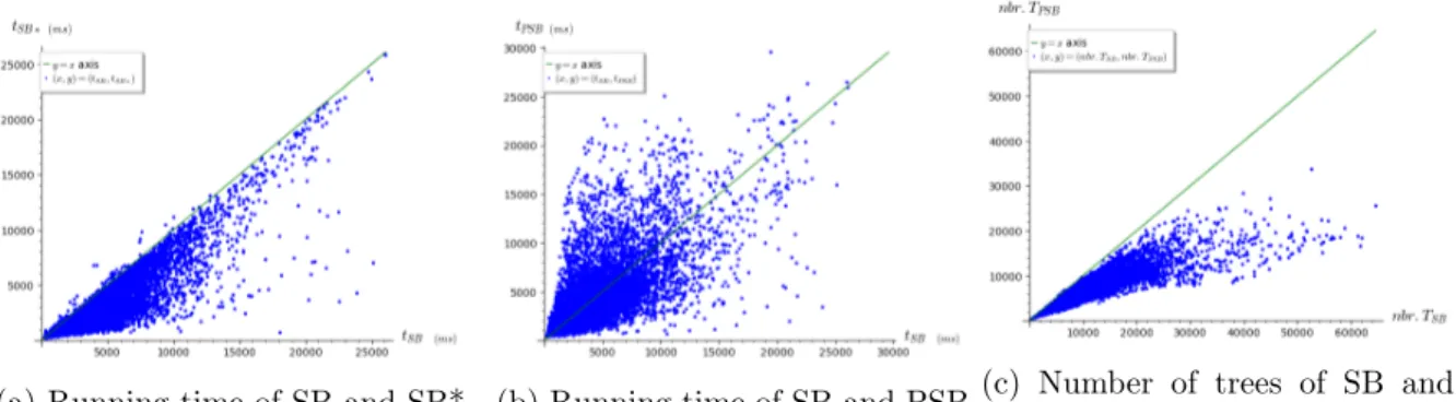
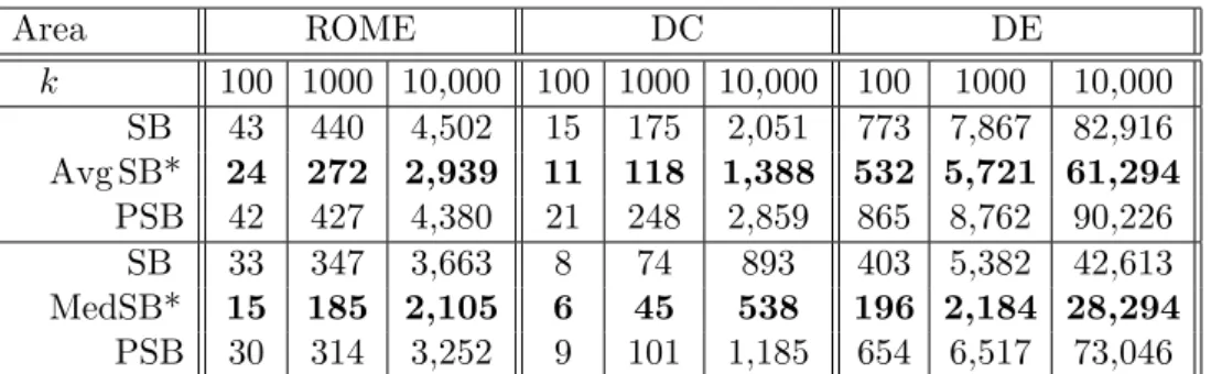
The simulations show that our tiny improvement SB* of SB algorithm allows to decrease the running-time by a factor between 1,5 (on ROME) and 2 (on COL) in average (Tables 2 and 3). In particular, in all the networks considered, SB* algorithm is, for most of the queries, faster than SB algorithm (Figures 1a and 2a). By design, the number of in-branchings that are stored is the same in both algorithms. It is interesting to note that the gain increase with the size of the networks. It seems that the differences of performances depends on the structure of the queries and of the networks. It will be an interesting further work to better understand the relationship between the kinds of queries and/or networks and the gain in running time.
4
The simulations comparing PSB algorithm and SB algorithm show a significant reduction of the working memory when using PSB (Tables 4 and 5 and Figures 1c and 2c). Again, the gain increases when considering larger networks. In term of running time, SB algorithm is slightly faster in average but Figures 1b and 2b indicate that globally, they are quite comparable. It would be interesting to understand the impact of the length of the queries on the performances of both algorithms.
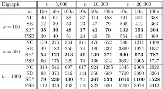
Finally, following some simulations in [15], we have also compared all the algorithms on random graphs (Ed¨os-R´enyi). Due to lack of time, we considered only one graph per setting (number of vertices, of edges and k) and the average is done on 1000 requests (note that this setting is similar to the one in [15]). The performances (Table 6) are similar than in the ones obtained for road networks. That is, SB* algorithm is faster than all other algorithms (more than twice faster in the case of large graphs when k = 1000). Surprisingly, the NC algorithm is sometimes (for dense graphs) faster than SB and PSB. Moreover, PSB algorithm always uses less memory than SB algorithm (Table 7), with a more significant difference in the case of sparse large graphs.
In the future work, we will continue our experiments in order to discover which conditions (structure of graphs and queries...) make one of the prescribed algorithms faster or / and less memory consuming than the others.
(a) Running time of SB and SB* (b) Running time of SB and PSB(c) Number of trees of SB and PSB
Figure 1: Comparison of the running time of SB versus SB* (fig. 1a) and SB versus PSB (fig. 1b) on ROME, and comparison of the number of stored tree for SB versus PSB (fig. 1c). Each dot corresponds to one pair source/destination.
(a) Running time of SB and SB* (b) Running time of SB and PSB(c) Number of trees of SB and PSB
Figure 2: Comparison of the running time of SB versus SB* (fig. 2a) and SB versus PSB (fig. 2b) on COL, and comparison of the number of stored tree for SB versus PSB (fig. 2c). Each dot corresponds to one pair source/destination.
Area ROME DC DE k 100 1000 10,000 100 1000 10,000 100 1000 10,000 Avg SB 43 440 4,502 15 175 2,051 773 7,867 82,916 SB* 24 272 2,939 11 118 1,388 532 5,721 61,294 PSB 42 427 4,380 21 248 2,859 865 8,762 90,226 Med SB 33 347 3,663 8 74 893 403 5,382 42,613 SB* 15 185 2,105 6 45 538 196 2,184 28,294 PSB 30 314 3,252 9 101 1,185 654 6,517 73,046
Table 2: Time consuming (average and median in ms) of SB, SB* and PSB on small networks
Area NY BAY COL
k 100 500 1000 100 500 1000 100 500 1000 Avg SB 904 4,334 8,741 3,270 18,464 38,346 5,216 28,262 59,717 SB* 581 2,787 5,707 2,395 13,669 28,545 3,723 20,313 43,373 PSB 1,822 9,417 19,166 5,083 27,438 55,711 7,371 39,078 80,696 Med SB 156 600 1,230 695 4,073 9,443 1,412 8,737 19,664 SB* 148 356 676 340 2,075 4,934 722 5,051 11,620 PSB 336 2,324 5,278 1,934 12,000 25,760 3,072 19,219 42,114
Table 3: Time consuming (average and median in ms) of SB,SB* and PSB on big networks
Area ROME DC DE k 100 1000 10,000 100 1000 10,000 100 1000 10,000 Avg SB 106 1,108 11,446 14.9 209 2,594 88 928 9,945 PSB 53 667 6,956 10.6 140 1,716 36 390 4,212 MedSB 87 961 10,164 6 105 1,555 48 557 6,551 PSB 56 615 6,570 5 80 1,106 25 287 3,154
Table 4: Number of SP in-branching genereted and stored by SB and PSB on small networks
Area NY BAY COL
k 100 500 1000 100 500 1000 100 500 1000
Avg SB 14.9 81 171 44.6 266 562 47 266 570
PSB 9.8 51 106 22 124 259 22 123 259
MedSB 3 21 45 13 90 209 13 101 234
PSB 2 16 35 9 57 124 9 63 142
Digraph n = 5, 000 n = 10, 000 n = 20, 000 m 10n 50n 100n 10n 50n 100n 10n 50n 100n k = 100 NC 40 64 88 37 114 158 191 304 388 SB 12 39 53 23 47 79 805 412 363 SB* 35 30 48 17 41 70 132 153 204 PSB 30 40 51 24 46 78 554 435 389 k = 500 NC 159 275 354 311 470 652 789 1211 1498 SB 49 182 250 74 180 332 3869 1924 1637 SB* 54 121 213 40 139 271 690 573 787 PSB 66 175 229 74 166 314 3692 2005 1727 k = 1000 NC 313 546 697 617 924 1285 1545 2368 2920 SB 98 370 512 144 356 669 7709 3890 3264 SB* 79 239 430 71 267 533 1010 1100 1528 PSB 112 349 463 145 322 620 5209 3978 3412
Table 6: Average time consuming (in ms) of NC,SB, SB* and PSB on random digraph with different densities Digraph n = 5, 000 n = 10, 000 n = 20, 000 m 10n 50n 100n 10n 50n 100n 10n 50n 100n k = 100 SB 2.332 3.726 2.08 1.992 1.566 1.753 33.142 9.149 5.09 PSB 2.275 3.657 2.04 1.952 1.538 1.724 25.95 8.529 4.882 k = 500 SB 8.88 16.07 7.477 6.287 4.615 5.493 161.844 42.866 22.094 PSB 8.434 15.57 7.175 6.041 4.465 5.269 126.23 39.603 21.018 k = 1000 SB 17.477 32.207 14.98 12.023 8.623 10.532 323.231 85.178 43.193 PSB 16.538 31.132 14.34 11.471 8.307 10.059 252.151 78.28 40.948
Table 7: Average of number of SP in-branching computed and stored using SB and SB* on random digraph with different densities
References
[1] Arita, M. Metabolic reconstruction using shortest paths. Simulation Practice and Theory 8, 1-2 (2000), 109–125.
[2] Betz, M., and Hild, H. Language models for a spelled letter recognizer. In 1995 International Conference on Acoustics, Speech, and Signal Processing (1995), vol. 1, IEEE, pp. 856–859.
[3] Clarke, S., Krikorian, A., and Rausen, J. Computing the n best loopless paths in a network. Journal of the Society for Industrial and Applied Mathematics 11, 4 (1963), 1096–1102.
[4] Demetrescu, C., Goldberg, A., and Johnson, D. 9th dimacs implementation chal-lenge - shortest paths, 2006.
[5] Eppstein, D. Finding the k shortest paths. SIAM Journal on Computing 28, 2 (1998), 652–673.
[6] Eppstein, D. k-best enumeration. arXiv preprint arXiv:1412.5075 (2014).
[7] Feng, G. Finding k shortest simple paths in directed graphs: A node classification algo-rithm. Networks 64, 1 (2014), 6–17.
[8] Fredman, M. L., Sedgewick, R., Sleator, D. D., and Tarjan, R. E. The pairing heap: A new form of self-adjusting heap. Algorithmica 1, 1 (1986), 111–129.
[9] Frigioni, D., Marchetti-Spaccamela, A., and Nanni, U. Fully dynamic algorithms for maintaining shortest paths trees. J. of Algorithms 34, 2 (2000), 251 – 281.
[10] Hadjiconstantinou, E., and Christofides, N. An efficient implementation of an algorithm for finding k shortest simple paths. Networks: An International Journal 34, 2 (1999), 88–101.
[11] Hershberger, J., Maxel, M., and Suri, S. Finding the k shortest simple paths: A new algorithm and its implementation. ACM Transactions on Algorithms (TALG) 3, 4 (2007), 45.
[12] Jin, W., Chen, S., and Jiang, H. Finding the k shortest paths in a time-schedule network with constraints on arcs. Computers & operations research 40, 12 (2013), 2975– 2982.
[13] Katoh, N., Ibaraki, T., and Mine, H. An efficient algorithm for k shortest simple paths. Networks 12, 4 (1982), 411–427.
[14] Kurz, D. k-best enumeration - theory and application. Theses, Technischen Universit¨at Dortmund, Mar. 2018.
[15] Kurz, D., and Mutzel, P. A sidetrack-based algorithm for finding the k shortest simple paths in a directed graph. In Int. Symp. on Algorithms and Computation (ISAAC) (2016), vol. 64 of LIPIcs, Schloss Dagstuhl, pp. 49:1–49:13.
[16] Shibuya, T., and Imai, H. New flexible approaches for multiple sequence alignment. Journal of Computational Biology 4, 3 (1997), 385–413.
[17] The Sage Developers. SageMath, the Sage Mathematics Software System (Version 8.9), 2019. https://www.sagemath.org.
[18] Xu, W., He, S., Song, R., and Chaudhry, S. S. Finding the k shortest paths in a schedule-based transit network. Computers & Operations Research 39, 8 (2012), 1812–1826.
[19] Yen, J. Y. Finding the k shortest loopless paths in a network. Management Science 17, 11 (1971), 712–716.