HAL Id: cea-02339870
https://hal-cea.archives-ouvertes.fr/cea-02339870
Submitted on 5 Nov 2019HAL is a multi-disciplinary open access
archive for the deposit and dissemination of sci-entific research documents, whether they are pub-lished or not. The documents may come from teaching and research institutions in France or abroad, or from public or private research centers.
L’archive ouverte pluridisciplinaire HAL, est destinée au dépôt et à la diffusion de documents scientifiques de niveau recherche, publiés ou non, émanant des établissements d’enseignement et de recherche français ou étrangers, des laboratoires publics ou privés.
Water experiment for assessing vibroacoustic
beamforming gain for acoustic leak detection in a
sodium-heated steam generator
S. Kassab, L. Maxit, F. Michel
To cite this version:
S. Kassab, L. Maxit, F. Michel. Water experiment for assessing vibroacoustic beamforming gain for acoustic leak detection in a sodium-heated steam generator. Mechanical Systems and Signal Processing, Elsevier, 2018, 134, pp.106332. �10.1016/j.ymssp.2019.106332�. �cea-02339870�
Water experiment for assessing the vibroacoustic beamforming gain in the
framework of the acoustic leak detection for the sodium-heated steam generator
Souha Kassab 1,2, Frédéric Michel2, Laurent Maxit1
1. INSA–Lyon, Laboratoire Vibrations-Acoustique (LVA), 25 bis, av. Jean Capelle, F-69621, Villeurbanne Cedex, France.
e-mail: laurent.maxit@insa-lyon.fr (corresponding author)
2. CEA, DEN,DTN/STPA/LISM, F-13115 Saint-Paul-lez-Durance, France.
Abstract: In an intent to improve the monitoring of steam generators, a technique based on vibration measurements is developed for the detection of a water leak into sodium. Background noise can mask the leak-induced vibrations. In order to increase the signal-to-noise ratio (SNR), a beamforming technique may be considered. In the purpose of studying the feasibility and the efficiency of this technique for the present configuration, experimental investigations have been performed on a mock-up composed by a straight cylindrical pipe coupled to a hydraulic circuit through two flanges. A sound emitter introduced in the pipe simulates the source to detect, whereas a flow speed controls the background noise vibrations. Beamforming is applied on the signals measured by an array of accelerometers externally mounted on the pipe. Two different kinds of beamforming are considered: the conventional (Bartlett) one and an advanced one based on SNR maximization (MaxSNR). After an analysis of the vibroacoustic behaviour of the mock-up, one studies the efficiency of the two beamforming treatments for narrow bands and broad bands.
Keywords: sodium-heated steam generator, leak detection, beamforming, array gain, structural acoustics, heavy fluid.
1. Introduction
This paper describes the study of a non-intrusive vibroacoustic beamforming technique aimed at the detection of sodium-water reactions in the steam generator unit (SGU) of a liquid sodium fast reactor (SFR). Early detection is important since sodium/water reaction may conduct to severe damage if appropriate action is not taken quickly. In the past, different works considering active (Cavaro et al. 2010) and passive (Chikazawa 2010) detection techniques have been carried out. The passive techniques are based on the fact that the high difference of pressure
and the strong sodium/water chemical reaction caused by the leak make acoustic noise. As the propagation time of the acoustic wave from the leak to sensors on the external surface of the SGU is sufficiently small, acoustic techniques can be used to detect the leak in a short time. These methods are however strongly sensitive to the background noise caused by the sodium and water flows, the water boiling and the vibrations induced by the pumps. Kim et al. (2010) studied the noise spectrum induced by the sodium-water reaction for various leak rates lower than 1 g/s. They concluded a small leak at a rate of 0.4 to 0.6 g/s generates a wide band of 1 to 200 kHz noise, which can be detected using a single sensor and a threshold criterion. For microleaks, the signal-to-noise ratio can however be lower than 0 dB and a more complex signal processing technology may be required. Hayashi et al. (1996) applied a nonlinear signal processing method called the twice-squaring method originally developed for acoustic detection of sodium boiling. Mixing experimental leak noises with background noises from real steam generators, they showed that this twice-squaring method can detect a leak noise with signal-to-noise ratio down to -20 dB. Sing and Rao (2011) looked at detecting the water injection into liquid sodium by measuring the external acoustic field with microphones located far from the system. Such a system is very simple but may be easily disturbed by external acoustic sources. Chikazawa (2010) proposed an acoustic leak detection system using a delay-and-sum beamformer. A sodium-reaction noise source is supposed to be localized while the background noise is uniformly distributed. The delay-and-sum beamformer provide information on the direction of the acoustic source. The numerical investigations showed that it could distinguish the source of the sodium-water reaction from the SGU background noise even if they had similar magnitudes. Five years later, a water experiment with mock-up tube bundles was achieved (Chikazawa and Yoshiuji, 2015). A linear array of five hydrophones was immerged in the water tank. The previous numerical results were confirmed. It was also shown that the tube bundle does not modify the array performance for the considered frequencies (around 10 kHz).Another type of beamforming that we will consider in this paper is based on the measurement of the vibrations of the external surface of the SGU instead on the measurement of the pressure inside the fluid. This vibroacoustic beamforming technique has been developed within the PhD thesis of Moriot (2013). Beamforming over an array of sensors is of main interest due to its ability to increase the signal-to-noise ratio of the acoustic signal induced by the water-sodium reaction, generally masked by the SGU background noise as shown by Kim et al. (2010). Moriot et al. (2015) had considered the conventional beamforming (called sometimes the Bartlett beamforming) based on a knowledge of the source to be detect and by supposing that the background noise is spatially uncorrelated. In the numerical
applications, the source was supposed to be an acoustic monopole (i.e. pulsating sphere). The steering vectors of the beamforming were then defined from the frequency transfer functions between a supposed position of the monopole source inside the detection space and the sensors mounting of the external surface of the shell. These steering vectors took into account of the strong interaction between the heavy fluid (i.e. sodium) and the cylindrical shell (i.e. external surface of the SGU). Numerical results (Moriot et al. 2012, 2015) showed that the vibroacoustic beamforming using a linear array of accelerometers fixed on the external surface of the cylindrical shell can be used to localize the acoustic monopole. However, the main interest of the beamforming for the detection remains in the increasing of the SNR. This one is generally quantified by the array gain which is defined as the ratio of the SNR at the beamforming output relative to the SNR on the reference sensor (i.e. the sensor exhibiting the highest SNR). From the detection on a threshold criterion at the output of beamforming (instead of the reference sensor), this gain allows the improvement of the detection rate while limiting the array sensibility to false alarms. The works of Moriot et al. (2015) showed promising results in term of array gain, both numerically and experimentally. However, the numerical results were obtained by using simple academic models (infinite plate in Moriot et al. (2012) or infinite cylindrical shell in Moriot et al. (2015)) supposing uncorrelated background noise. These assumptions which had permitted the first investigations are not fully satisfactory for the practical application. On another hand, the experimental data were limited to a handful of frequencies for the considered harmonic acoustic source (Moriot et al. (2015)). With this type of excitation, wideband analysis could not be carried out whereas the water-sodium reaction is a wideband source (Kim et al. 2010). Moreover, it was observed that the vibratory background noise could be significantly correlated for the highest considered flow speeds. It resulted that the beamforming performances could be deteriorated (i.e. decrease of the array gain). In order to strengthen the first results related to the vibroacoustic beamforming (Moriot et al. 2012, 2015), new experimental investigations are carried out in the present paper. The configuration considered for the experiment is illustrated on figure 1. It consists in the mock-up developed during the Moriot’s PhD study. This one is composed of a cylindrical pipe filled with a heavy fluid (i.e. water, and not sodium for practical reason) which is connected to the hydraulic circuit by two flanges. The source to be detected consists in a hydrophone used in transmission mode placed inside the pipe whereas the background noise may be controlled by changing the flow rate. The vibroacoustic beamforming consists to process the signals of the accelerometers fixed on the pipe in order to enhance the source signal and to reject the background noise.
This experiment will focus on three aspects which are not yet studied and constitutes the novelty of the present paper:
- First, one will analyse the beamforming performance for a large frequency range (i.e. [1 kHz-5 kHz]) considering the conventional treatment as well the MaxSNR treatment (Tanaka et al. 2014, Van Veen 1988). This latter has been proposed in the past to maximize the SNR at the beamforming output from the knowledge of, both, the acoustic source and the background noise. It may present some benefits compared to the classical beamforming, in particular in the case of partially-space correlated background noise. In the first part of the study, the beamforming analysis will be achieved in narrow bands (i.e. 4 Hz of width) from 1 kHz to 5 kHz;
- Second, one will study the relations between the vibroacoustic response of the considered system and the beamforming output. The goal is in particular to identify if the resonances of the considered system influence the beamforming performances; - Finally, wideband beamforming analysis will be carried out in order to conform with
the fact that for practical applications, a wideband source should be detected (Kim et al. 2010).
The paper is organized as follow:
- Section 2 reminds the principle of the classical and MaxSNR beamforming as well as the definition of the array gain;
- Section 3 presents the experimental set-up;
- The vibroacoustic characteristics of the mock-up are studied in section 4; - The beamforming performances are analysed in section 5.
2. Classical and MaxSNR beamforming treatments
In this section, one remains the principles of classical and MaxSNR beamforming treatments (Tanaka et al. 2014) and one defines the different quantities considered in the following. These principles and the definitions are given for the case presented in the introduction and in figure 1.
One notes Γ(𝜔) , the cross-spectral matrix at the angular frequency 𝜔 of the signals received by the accelerometers composing the array fixed on the pipe. If the array is composed of n
accelerometers, Γ is a square matrix of dimensions 𝑛 × 𝑛 and the component of the raw #i and the column #j corresponds to the cross spectrum density (CSD) function of the signals of sensors #i and #j at frequency , S𝑖𝑗(𝜔):
Γ(𝜔) = [S𝑖𝑗(𝜔)]𝑛×𝑛 (1)
Assuming that the signals induced by the source to be detected and the signals of the background noise are independent, one can decompose the matrix Γ such as:
Γ = Γ𝑠+ Γ𝑛 , (2)
where Γ𝑠 is the cross-spectral matrix of the signals induced by the source alone and Γ𝑛 is the
cross-spectral matrix of the signals induced by the background noise alone.
The beamforming consists in a ‘spatial’ filter of the signals received by the array of sensors. Before presenting this filtering, one can define a pre-filtering state. This one corresponds to the analysis of each sensor’s signal independently, one from each other. The SNR of the sensor #i is then given by:
SNR𝑖(𝜔)= 10log10(𝑆𝑖𝑖 𝑠(𝜔)
𝑆𝑖𝑖𝑛(𝜔)),
(3)
where 𝑆𝑖𝑖𝑠 is the auto-spectral density (ASD) function of the signal measured by sensor #i in presence of the source alone and 𝑆𝑖𝑖𝑛 is the ASD function of the signal measured by sensor #i in
presence the background noise alone.
Without beamforming, the acoustic leak detection can base on applying a threshold criterion to signals received by each sensor, independently. As the vibrations induced by the source as well as for the background noise are not necessary uniformly distributed on the pipe, the SNR may vary from one sensor to another. For a given position of the source, the sensor having the highest SNR is then the most appropriate from the detection with the threshold criterion. To define the ‘best’ pre-filtering state, one defines the reference sensor at the angular frequency 𝜔 as the sensor having the highest SNR at this frequency. The reference SNRref is then the SNR of the reference sensor:
SNRref(𝜔) = max
𝑖∈[1,𝑛][SNR𝑖(𝜔)]
After having defined pre-filtering state, one defines the beamforming treatment. The spatial filter of this treatment is characterized by the so called steering vector 𝐹𝑢, which will be defined for each position u of the detection space. This later represents the possible positions of the source to be detected. For the present configuration (see figure 1), the detection space consists in the fluid volume inside the pipe. The beamforming output at the position u, 𝑦𝑢 is given by
(Moriot et al. 2015):
𝑦𝑢(𝜔) = 𝐹𝑢∗(𝜔)Γ(𝜔)𝐹𝑢(𝜔), (5)
where the asterisk denotes the Hermitian conjugate. The SNR at the beamforming output is then defined by:
𝑆𝑁𝑅𝐵𝐹(𝜔) = 10log 10( 𝑦𝑠𝑠(𝜔) 𝑦𝑠𝑛(𝜔)) = 10log10( 𝐹𝑠∗(𝜔)Γ𝑠(𝜔)𝐹 𝑠(𝜔) 𝐹𝑠∗(𝜔)Γ𝑛(𝜔)𝐹 𝑠(𝜔)), (6)
where 𝑦𝑠𝑠 is the output of the beamforming steering at the effective position of the source in the
presence of the source only, and 𝑦𝑠𝑛 is the output of the beamforming steering at the effective
position of the source in the presence of the noise only.
The main interest of the beamforming for the detection is that the SNR at the beamforming output is significantly greater than the SNR at the reference sensor. One can then define the array gain, 𝐺(𝜔) by (recalling that the SNR quantities have been defined in dB):
𝐺(𝜔) = 𝑆𝑁𝑅𝐵𝐹(𝜔) − SNRref(𝜔) (7)
Up to now, the steering vectors, 𝐹𝑢 have not be defined. Various definitions have been proposed in the literature (Van Veen 1988) which depend on different purposes (localisation or detection for instance) and on the prior knowledge of different quantities. One proposes to consider two definitions: the one related to the conventional beamforming as used by Moriot et al. (2015) and the MaxSNR beamforming (Tanaka et al. 2014, Van Veen 1988) that focuses on maximizing the SNR at the beamforming output.
• Conventional beamforming:
For this treatment, one supposes that the source to be detected is characterized by the transfer functions between the source at any position u in the detection space and the vibrations measured at the n sensor positions. One notes H𝑢(𝜔) = [𝐻𝑢,𝑖(𝜔)]𝑛×1, the vector containing these transfer functions for a given position u of the source. More precisely, one defines the
transfer function between the position u of the source and the sensor #i, 𝐻𝑢,𝑖(𝜔) as the ratio of the acceleration measured at sensor #i over the source strength (i.e. volume velocity). Two ways can be considered for estimating these transfer functions: the first one consists in assuming that the source can be represented by an acoustic monopole and by using an accurate vibroacoustic model of the considered system (Moriot 2013, Moriot et al. 2015). However, it has been shown in Moriot et al. (2015) that simple models like a fluid filled cylindrical shell model is not sufficiently accurate to represent these transfer functions for beamforming application. An attention have to be paid in the future to develop numerical models that are more accurate; the second way that is considered in the present paper consists to directly measure these transfer functions. It may avoid the issues of reliability of the numerical model but it requires to be able to move the source inside the detection space.
Concerning the background noise, it is assumed that it is spatially homogeneous and incoherent. The cross-spectral matrix of the accelerations in presence of the background noise alone can be written Γ𝑛 = 𝜎I where I is the identity matrix and 𝜎 is the ASD function of the background noise acceleration. Under these assumptions and using linear algebra considerations, it can be shown that the beamforming output is maximum when the beamforming focus on the effective position of the source when the steering vectors is defined by:
𝐹𝑢𝑐𝑙𝑎𝑠𝑠(𝜔) =
𝐻𝑢(𝜔)
‖𝐻𝑢(𝜔)‖2, (8)
where ‖ ‖ represents the Euclidean norm.
Thanks to this definition of the steering vector, this treatment is well adapted to localize the source in the detection space. It relies on a prior knowledge of the source (i.e. through the transfer functions H𝑢) and on the assumption of spatially uncorrelated background noise. It is
commonl applied for detecting plane wave sources in free space for many industrial applications (i.e. submarine, radar, etc). In the following, one names it the “conventional” beamforming treatment.
• MaxSNR beamforming:
In some situations (as it has been observed by Moriot (2015) for significant flow speed), the background noises measured at the different sensors can be partially correlated. It results that the assumption of the classical beamforming is violated, that lead inevitably to a decrease of the beamforming performance.
To overcome this obstacle, different variants of beamforming based on prior knowledge of background noise (as well as of the source) have been developed (Van Veen 1988). In particular, the so called “MaxSNR” beamforming has been developed to maximize the SNR at the beamforming output. The optimal steering vector is then defined as follows:
𝐹𝑢𝑜𝑝𝑡(𝜔) = argmax 𝐹𝑢 [𝐹𝑢 ∗(𝜔)Γ 𝑢𝑠(𝜔)𝐹𝑢(𝜔) 𝐹𝑢∗(𝜔)Γ𝑛(𝜔)𝐹𝑢(𝜔)]. (8)
This definition necessitates a knowledge of the cross-spectral matrix related to the background noise, Γ𝑛. This one can be estimated experimentally from different in situ measurements at different times for which it can be supposed that the source is not active (i.e. times without leak). It can also be re-estimated regularly to take variations of the background noise into account. The definition (8) requires also an evaluation of Γ𝑢𝑠 , the cross-spectral matrix of the
signals induced by the source located at a given position u in the detection space. This quantity can be written:
Γ𝑢𝑠(𝜔) = 𝜎𝑠(𝜔)𝐻𝑢(𝜔)𝐻𝑢∗(𝜔) , (9)
where 𝜎𝑠 is the ASD function of the source strength. Injecting Eq. (9) in Eq. (8), one has:
𝐹𝑢𝑜𝑝𝑡(𝜔) = argmax 𝐹𝑢 [𝐹𝑢 ∗(𝜔)𝐻 𝑢(𝜔)𝐻𝑢∗(𝜔)𝐹𝑢(𝜔) 𝐹𝑢∗(𝜔)Γ𝑛(𝜔)𝐹𝑢(𝜔) ]. (10)
The mathematical problem is then depending of 𝐻𝑢 and Γ𝑛. From bilinear algebra considerations (Tanaka 2014), it can be shown that the solution of Eq. (10) corresponds to one eigenvector associated with the greatest eigenvalue of the matrix (Γ𝑛)−1𝐻
𝑢𝐻𝑢∗:
(Γ𝑛)−1𝐻
𝑢𝐻𝑢∗𝐹𝑢𝑜𝑝𝑡 = λ𝑚𝑎𝑥𝐹𝑢𝑜𝑝𝑡. (11)
The beamforming treatment considering these optimized steering vectors 𝐹𝑢𝑜𝑝𝑡 allows us theoretically maximizing the signal-to-noise ratio at the output of beamforming. The technique requires however to solve a generalized eigenvalues problem which can be time consuming. Compared to the classical beamforming, it requires also a knowledge of the noise cross-spectral matrix.
3. Presentation of the experimental mock-up
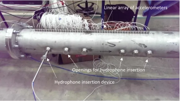
The experimental set-up used to evaluate the performance of the vibroacoustic beamforming for detecting an acoustic source into a heavy fluid is illustrated in Figure 2. For this laboratory experiment, the steam generator shell is represented by a cylindrical pipe made of stainless steel. The length, the diameter and the thickness are respectively, 3.1 m, 219 mm and 8 mm. For the ease of implementation and safety reasons, the fluid used inside the pipe is water (rather than sodium) at room temperature and at a pressure of about 4 bars. The test section is connected to the hydraulic circuit by two stiff flanges. Particular attention has been paid to decouple the test section from external mechanical sources (by fixing the pipe with rubber seals on a suspended slab) and from external fluid sources (by using acoustic decoupling balloons). Upstream the test section, a 4 m long pipe and a perforated plate flow conditioner (see figure 2c) are used to stabilize the turbulent flow whereas a 1.5m long pipe is used for the discharge before the acoustic balloon (see figure 2a).
Nine holes have been perforated on the cylindrical generator 𝜃𝑠 = 0° of the test pipe (see figure
2b). These holes are used to introduce the acoustic source inside the pipe at different axial position. The acoustic source consists in a B&K 8103 hydrophone used in transmission mode (i.e. emitter mode). The driving signal generated by a B&K PULSE system is amplified with a
B&K Power Amplifier 2713. The hydrophone is mounted on a mechanical device (see figure
2b) which has been designed for controlling the radial positions of the hydrophone.
The pipe vibrations are measured by an array of 24 KISTLER 8704B50 accelerometers fixed on the cylindrical generator 𝜃𝑖 = 90° (see figure 3). The spacing between the sensors is 𝛥𝑥 =
4 cm and the first accelerometers is positioned at 15 cm from the upstream flange of the flow. The axial position of the accelerometer #i is then 𝑥𝑖 = 0.15 + 0.04(𝑖 − 1) for 𝑖 ∈ {1, . . ,24}. The accelerometer signals have been processed using the B&K PULSE system for extracting the cross-spectral matrices, Γ. The sampling frequency and the frequency resolution have been fixed to 16384 Hz and 4 Hz, respectively. The cross-spectral matrices have been exported in order to achieve the beamforming treatments with MATLAB.
We can underline that the hydrophone is of small size compared to the diameter of the pipe and the acoustic wavelength for the considered frequency band (i.e. up to 5kHz). This characteristic ensures us that it is well adapted for simulating a monopole source. However, the counter part of this small size is the poor acoustic radiation efficiency of this projector in the considered
frequency band. Bellow 1 kHz, the signal-to-noise ratio is clearly insufficient for exploiting the results given by the accelerometers fixed on the pipe.
This experimental set-up allows us to achieve measurements for different positions of the acoustic source (i.e. hydrophone) and different flow speeds. However, for the sake of conciseness, we are going to present only the results for the highest considered flow speed. It corresponds to a flow rate of 𝑄𝑤 = 140 l. s−1.
4. Analysis of the vibroacoustic response of the test section
Before to study the performances of the vibroacoustic beamforming, one analyses the vibratory response of the test section for three different excitations:
- A radial point force applied on the pipe in order to analyse the vibroacoustic behaviour of the test section;
- An acoustic source inside the fluid to analyse the vibrations induced by the source to be detected;
- The pressure fluctuations induced by the turbulent flow to characterize the vibratory background noise measured by the array of accelerometers.
4.1 Radial mechanical point excitation
Figure 4 shows the vibratory field measured by the array of accelerometers for a radial mechanical excitation (i.e. impact hammer) applied in x = 0.14 m. The measurements have achieved when the pipe is filled with water at a pressure of 4 bars when the water is at rest. Peaks of resonances can be observed on the FRF of the accelerometer #21 (figure 4a). These ones can be attributed to two physical phenomena:
- The first one is related to the wave guide behaviour of the fluid filled pipe and its ability to exhibit propagative vibroacoustic waves in the axial direction (Fuller and Fahy 1982, Fuller 1983). For each circumferential order n of the cylindrical shell (i.e. each order of a Fourier serie decomposition of the vibratory field), one can define a cut-on frequency. For frequencies below this frequency, the waves related to this circumferential order are evanescent. They do not contribute significantly to the vibratory field on the pipe. In contrary, for frequencies above the cut-on frequency, the waves are propagative and can contribute significantly on the vibratory field. An estimation of these cut-on frequencies can be obtained by resolving the dispersion
curves of an infinite fluid loaded cylindrical shell model (Fuller and Fahy 1982, Fuller 1983). The calculation has been carried out for the present case considering a Young modulus of 1.85 × 10¹¹ Pa, a mass density of 7800 kg/m3 and a Poisson coefficient of 0.3 for steel and a
sound velocity of 1500 m/s and a mass density of 1000 kg/ m3 for water. One finds the following cut-on frequencies: 363 Hz for n=2, 1079 Hz for n=3, 2145 Hz for n=4 and 3549 Hz for n=5;
- The second phenomenon is related to the wave reflexions on the flanges. Indeed, the size of the flange section is 40 mm in the axial direction and 60 mm in the radial direction. The flanges are then significantly stiffer than the cylindrical shell. The mechanical impedance mismatch at the interface between the pipe and the flange leads to wave reflexions at both flanges. The constructive interferences of these waves for some frequencies leads to a resonance phenomenon. In the following, one names by “pseudo axial modes” these resonances. It cannot be strictly called “modes” as a part of the energy of the vibroacoustic waves can be transmitted through the fluid (i.e. water) which is not bounded in the axial direction.
These two phenomena are closely related. It results that the pseudo axial modes for a given circumferential order n occur only for frequencies above the cut-on frequency of the circumferential order. Moreover, as the celerity in the axial direction of a propagative wave is infinite at the cut-on frequency and decreases in function of the frequency (see the dispersion curves in (Fuller and Fahy 1982), it results that the density of pseudo-modes is important just above the cut-on frequency and then decreases when the frequency increases. This behaviour can be clearly observed on figure 4a. In particular, one can notice the densification of peaks around 1100 Hz and 2200 Hz which are around to the calculated cut-on frequencies for n=3 and
n=4, respectively.
The spatial distribution of the pipe vibration measured by the array of accelerometers is shown on figure 4b. For readability consideration, one has plotted the shell displacements instead of the shell accelerations. At the pseudo-mode frequencies, one can observe some patterns with pseudo nodes of vibration and antinodes. The number of antinodes is related to the axial celerity of the vibroacoustic waves. As the celerity decreases with frequency, the wavelength decreases also and then the number of antinodes increase with frequency. It should however keep in mind that several circumferential orders can contribute at a given frequency (as soon as their cut-on frequencies are below this frequency). This may explain why the pseudo-mode at 1244 Hz has 4 antinodes on the instrumented section whereas the one at 1266 Hz has only 3 antinodes. These two pseudo-modes are not related to the same circumferential order. The first one is certainly
related to n=2 whereas the second one is related to n=3. Only measurements along the circumference of the pipe would permit to confirm the circumferential order of each pseudo-mode, it is however outside the scope of the paper.
4.2 Acoustic source
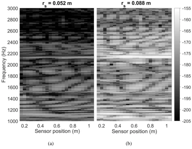
Now, let us focus on the vibratory response of the test section when it is excited by the hydrophone used in emitter mode. A sine sweep from 500 Hz to 5 kHz has been used as input signal of the amplifier of the hydrophone. Below 1 kHz, the SNR is however too low for exploiting correctly the measurements. The results will not be shown below this frequency. One plots in figure 5 the displacement results for two radial positions of the source: rs=0.052 m and rs =0.088 m, both for an axial position of xs=0.56 m corresponding around the middle of the
array.
One can notice as it can be expected that the levels are generally significantly greater when the source is closer to the steel shell (i.e. rs =0.088 m). Moreover, the patterns appearing on figure
5 are similar to those of figure 4 without to be identical. This can be explained by the fact that the acoustic source does not excite the same pseudo axial modes than the mechanical force considered in figure 4. The radial position of the source influence also the response of the pseudo axial modes. For instance, for a source located on the axis of revolution of the shell (i.e.
rs =0 m), only the pseudo axial modes corresponding to the circumferential order n=0 are
excited as the system is fully axisymmetric in this case. More the source is far the axis of revolution, more circumferential orders participate to the shell response. This can be observed on figure 5 where the peak levels are globally lower above 2300 Hz than below this frequency when rs=0.052 where they are roughly the same for all the spectrum when rs =0.088 m. This
can be explained by a lower contribution of the circumferential order n=4 for rs=0.052 than for rs =0.088 m.
Finally, one reminds that these transfer functions between the source and the accelerometers have been encapsulate in the vector noted H𝑢(𝜔) in section 2. These transfer functions will be
used for the calculation of the steering vector (with Eq. (8) for the conventional beamforming and with Eq. (11) for the MaxSNR beamforming). The array gain will also be evaluated using these transfer functions through the use of Eq. (9) for evaluating the cross-spectral matrix related to the source.
4.3 Turbulent flow
In the presence of the fluid at rest (only booster pump in operation), the signals between the different accelerometers are incoherent (result no shown). However, as it has already been observed by Moriot et al (2015), when the flow rate increases, the signals become coherent for some frequencies (see figure 10 in Moriot et al (2015)). The study of Moriot is however limited to some particular frequencies spaced of 1 kHz.
Figure 6 shows the normalized CSD function between sensor #1 and the other sensors for a flow rate of 140 l. s−s and for the frequency band [1 kHz- 3 kHz]. It can been observed that the
accelerometer signals are highly coherent for frequencies corresponding to pseudo axial modes (by comparing figure 5 with figure 3). This result was not expected at the first sight. Instead, if one considers the well-known model of Corcos (1963) of the wall pressure field induced by a turbulent boundary layer, one can calculate a coherent length of the pressure field in the stream wise direction. This one varies from 4.1 × 10⁻⁴ m (at 3 kHz) to 1.3 × 10⁻³ m (at 1 kHz). As
it is of almost one order of magnitude lower than the sensor spacing, one could expect a weak coherence of the signals of the accelerometers. Finally, it appears that it is not the case as the considered system reacts to this weakly correlated excitation. It results that the vibratory response is strongly correlated (in space) for the frequencies corresponding to pseudo axial modes. This explanation has been confirmed from numerical investigations considering an infinite shell model coupled to two ring stiffeners and excited by a homogenous established TBL excitation (Kassab 2018). This strong coherence of the vibratory field at some frequencies is clearly a drawback for the conventional beamforming which supposes the background noise uncorrelated. It is however necessary to establish the performance of this treatment in this particular condition for both, narrow band analysis and wide band analysis. This strong coherence of the background noise has also lead us to consider another type of treatment, the MaxSNR beamforming that we have introduced previously. For this treatment which is based on a prior knowledge of the background noise, one underlines that the measurements achieved for this flow rate (without the acoustic source) gives us the cross-spectral matrix of the background noise, Γ𝑛 used in Eq. (11) to estimate the steering vector.
5. Analysis of beamforming performances
In the previous section, one has analysed the accelerometer signals induced by the source to be detected (i.e. section 4.2) as well as those induced by the turbulent flow which represent the
background noise (i.e. section 4.3). These quantities are used, both, to evaluate the steering vectors and to evaluate the performance of the beamforming. We can underline that this case constitute an ideal case. Instead, in practice for the detection on the SGU, the vibrations induced by the source or those of the background noise can vary in function of the times, depending of the functional state of the installation. The values at an initial time of the quantities used for estimating the steering vectors are then not necessary representative of the values of the same quantities at the time of the detection. Here, one does not study the effect of these time variations of the signals induced by the source or of the background noise that can be due to many parameters related to the practical application.
5.1 Narrow band analysis
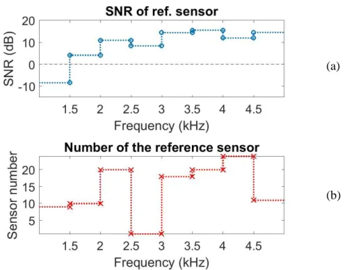
As it has been described in section 2, a pre-filtering state is defined by the reference sensor and the reference SNR. This information is given in figure 7 for an acoustic source located at (𝑥𝑠, 𝑟𝑠) = (0.56 m, 0.052 m) and a flow rate of 140 l/s. One can notice that the reference sensor
vary from one frequency to another in the studied frequency band [1 kHz-5 kHz]. It is a consequence of the variation with frequency of the spatial distribution of the vibratory field induced by the source (as shown on figure 5) as well as those induced by the turbulent flow. The SNR of reference sensor increases globally in function of the frequency. It is mainly due a decrease of the background noise with frequency. One reminds that this definition of the SNR of reference sensor is only valuable for narrow band analysis. The SNR of reference sensor for wide band analysis will be defined in section 2.
Figure 8 shows the levels of the beamforming output for the acoustic source ‘only’ (i.e. source with a very low background noise when the fluid is at rest) and for the background noise due to the turbulent at a flow rate of 140 l/s. These results have been obtained when the beamforming focus on the source using Eq. (8) with the steering vectors evaluated as described previously. Figure 8a corresponds to the conventional beamforming whereas figure 8b corresponds to the MaxSNR beamforming. The levels are expressed in dB with the same range on the two graphs. One can observe that the levels of the MaxSNR beamforming are always lower than to the conventional beamforming whatever the frequency. The differences between the two techniques appears more important for the treatment of the background noise than for the signals due to the acoustic source. This highlights the ability of the MaxSNR beamforming to reject the background noise. It results that the SNR at the beamforming output (i.e. difference of the output level with the source and with the background noise, see Eq. (6)) is generally
greater for the MaxSNR beamforming than for the conventional one. One directly compares the SNR at the beamforming output with the SNR of reference sensor by focusing on the array gain defined by Eq. (7). The result is shown on figure 9. Clearly, the gain of the MaxSNR beamforming is significantly greater than the one of the conventional beamforming whatever the frequency inside the studied frequency range. This results directly from the definition of the steering vectors of the MaxSNR beamforming which maximize the SNR at the beamforming output whereas the conventional beamforming assuming an uncorrelated background noise. The gain of the conventional beamforming exhibits significant values (i.e. 5-7 dB) at some particular frequencies but relatively low values in general. It can even be negative. These poor performances can be related to the strong coherence of the vibratory field induced by the turbulent flow as observed in figure 6 for the frequencies corresponding to the pseudo axial modes. To confirm this statement, one has evaluated the gain of the conventional beamforming using a homogeneous uncorrelated background noise instead to use the signals measured on the test section. The result has been plotted with a dotted line on figure 9. For this theoretical case, one can observe a gain varying around 9 dB, always significantly greater than the one obtained with the measured background noise. This confirms the strong negative influence of the background noise coherence on the conventional beamforming performance for the present case. For some frequencies (above 4.5 kHz for instance), these theoretical gains of the conventional beamforming may be lower than those of the MaxSNR beamforming. The use of a knowledge on the background noise permit in some situations to obtain significant gain that cannot be obtained without this knowledge even in the idealized case (i.e. uncorrelated background noise).
The analysis of the vibroacoustic behaviour of the test section in section 4 has shown the influence of pseudo-axial modes on the vibratory response of the pipe. Resonant peaks can be observed on the vibratory spectrum when the test section is excited by, either, the acoustic source to be detected or the turbulent flow inducing the background noise. In order to study the influence of these resonances on the beamforming performances, the values of the array gain for the two types of beamforming are given on Table 1 for the resonant frequencies identified from the FRF of figure 4a. These values should be compared to the values given on figure 9 for the whole frequency range. Moreover, the values corresponding to local peaks on the curves of the gain are written in bold on Table 1. One can observe that the array gain are not necessary higher or lower for the resonant frequencies compared to the other (non-resonant) frequencies. Moreover, at some resonant frequencies (for instance 1216 Hz), the curve of the gain can exhibit
a local peak whereas at some other resonant frequencies (for instance 1244 Hz), it is not the case. For one part, it can be due to the fact that the acoustic source does not excite significantly some modes compare to other ones (see figure 5a) and for another part, it may be due to the spatial coherence of the background noise that varies from one resonant frequency to another one (see figure 6).
Frequency (Hz) 1068 1096 1132 1164 1216 1244 1260 1336 1416 1512 Conv. Gain (dB) -5.1 -1.2 -4.7 -2.6 -1.1 -5.8 -3.6 -4.0 -1.2 -3.2 MaxSNR Gain (dB) 11.4 12.7 8.5 11.1 15.3 6.8 15.3 8.0 7.4 9.5 Frequency (Hz) 1616 1728 1848 1976 2112 2244 2368 2428 2496 2564 Conv. Gain (dB) -0.8 -1.8 -2.6 -8.8 -1.2 -2.7 2.1 -2.1 -0.6 0.2 MaxSNR Gain (dB) 4.4 6.8 10.7 6.6 10.1 7.8 9.4 6.1 2.8 3 Table 1. Values of the gain for resonance frequencies identified on figure 4a. Case of an acoustic source at (𝑥𝑠, 𝑟𝑠, 𝜃𝑠) = (0.56 m, 0.052 m, 0°) and for a flow rate of 140 l/s. Bold
values indicates local peaks on the curve of the gain.
5.2 Wide band analysis
In practice, the source to be detected (i.e. water-sodium reaction) is a broadband excitation (Kim et al. 2010). Then, it may be relevant to utilize all the energy induced by the source in a wide band instead to focus on one single frequency as for narrow band analysis.
A wide band analysis on a given signal consists in estimating the time-average of the square signal after filtering with a band pass filter [𝜔1, 𝜔2]. This quantities can be estimated with the ASD function of the signal and by integrating it in the frequency band [𝜔1, 𝜔2]. One can then
define the SNR in the band [𝜔1, 𝜔2] for each accelerometer i by:
SNR𝑖[𝜔1, 𝜔2]= 10log10(
∫𝜔𝜔12𝑆𝑖𝑖𝑠(𝜔)𝑑𝜔 ∫𝜔2𝑆𝑖𝑖𝑛(𝜔)𝑑𝜔
𝜔1
). (12)
The reference sensor for the band [𝜔1, 𝜔2] is defined as the sensor having the highest SNR in
this band. The SNR of the reference sensor in the band [𝜔1, 𝜔2] is then: SNRref[𝜔
1, 𝜔2] = max𝑖∈[1,𝑛][SNR𝑖[𝜔1, 𝜔2]]. (13) Figure 10 shows the values of this quantity for bands of bandwidth 500 Hz. The case presented is the same than in section 5.1. This figure can then be compared to figure 7. One can observe
that the values of SNR of the reference sensor for wide band analysis is globally lower than those of the narrow band analysis. This can be explained by the fact that the reference sensor change from one frequency to another for narrow band analysis (as seen in figure 7a) whereas a single reference sensor is attributed to all the frequencies contained in the frequency band for wide band analysis.
The beamforming output level for the band [𝜔1, 𝜔2] is deduced from numerical integration of the frequency-dependant output 𝑦𝑢(𝜔) over the frequency band [𝜔1, 𝜔2]. One can then evaluate
the SNR at the beamforming output and the array gain for the band [𝜔1, 𝜔2].
Figure 11 shows the array gain obtained for bands of 500 Hz bandwidth. The array gain of the conventional beamforming remains below 5 dB (excepted for the band [2 kHz-2.5 kHz]). It appears that this treatment is inefficient for these flow conditions. In the rest of the paper, one will focus on the MaxSNR beamforming performance. For this treatment, the array gain is significant with variations between 9 dB and 23 dB. These values appear globally higher than those observed in narrow bands. This can be attributed for one part, to the difference of pre-filtering reference between the two analysis (as it has been pointed previously by comparing the SNR of the reference sensor of figures 7 and 10) and for another part, to the integration in the frequency band of the beamforming output.
Figure 12 allow us studying the variations of the gain in function of the source positions. When the source is axially positioned at the middle of the array (i.e. 𝑥𝑠 = 0.56 m), one notices that the gain is generally greater for 𝑟𝑠 = 0.088 m than for 𝑟𝑠 = 0.052 m. Compared to the last, the first position is closer to the wall of the cylindrical shell. As we have discussed in section 4.2, the vibratory levels are higher for 𝑟𝑠 = 0.088 m than for 𝑟𝑠 = 0.052 m (see figure 5). However, this should not influence the array gain as it expresses an increase of SNR compared to the SNR of the reference sensor. It is most likely due to the fact that for frequencies above 2.3 kHz, the circumferential order n=4 is less predominant for rs=0.052 than for rs =0.088 m (as discussed
in section 4.2) whereas it remains significant for the background noise (see figure 6). This could explain the lower gain for rs=0.052 than for rs =0.088 for frequency bands above 2 kHz.
On another hand, when the source is not located in the front of the array gain (i.e. for 𝑥𝑠 =
1.56 m or for 𝑥𝑠 = 2.06 m), one observes that the gain is generally slightly lower compared to
the case 𝑥𝑠 = 0.56 m. It remains however significant. This shows that the MaxSNR beamforming can be efficient even if the source is not in the front of the array.
The beamforming output levels in the detection space 𝜃 = 0° are shown on Figure 13 for the 4 source positions. These results corresponds to the frequency band [4.5 kHz-5 kHz]. As the measurements have been achieved for only 9 positions, white cross indicate the positions that are not available. Figure 13a shows the output levels induced by the background noise (i.e. without the source to be detected). It is almost uniform around -43dB. The output levels in presence of the source are shown on Figure 13b-d for the four position. The real location of the source is symbolised by a black spot. In opposition to the conventional beamforming, the steering vectors of the MaxSNR are not defined such that the beamforming output is maximum when the beamforming focus on the effective position of the source. One can however observe that the output level is always the highest in the detection space for the real position of the source. For the present case, it appears that the MaxSNR beamforming is able to localize the source. This figure allows us highlighting the interest of the beamforming for increasing the SNR. Indeed, the SNR of the reference sensor are respectively, 14, 16, 17 and 11 dB for the positions of figure 13b-d. On figure 13b for instance, the maximum output level of MaxSNR beamforming is -7 dB whereas the output with only background noise is at -43 dB (see figure 13a). The difference of 36 dB between a state without the source and with the source is 22 dB greater than the SNR of the reference sensor (i.e. 14 dB). This exceeding of level (that correspond to the array gain) can be used to detect the source minimizing the false alarm.
6. Conclusions
The works presented in this paper have occurred in the framework of the development of a non-intrusive monitoring technique for the detection of a sodium-water reaction in the steam generator unit of a liquid sodium fast reactor. The technique is based on vibratory measurements on the external shell of the steam generator unit. The vibroacoustic beamforming can be used to increase the SNR in order to detect the signal due to the source when it can be embedded in the background noise. The study was conducted on a pipe test section where the source to be detected consisted on a hydrophone used in emitter mode placed inside the pipe while the disturbing noise is induced by the water turbulent flow. A linear array composed of 25 accelerometers fixed on the pipe was used for the vibratory measurement. The efficiencies of the conventional and the MaxSNR beamformings have been studied.
The conventional beamforming has appeared inoperative at significant flow rates (i.e. 140 l. s−1) in the considered band [1 kHz - 5 kHz]. This results of the strong coherences of the
vibratory signals induced by the turbulent flow which are in contradiction with the assumption made by the conventional beamforming. On the other hand, significant gains (around 10 to 25 dB) have been observed using the MaxSNR beamforming for different positions of the source which are not necessary in the front of the array. An analysis on the beamforming output in the detection has also shown that it can be used for the localisation of the source for the considered case.
It should nevertheless be noted that these gains results from considering “ideal” data to define the steering vectors:
- the source-sensor transfer functions considered were measured on the pipe;
- the cross-spectral matrix of accelerations characterizing the noise has been used both to define the steering vectors and to evaluate the array gain.
In the future, it will be necessary to develop a reliable vibroacoustic model of the considered system to predict the source-sensor transfer functions as it may be difficult to measure them for the practical application. Moreover, a sensitivity analysis of the variations of the background noise on the beamforming performance should be achieved. Finally, it must be recalled that the majority of background noise in an operating steam generator is due to the combined noise of sodium flow and water evaporation, while we only assimilated it to turbulent flows. Only more representative experiments could confirm the interest of the vibroacoustic beamforming considering the MaxSNR treatment for the detection of the sodium-water reaction in a SGU.
REFERENCES
Cavaro, M., Payan, C., Jeannot, J.P., 2013. Towards the bubble presence characterization within the SFR liquid sodium, In: Proceedings of ANIMMA International Conference, Marseille, France, vol. 1127, June.
Chikazawa, Y., 2010. Acoustic leak detection system for sodium-cooled reactorsteam generators using delay-and-sum beamformer. J. Nucl. Sci. Technol. 47(1), 103–110.
Chikazawa, Y., Yoshiuji, T., 2015. Water experiment on phased array acoustic leak detection system for sodium-heated steam generator. Nucl. Eng. Des. 289, 1-7.
Corcos G.M., 1963. The resolution of pressure in turbulence, J. Acoust. Soc. Am. 35, 192-199.
Fuller, C. R., Fahy, F. J., 1982. Characteristics of wave propagation and energy distributions in cylindrical elastic shells filled with fluid. J. Sound Vib. 81 (4), 501–518.
Fuller, C. R., 1983. The input mobility of an infinite circular cylindrical elastic shell filled with fluid. J. Sound Vib. 87 (3), 409-427.
Hayashi, K., Shinohara, Y., Watanabe, K., 1996. Acoustic detection of in-sodium water leaks using twice squaring method. Ann. Nucl. Energy 23, 1249-1259.
Kim, T., Yugay, V. S., Jeong, J., Kim, J., Kim, B., Lee, T., Lee, Y., Kim, Y., Hahn D., 2010. Acoustic Leak Detection Technology for Water/Steam Small Leaks and Microleaks Into Sodium to Protect an SFR Steam Generator. Nucl. Technol. 170, 360-369.
Kassab, S., 2018. Vibroacoustic beamforming for the detection of an acoustic monopole inside a thin cylindrical shell coupled to a heavy fluid: Numerical and experimental developments, PhD thesis, Université de Lyon, INSA Lyon, Villeurbanne, France, 182 p. (in French).
Moriot, J., Maxit, L., Guyader, J.L., 2012. Detection and localization of a leak in a sodium fact reactor steam generator by vibration measurements. In: Proceedings of Euronoise, Prague, Czech Republic, June.
Moriot, J., 2013. Passive vibroacoustic detection of a water-sodium reaction using beamforming on a steam generator of a liquid sodium fast reactor, PhD thesis, INSA Lyon, France, 158 p. (in French).
Moriot, J., Maxit, L., Guyader, J.L., Gastaldi, O., Périsse, J., 2015. Use of beamforming for detecting an acoustic source inside a cylindrical shell filled with a heavy fluid. Mech. Syst. Signal Process 52–53, 645–662.
Singh, R.K., Rao, A.R., 2011. Steam Leak Detection in Advance Reactors via Acoustics method. Nucl. Eng. Des. 241, 2448–2454.
Tanaka, T., Shiono, M., 2014. Acoustic Beamforming with Maximum SNR Criterion and Efficient Generalized Eigenvector Tracking. In: Proceeding of the 15th Pacific-Rim Conference on Advances in Multimedia Information Processing, Malaysia, December. Van Veen, B., Buckley, K., 1988. Beamforming: a versatile approach to spatial filtering. IEEE ASSP magazine 5 (2), 4-24.
Figure 1.Schematic representation of the configuration considered for assessing the performance of the vibroacoustic beamforming.
(a)
(b)
(c)
Figure 2. Experimental setup schemes: (a), Pipe test section inserted in the hydraulic loop; (b), Pipe test section with the various holes for the hydrophone insertion; (c), Hydrophone
mounting system (left) and perforated plate conditioner (right).
x r θ Openings for hydrophone insertion Acoustic decoupling tank Test section
Perforated plate flow conditioner Downstream stabilization section Acoustic decoupling tank Upstream discharge section Water tank Pump Hydrophone insertion device
Figure 3. Picture of the test pipe with the linear array of accelerometers.
Linear array of accelerometers
Hydrophone insertion device
(a)
(b)
Figure 4. Radial displacement response of the test pipe for an unit radial mechanical point force at x=0.105 m (hammer excitation): (a), Frequency Response Function (FRF) at point x=1 m (i.e. sensor #21); (b), Displacement versus sensor position and frequency (dB, ref. 1
(a) (b)
Figure 5. Radial displacement response in function of the sensor position and the frequency (dB, ref. 1 m) for an acoustic source excitation (i.e. hydrophone emitter) at two positions:
Figure 6. Normalized cross spectrum density function between sensor #1 and sensor #i. Results in function of the position of sensor #i and the frequency for a flow rate of 140 l/s.
(a)
(b)
Figure 7. (a) Signal to noise ratio for the reference sensor. (b), number of the reference sensor for each frequency. Case of an acoustic source at (𝑥𝑠, 𝑟𝑠, 𝜃𝑠) = (0.56 m, 0.052 m, 0°) and for
(a) (b)
Figure 8. Output levels of the beamforming focusing on the source in presence of the source only (full) and for the noise only (dash): (a), Conventional BF; (b), MaxSNR BF. Case of an
Figure 9. Array gain in function of the frequency: full, MaxSNR BF; dash, conventional BF; dash; dotted, theoretical values for the conventional BF supposing uncorrelated noise. Case of
(a)
(b)
Figure 12. Gain with the MaxSNR beamforming for different source positions: full, (𝑥𝑠, 𝑟𝑠) = (0.56 m, 0.052 m); dash, (𝑥𝑠, 𝑟𝑠) = (0.56 m, 0.088 m); dash-dotted, (𝑥𝑠, 𝑟𝑠) =
(2.06 m, 0.052 m); dotted, (𝑥𝑠, 𝑟𝑠) = (1.56 m, 0.088 m). Wide band analysis of 500 Hz bandwidth.
(a) (b) (c) (d) (e)
Figure 13. Level (dB) of the MaxSNR beamforming output for different steering positons. Five configurations with a flow rate of 140 l/s: (a), only the background noise; (b), source at
(𝑥𝑠, 𝑟𝑠) = (0.56 m, 0.052 m); (c), source at (𝑥𝑠, 𝑟𝑠) = (0.56 m, 0.088 m); (d), source at,(𝑥𝑠, 𝑟𝑠) = (2.06 m, 0.052 m); (e), source at (𝑥𝑠, 𝑟𝑠) = (1.56 m, 0.088 m). Results for the
band [4.5 kHz-5 kHz]. Position of the source symbolized by a black disk. Unavailable position symbolized by a white cross.