HAL Id: hal-03117133
https://hal.archives-ouvertes.fr/hal-03117133
Submitted on 21 Jan 2021
HAL is a multi-disciplinary open access
archive for the deposit and dissemination of
sci-entific research documents, whether they are
pub-lished or not. The documents may come from
teaching and research institutions in France or
abroad, or from public or private research centers.
L’archive ouverte pluridisciplinaire HAL, est
destinée au dépôt et à la diffusion de documents
scientifiques de niveau recherche, publiés ou non,
émanant des établissements d’enseignement et de
recherche français ou étrangers, des laboratoires
publics ou privés.
Brown cruise using measurements of nonmethane
hydrocarbons, CH 4 , CO 2 , CO, 14 CO, and δ 18
O(CO)
Jens Mühle, Andreas Zahn, Carl A. M. Brenninkmeijer, Valérie Gros, Paul J.
Crutzen
To cite this version:
Jens Mühle, Andreas Zahn, Carl A. M. Brenninkmeijer, Valérie Gros, Paul J. Crutzen. Air mass
classification during the INDOEX R/V Ronald Brown cruise using measurements of nonmethane
hydrocarbons, CH 4 , CO 2 , CO, 14 CO, and δ 18 O(CO). Journal of Geophysical Research, American
Geophysical Union, 2002, 107 (D19), �10.1029/2001JD000730�. �hal-03117133�
Air mass classification during the INDOEX R/V
Ronald Brown cruise using measurements
of nonmethane hydrocarbons, CH
4, CO
2,
CO,
14CO, and
␦
18O(CO)
Jens Mu¨hle, Andreas Zahn, Carl A. M. Brenninkmeijer,
Vale´rie Gros, and Paul J. Crutzen
Air Chemistry Division, Max Planck Institute for Chemistry, Mainz, Germany
Received 6 October 2000; revised 7 March 2001; accepted 2 April 2001; published 6 September 2002.
[
1] During the Indian Ocean Experiment (INDOEX) in February-March 1999 the impact
of continental outflow to the Indian Ocean was analyzed. On board the R/V Ronald
Brown altogether 93 air samples were taken for analysis of nonmethane hydrocarbons
(NMHC), methane (CH
4), carbon dioxide (CO
2), carbon monoxide (CO), and the
14C/
12C
and
18O/
16O isotope ratios of CO. Five types of air masses differing in origin, degree of
pollution, and chemical age were identified based on back trajectory analyses and the
trace gas data, supported by continuous CO and ozone (O
3) observations from other
investigators. The Indian Ocean was found to be frequently affected by nearby emissions
from the Indian subcontinent and Indochina, but the strongest pollution event
(characterized inter alia by high mixing ratios of medium- and long-lived NMHC) was due
to long-range advection from the extratropical northern hemisphere. Carbon monoxide 14
showing a distinct meridional profile unequivocally confirms this remote impact. The ratio
acetylene/CO was found to be often inadequate as a measure for atmospheric processing,
the integrated influence of OH chemistry and mixing. Our data suggest that the influence
from fresh continental pollution was less pronounced along the INDOEX R/V Ronald
Brown cruise compared to observations made during other tropical campaigns, such as the
Pacific Exploratory Mission-West B in the Pacific Ocean.
INDEXTERMS: 9340 InformationRelated to Geographic Region: Indian Ocean; 0368 Atmospheric Composition and Structure: Troposphere— constituent transport and chemistry; 1040 Geochemistry: Isotopic composition/chemistry; 3307 Meteorology and Atmospheric Dynamics: Boundary layer processes; 3374 Meteorology and Atmospheric Dynamics: Tropical meteorology; KEYWORDS: INDOEX, Indian Ocean, NMHC, isotopes, air mass classification, long-range
transport
Citation:Mu¨hle, J., A. Zahn, C. A. M. Brenninkmeijer, V. Gros, and P. J. Crutzen, Air mass classification during the INDOEX R/V Ronald
Brown cruise using measurements of nonmethane hydrocarbons, CH4, CO2, CO,14CO, and␦18O(CO), J. Geophys. Res., 107(D19), 8021, doi: 10.1029/2001JD000730, 2002.
1. Introduction
[2] The fast industrialization of countries in Asia, in
par-ticular India and China, comes along with large and rapidly increasing emissions of various pollutants to the atmosphere. Especially during the winter (northeast) monsoon (January-March), the Indian Ocean becomes a unique region where the temporal and spatial development of emissions from the In-dian subcontinent and Southeast Asia can be studied. This particularly implies the mixing of continental outflow of pol-lutants and aerosols with pristine SH air masses by cross-equatorial monsoonal flow into the Intertropical Convergence Zone (ITCZ). A major intention of the Indian Ocean Exper-iment (INDOEX) was to improve the understanding of the interactions between aerosols, clouds, chemistry, and climate. Special emphasis was on the radiative forcing effect of anthro-pogogenic aerosols and on the role of the ITCZ in
interhemi-spheric transport of trace gases and aerosols. The intensive field campaign of INDOEX took place in February-March 1999 and involved several aircrafts, ships, and island stations in the Indian Ocean region. A main goal of the National Oceanic and Atmospheric Administration (NOAA) research vessel
Ro-nald Brown as one of the platforms was to characterize the
trace gas and aerosol composition of outflow from the Indian subcontinent and its chemical processing over the Indian Ocean.
[3] Prior to INDOEX, only sparse trace gas observations
have been carried out in the Indian Ocean such as the second Soviet American Gases and Aerosols campaign (SAGA II) in 1987 [Butler et al., 1988; Arlander et al., 1990; Johnson et al., 1990] or the Joint Global Ocean Flux Study (JGOFS) during which nitrous oxide (N2O), CH4, and CO2 were measured
[Bange et al., 1996, 1998; Goyet et al., 1998; Upstill-Goddard et
al., 1999, and references therein]. More recent studies in this
region (predominantly on tropospheric O3) [Baldy et al., 1996;
Gros et al., 1998; de Laat et al., 1999; Taupin et al., 1999] point
to considerable impact of continental pollutants, even at very Copyright 2002 by the American Geophysical Union.
Paper number 2001JD000730. 0148-0227/02/2001JD000730
remote stations. This finding was confirmed by shipborne trace gas and aerosol measurements in 1995 by Rhoads et al. [1997], as part of the World Ocean Circulation Experiment (WOCE), as well as by CO, CH4, O3, and aerosol measurements by Lal
et al. [1998]. A compilation of further pre-INDOEX research
can be found in the works of Rhoads et al. [1997] and Mitra [1999], and at http://www-indoex.ucsd.edu/databyevent.html. Besides these campaigns, the NOAA/Climate Monitoring and Diagnostics Laboratory (CMDL) monitors CO, CH4, and CO2
at several stations in the Indian Ocean [Novelli et al., 1995, 1998].
[4] Purpose of the present paper is to characterize the air
masses encountered by the R/V Ronald Brown by applying a powerful set of contrasting tracers, in particular nonmethane hydrocarbons. The detected trace gases (NMHC, CH4, CO,
CO2, N2O, and SF6) do have lifetimes between days (e.g.,
propane) and years (e.g., CH4) and diverse sources, e.g.,
bio-genic, oceanic, and anthropogenic (see Table 1).
[5] Although NMHC play a key role in atmospheric
chem-istry, particularly with respect to photochemical O3
produc-tion, only little information is available on their fate in the Indian Ocean area, especially during the INDOEX conditions, i.e., the northern Indian Ocean during the winter monsoon. General information on the global distribution and seasonality of NMHC and their fate in the atmosphere is given by Singh
and Zimmerman [1992] and Rudolph [1995] (additional details
are given by Rudolph et al. [1996] and Bonsang and Boissard [1999]). Even pristine areas of the southern hemisphere (SH) are influenced by long-range transport of long-lived NMHC emitted by continental sources [e.g., Touaty et al., 1996; Saito et
al., 2000], while short-lived NMHC are determined by
emis-sions from the ocean [e.g., Bonsang et al., 1993; Plass-Du¨lmer et
al., 1995; Lewis et al., 1999].
[6] In addition to the mixing ratio of CO, its C18O (stable)
and 14CO (radioactive) isotope composition was measured.
␦18O(CO) expresses the isotope ratio18O/16O in CO relative
to the Vienna-Standard Mean Ocean Water (V-SMOW) stan-dard in per mil. High␦18O(CO) values (⬃23‰) are associated
with fossil fuel combustion, whereas biomass burning derived CO is less enriched (15 to 18‰), and photochemically gener-ated CO is assumed to show ␦18O(CO) of ⬃0‰. Note that
isotope fractionation during oxidation by OH yields progres-sive depletion in␦18O(CO). Atmospheric14CO (given in
mol-ecules per cm3 air STP) is mainly produced by cosmic rays,
primarily in the midlatitude and high-latitude upper tropo-sphere and lower stratotropo-sphere. It has also a small biogenic contribution (“recycled CO”) from the incomplete oxidation of organic matter containing 14C from CO
2 assimilation. The
main sink of14CO is, as for CO, oxidation by OH. Note, that
CO from fossil fuel combustion is free of 14CO. Observed
isotopic composition of CO thus reflects both the signature of the different sources as well as fractionation and dilution oc-curred during transport [Brenninkmeijer et al., 1999; Jo¨ckel, 2000, and references therein].
[7] After a brief description about the analytical techniques
applied (section 2), a short overview about the meteorological conditions during INDEX is given (section 3). Thereafter the observed trace gas time series are analyzed (section 4), and the intersected air masses are classified based upon back trajectory analyses and the trace gas data (section 4.1). The influence of long-range transport on the observed trace gas variability is discussed (section 4.2), and the meaning of the acetylene/CO ratio is evaluated (section 4.3). Finally, the entire data set is compared with previous results (section 5), and the conclusions are given (section 6).
2. Experimental Techniques
2.1. Air Sampling and Analyzed Compounds
[8] Ninety-three air samples (sample locations in Figure 1)
were collected in 2.5 L electropolished stainless steel canisters fitted with metal bellow valves (Nupro SS-4H). Using a metal bellows pump (Parker, MB-158-E, operation temperature be-low 65⬚C), air was sucked from the top of a bow tower (10 m height) via a 25 m stainless steel tube (ID: 4 mm) through an ice water cold trap (0⬚C) to reduce the water vapor mixing ratio to⬃0.6%. After flushing several times, the canisters were filled to a final pressure of 3.7 bar leading to sample sizes of⬃9 L (STP) each. With exception of the transport time (⬃6 days) to the laboratory (MPI-C, Mainz, Germany) the canisters were kept at ⫺18⬚C. Twelve hours before gas chromatographic (GC) analysis of NMHC, CH4, CO2, SF6, and N2O the
canis-ters were stored at ambient temperature.
[9] For measuring CO and its isotope ratios (18O/16O,14C/
12C), fifteen 600 L (STP) air samples (sample locations in
Figure 1) were also collected from the bow tower (via a1⁄2inch
Table 1. Rate Constants and Lifetimes of Selected Trace Gases Under Typical Midlatitude and Tropical Conditions
Compound Main Sources cmK3OHmoleculeat 298 K,⫺1s⫺1
OH Photochemical Lifetimes, days [OH]midlatitudes, 5⫻ 105 molecule cm⫺3 [OH]tropics, 3⫻ 106 molecule cm⫺3 Methanea, b industrial/natural gas loss/wetlands/
ruminants/biomass burning 6.34⫻ 10
⫺15c 3650 (10 years) 608 (1.7 years)
Ethanea, d natural gas loss/biomass burning/ 2.40⫻ 10⫺13c 96.5 16.1
Propanea vegetation 1.09⫻ 10⫺12c 21.2 3.5
Acetylenea industrial/biomass burning 7.47⫻ 10⫺13c 31.0e(30.3f) 5.2e(5.2f)
Carbon monoxidea, b industrial/biomass
burning/hydrocarbons⫹ OH (1.5⫹ 0.9 Patm)⫻ 10 ⫺13c 96.5(1 atm) 16.1(1 atm) a[Hough, 1991]. b[IPCC, 1995]. c[DeMore et al., 1997]. d[Rudolph, 1995]. eHere 25 ppb O 3. fHere 30 ppb O 3.
PFA tube) by using 5 L aluminum cylinders (Scott-Marrin Inc., Riverside California). An improved version of the clean air compressor described by Mak and Brenninkmeijer [1994] was used. The flushing and filling procedure took⬃60 min.
[10] On the samples collected during the pre-INDOEX leg 0 (12–19 February 1999, day of year (DOY) 43–50) and INDOEX leg 1 (22–28 February 1999, DOY 53–59), analysis of CH4, CO (including its isotopic composition), CO2, N2O,
and SF6 were performed. For leg 2 (5–22 March 1999, DOY
64–81) and leg 3 (26–30 March 1999, DOY 85–89), addition-ally NMHC were analyzed. Owing to the limited additional information derived, the N2O and SF6data are not assessed in
detail.
2.2. Laboratory-Based NMHC Measurements
[11] A general overview about gas chromatographic
tech-niques for measuring atmospheric trace species is given by
Camel and Caude [1995] and Helmig [1999]. Here the 59
sam-ples from leg 2 and 3 were separated on a 50 m, ID: 0.32 mm, 5 m Al2O3/KCl porous layer open tubular (PLOT) column
(Chrompack) by using a gas chromatograph (Hewlett-Packard, HP 6890) with subambient temperature capability connected to a quadrupole mass spectrometer (HP 5973). Sample ali-quots of 350 ml (STP) air initially passed two scavenger traps (length: 11 cm, ID: 0.7 cm) filled with anhydrous lithium hy-droxide (Merck) and anhydrous magnesium perchlorate (Fluka) to remove CO2and H2O. Tests indicated insignificant
influence of the scavenger traps on the measured NMHC
[Ma-tusˇka et al., 1986; Habram et al., 1998; Kurdziel, 1998; Rasmus-sen et al., 1996; Lewis et al., 1999]. The condensible compounds
(encompassing the NMHC) were cryogenically concentrated in a stainless steel microtrap (⫺170⬚C, length: 30 cm, ID: 0.03 inch), packed along 10 cm with porous silica beads (Unibeads 1S, 60/80 mesh, Alltech) over 8 min at a flow of 45 mL min⫺1
(controlled by a mass flow controller, MKS Type 1179A). Sim-ilar techniques were used by Singh et al. [1988], Rudolph et al. [1990], Doskey [1991], Doskey et al. [1992], and Mitra and Yun [1993]. During trapping, the sample trap was connected to an evacuated gas reservoir (2.54 L) to determine the sample size volumetrically. Afterwards, the trap was flushed with helium for 5 min to remove traces of oxygen and nitrogen.
[12] The retained compounds were desorbed from the trap
by heating from the initial⫺170⬚C to ⫹150⬚C in ⬃3 s [Mitra
and Yun, 1993] and introduced into the analytical column. The
GC column was held at 10⬚C for 11 min and subsequently heated at 5⬚C min⫺1 to 200⬚C and maintained at 200⬚C for
another 10 min. Helium 6.0 further purified by a three-stage gas purifier and a cryogenic trap (filled with activated charcoal) at liquid nitrogen temperature was used as carrier and flushing gas. The initial column head gauge pressure was 0.81 bar at 10⬚C, increased during heat up of the column to maintain a constant flow. All connections were made of compression type stainless steel fittings. The sample path and the inlet line are of stainless steel and silcosteel (Restek Corp.), respectively, held at 60⬚C to avoid condensation of species of low vapor pressure. [13] The mass spectrometric detector was operated in
Single-Ion Monitoring (SIM) mode to enhance sensitivity com-pared to SCAN mode. For each compound, m/z values were carefully chosen with respect to background, coeluting pounds and sensitivity. One characteristic m/z value per com-pound was used to derive its concentration, and up to three other m/z values were used to check identity and to cross-check correct quantification for the (unlikely) case of coelution. Most of the analyzed compounds were clearly separated, except of acetylene (C2H2) and butane. Each chromatogram was
inte-grated by a MSD Software (Hewlett-Packard) and checked manually. The mass spectrometer was tuned weekly. Analyses have been made for light alkanes such as ethane (27), propane (29), butane (43), iso-butane (43), pentane (43), iso-pentane (43), light alkenes such as ethene (27), propene (41), 1-butene (41), trans-2-butene (41), cis-2-butene (41), and acetylene (26); the m/z values used for quantification are in parenthesis.
[14] A calibration following each fourth sample was made
by aliquoting different volumes of a standard gas mixture (1 to 10 mL) leading in a linear calibration line (r2ⱖ 0.99) for each
compound. The detection limits (3 variation of a blank sam-ple) were 0.2 to 6.8 pptv (ethane, propane, butane, iso-butane, pentane, and iso-pentane), 0.2 to 16.1 pptv (ethene, propene, 1-butene, trans-2-butene, cis-2-butene), and 14 to 26 pptv (acetylene), and the precision was 5 to 10%.
[15] A 30 compound reference standard from the National
Figure 1. Cruise track of the R/V Ronald Brown during IN-DOEX (11 February to 30 March 1999, day of year (DOY) 42–89), showing the locations of 9 L (STP) air samples (open symbols) and 600 L air samples for isotopic analyses of CO (solid circles, labeled 1–9 and 11–16). DOY are noted as small numbers. The four typical airflows over the Indian Ocean are labeled as F1, F2, F3, and F4, and the positions of the strong
convergence zones are marked with ITCZ (see section 3). For a better visualization, leg 1 (open circles, 22–28 February, DOY 53–59), leg 2a (open squares, 5–15 March, DOY 64–74), leg 2b (open squares, 16–22 March, DOY 78–81), and leg 3 (open triangles, 26–30 March DOY 85–89) are shown in the top part, and leg 0 (open diamonds, 12–19 February, DOY 43–50) is shown in the lower part. For legs 0 and 1, CH4, CO2,
N2O, SF6, and isotopic composition of CO were analyzed. For
Physical Laboratory (Teddington, United Kingdom) with a certified uncertainty range of 1.2 to 2.2% (95% confidence limit) for each compounds was used for absolute calibration. The calibration is currently cross-checked by measuring sam-ples used during the Nonmethane Hydrocarbon Intercompari-son Experiment (NOMHICE) [Apel and Calvert, 1994; Apel et
al., 1994, 1999]. First comparisons show an agreement within
⬃20% for all species addressed in this paper.
[16] Long-term laboratory tests (11 months) have revealed
significant formation of alkenes in the sample canisters, a prob-lem already discussed by Donahue and Prinn [1993]. Even in sample canisters kept at⫺18⬚C we detected production rates of⬃4 ppt month⫺1for ethene and⬃2 ppt month⫺1for
pro-pene. No significant changes for alkanes and acetylene were noticed. However, it is worth mentioning that the measured ethene (28 to 128 ppt) and propene (10 to 50 ppt) mixing ratios were highly correlated. This ethene to propene slope of 2.7 ppt/ppt (r2⫽ 0.90) stands in agreement with values determined
by on-line measurements on the Atlantic Ocean of 2.5 in the SH and 2.9 in the NH [Rudolph and Johnen, 1990]. As we are not able to precisely determine how much the INDOEX alk-ene data were affected by storage artifacts, they are not further discussed.
2.3. Measurement of Long-lived Trace Gases, CO, ␦18O(CO), and14CO
[17] Analyses of CH4, CO2, N2O, and SF6were made with
an automated GC system (Hewlett Packard, HP 6890a) with flame ionization detector (FID), electron capture detector (ECD), and a HP 5790 nickel catalyst for reduction of CO2to
CH4(set up by Atmospheric Environmental Service, Canada)
[Bra¨unlich, 2000]. The absolute uncertainty of the measure-ments is 3 ppb for CH4, 0.3 ppm for CO2, 2 ppb for N2O, and
0.1 ppt for SF6. CH4, CO2, and N2O are given versus the
NOAA scale, SF6is calibrated on a GC system, described by
Maiss et al. [1996].
[18] The 600 L (STP) samples are analyzed for the
concen-tration of CO and its isotopic composition (␦18O(CO),14CO).
The CO concentration is derived with an absolute measure-ment method, based on the conversion of CO into CO2and
subsequent volumetric measurement of the derived CO2. The 18O/16O isotope ratio of CO is determined by mass
spectrom-etry, and the 14C content is analyzed via accelerator mass
spectrometry [see Brenninkmeijer, 1993; Brenninkmeijer et al., 1999, 2001].
[19] The continuous measurements of CO and O3[Stehr et
al., 2002] were done with a TECO 48 CO and a TECO 49 O3
analyzer (Thermo Environmental Instruments Inc., Franklin, Massachusetts), respectively, here given as 30 min averages. The agreement between continuous CO and laboratory based CO measurements on the 600 L samples is generally better than 5 ppb.
3. Meteorology During INDOEX
[20] A short overview about the meteorological conditions
encountered along the ship track and the major near-surface airflows over the Indian Ocean is given here.
3.1. Dominating Airflows
[21] A 10 year climatological study of the Indian Ocean
presented in the meteorology overview by Verver et al. [2001] pointed out that four prevailing airflows (F1, F2, F3, F4) advect
(mainly continental) air to the Indian Ocean (Figure 1): F1,
northeast (NE) trades over the western Arabian Sea, F2,
NE-NW flow along the west coast of India, F3, NE trades over
the west Bay of Bengal, and F4, NE flow from Southeast Asia.
They are mainly driven by pressure difference developing be-tween subtropical high-pressure systems stretched along 20⬚N (from Arabia to Southeast Asia) and organized clusters of convective systems around the equator (15⬚S to 10⬚N). The strength of the four airflows fluctuates on a day-to-day basis, strongly modulated by the actual weather regime.
[22] During INDOEX, F1 was generally the most active
channel, but it was west of the region examined and thus was never passed by the Ronald Brown. F3was very active up to 6
March (DOY 65) and was most likely responsible for the polluted air masses probed at⫾2⬚N, 70⬚E during the end of leg 1 (27–28 February, DOY 58–59) and at 5–6⬚N, 70–73⬚E the beginning of leg 2a (5–6, March, DOY 64–65). Exceptionally, during the major part of leg 2 (7–22 March, DOY 66–81) and the entire leg 3 (26–30 March, DOY 85–89) the two eastern channels F3and F4were nearly absent, but channel F2was (in
contrast to February) quite active. These anomalies had crucial consequences for the trace gas composition probed during leg 2 and 3: (1) during 9–16 March (DOY 68–75), F2 brought
midlatitude air (from 20⬚–45⬚N) to the measurement site at 2⬚–19⬚N, 68⬚–75⬚E (Arabian Sea), and (2) during leg 3 (taken place in the Bay of Bengal) polluted but aged continental air (earlier imported by F3and F4) was intersected.
3.2. Location of the Intertropical Convergence Zone (ITCZ)
[23] In February-March 1999 the ITCZ was broken into
two convergence zones (CZ) [Verver et al., 2001]. The northern CZ was more active in February at 1⬚S–7⬚N, and the southern CZ became dominant in March between 10⬚S, 60⬚E and 5⬚S, 100⬚E, along the region of highest sea surface temperatures of 28⬚–29⬚C. The transition zone between SH air and NH air, unambiguously identified by a sharp jump in several trace species, such as CO from ⱕ65 ppb (SH) to ⱖ95 ppb (NH), coincided with the northern CZ on 26 February (end of DOY 57) at⬃1⬚S and with the southern CZ encountered on 19–20 March (DOY 78–79) south of 9⬚S (Figure 1).
4. Results and Discussion
[24] As seen in Figure 1, the 93 sample locations are quite
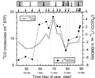
homogeneously distributed over the various legs with an aver-age sample frequency of 2.3 canisters (9 L STP) per day. The time series of medium- and longer-lived trace gases show sub-stantial variability (Figure 2). The highest concentrations were observed on 10 March (DOY 69), except for CO that peaked on 6 March (DOY 64.9). All trace gases minimized during 19–20 March (DOY 78–79) as the ship was south of the chem-ical ITCZ. These trace gas changes are expected to reflect predominantly the different origin of the air masses since the transport timescale (about 1 week) is shorter than the chemical lifetime for most of the shown trace gases. To support this claim, back trajectories were calculated, and the inferred air mass classification was subsequently compared with the trace gas signature observed in the different types of air masses. 4.1. Trajectory and Trace Gas Composition
Based Air Mass Classification
[25] For each individual sampling location, diabatic 3-D
with the Hybrid Single-Particle Langrangian Integrated Tra-jectories (HYSPLIT) program [Draxler and Hess, 1998] to es-timate the origin of the probed air masses. On the basis of the air mass classification proposed by Rhoads et al. [1997] and further specified by altogether five types of W. P. Ball et al. (unpublished manuscript, 2002), air masses were encountered during the INDOEX R/V Ronald Brown cruise. During legs 2 and 3, four air mass types were intersected: Northern Hemi-sphere continental tropical (NHcT), Northern HemiHemi-sphere continental extratropical (NHcX), Northern Hemisphere ma-rine tropical (NHmT), and Southern Hemisphere mama-rine trop-ical (SHmT). During legs 0 and 1, also Southern Hemisphere maritime extratropical (SHmX) air was temporarily inter-cepted. The identification of the individual types of air masses was done with respect to the starting area of the back trajec-tories by applying the following rules:
[26] NHcX air parcels originated from the continental
ex-tratropics (mainly from Arabian Peninsula, Middle East, and Europe) and were advected to the sampling site via the airflow F2 south-eastward along the coast of Pakistan and
the Indian west coast. Trajectories that started over the Indian subcontinent were attributed to NHcT air. They reached the Indian Ocean mostly via F3(e.g., by passing the
Bay of Bengal) and to a minor degree via F2. Air parcels
without contact to landmasses for more than 5 days were classified as NHmT or SHmT according to their origin (NH or SH). Air masses that originated from the zonal westerly flow of the southern Indian Ocean (south of 30 ⬚S) were classified as SHmX air.
[27] Because of the known uncertainties of back
trajecto-ries [Stohl, 1998], in particular in areas with weak winds and near convective zones, daily stream fields (available for legs 0, 1, and 2 at http://www.joss.ucar.edu/indoex/catalog/) were ad-ditionally assessed to better distinguish between SHmT and NHmT air.
[28] The five types of air masses are assumed to show quite
contrasting trace gas compositions, due to their advection Figure 2a. Times series of trace gas mixing ratios (leg 2 and
leg 3). The transitions between the different air masses (SHmT, NHmT, NHcT, and NHcX) are indicated by vertical lines. Bold numbers show location of 600 L air samples for isotopic analyses of carbon monoxide. The crossing of the strong southern CZ is marked by ITCZ.
Figure 2b. Times series of14CO and␦18O(CO) (legs 0 to 3).
The transitions between the different air masses (SHmX, SHmT, NHmT, NHcT, and NHcX) are indicated by vertical lines. Carbon monoxide 14 sample 16 was lost during acceler-ator mass spectrometry. Note the time series is enlarged com-pared to Figure 2a to show all results of isotopic measure-ments.
from/over very different trace gas source regions. To confirm this claim, trace gas mean values and their variance in the five air mass types were inspected. For legs 0, 1, and 2 the assump-tion is excellently confirmed (see Table 2 and the following discussion), but for leg 3 (that only covered 5 days of measure-ments) some differences arose, as discussed later on. Figure 3 shows the source regions of the different types of air masses with typical 5-day back trajectories, which are described in detail as follows.
4.1.1. Leg 2
[29] NHmT (DOY 76.2–77.7 and 79.8–81.2) and SHmT
(DOY 78.6–79.2) maritime air masses stayed over the Indian Ocean for at least 5 days (see example trajectories d and e in Figure 3), and the concentrations of most compounds were correspondingly low (Table 2). The transition from NHmT air to SHmT air (DOY 78–79), i.e., the crossing of the chemical ITCZ, is manifested by a distinct drop of all trace gases except O3. Although the transition between SHmT and NHmT during
leg 2b is not illustrated by the back trajectories, it is seen from the stream fields that the ship was under strong influence of southern hemispheric air in the period classified as SHmT. The SHmT air probed during leg 0 (between Mauritius and the equator) were of more pristine origin than during leg 2 (DOY 78–79), demonstrated inter alia by the lower␦18O(CO) values.
[30] In NHcX (DOY 67.7–75.7) air masses most trace gases
such as several hydrocarbons, CH4, O3,␦18O(CO), and14CO
showed the highest concentrations detected during INDOEX. They originated from the midlatitude free troposphere (⬍550 hPa) (Arabian Peninsula, Middle East, and Europe), only sub-sided near the coastline (trajectory c), and reached the sam-pling locations via F2. Up to 1866 ppt ethane, 325 ppt
acety-lene, 1821 ppb CH4, 53 ppb O3(DOY 69.2), 4.8‰␦18O(CO),
and 17.2 14CO molecules cm⫺3 (STP, DOY 69.7) were
ob-served (Figure 2). This event was not due to biomass burning, since the typical marker acetonitrile minimized [Wisthaler et al., 2002]. Most trace gas mixing ratios decreased while the dis-Figure 3. Air mass classification (leg 2 and leg 3) with
typical 5-day back trajectories (ending at 950 hPa): North-ern Hemisphere continental tropical (NHcT, trajectories a, b, f, g, h), Northern Hemisphere continental extratropical (NHcX, trajectory c), Northern Hemisphere marine tropical (NHmT, trajectory d), and Southern Hemisphere marine tropical (SHmT, trajectory e). On the basis of this air mass classification the typical source regions are indicated by dashed lines. The variable location of the chemical ITCZ and thus the distinction between SHmT and NHmT is shown by a waved, dashed line. For a better visualization, leg 2 (top part) and leg 3 (lower part) are separated.
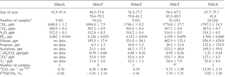
Table 2. Mixing Ratios (Mean and 1 Variation) for the Five Types of Air Masses Encountered by the R/V Ronald Brown During INDOEX SHmX SHmT NHmT NHcT NHcX Day of year 43.5–47.4 48.3–57.6 76.2–77.7 58.1–67.2 67.7–75.7 78.6–79.2 79.8–81.2 85.5–89.5 81.8 Number of samplesa 9 (0) 18 (2) 9 (8) 33 (25) 24 (24) CH4, ppb 1688.8⫾ 1.2 1694.8⫾ 7.5 1746.1⫾ 8.2 1774.0⫾ 17.7 1787.3⫾ 14.5 CO2, ppm 360.9⫾ 0.3 361.2⫾ 0.9 365.8⫾ 0.4 367.1⫾ 0.8 367.4⫾ 0.7 N2O, ppb 312.5⫾ 0.1 312.8⫾ 0.3 314.2⫾ 0.4 314.4⫾ 0.5 314.3⫾ 0.5 SF6, ppt 4.082⫾ 0.018 4.126⫾ 0.033 4.312⫾ 0.034 4.329⫾ 0.059 4.384⫾ 0.040 Ethane, ppt no data 193.5⫾ 17.9 331.8⫾ 30.1 402.9⫾ 125.1 926.9⫾ 429.0 Propane, ppt no data 6.5⫾ 1.2 10.0⫾ 1.3 20.2⫾ 11.0 132.5⫾ 133.9 Acetylene, ppt no data 21.1⫾ 4.6 44.2⫾ 17.3 133.2⫾ 48.8 169.3⫾ 59.8 C2H2/CO, ppt/ppb no data 0.39⫾ 0.06 0.48⫾ 0.16 0.89⫾ 0.26 1.31⫾ 0.43 CO,bppb no data 55.8⫾ 9.0 92.8⫾ 6.9 154.7⫾ 30.8 127.1⫾ 9.2 O3,cppb no data 11.8⫾ 2.6 12.5⫾ 1.3 24.4⫾ 7.9 35.8⫾ 8.6 Number of samples 1 3 1 7d 3 14CO, cm⫺3airSTP 8.70 6.20⫾ 0.40 8.19 9.72⫾ 1.30 13.59⫾ 3.15 ␦18O(CO), ‰ ⫺6.56 ⫺5.41 ⫾ 1.14 ⫺1.41 1.76⫾ 1.31 3.02⫾ 1.50
aNumber of NMHC measurements (only made for legs 2 and 3) are given in parentheses. bCO with courtesy of J. Johnson (continuous measurements [Stehr et al., 2002].
cO
3with courtesy of J. Stehr (continuous measurements [Stehr et al., 2002]). dCarbon monoxide 14 sample 16 was lost during accelerator mass spectrometry.
tance to the coast lengthens (⬃DOY 70–75.7). The isolated acetylene and CO peaks (DOY 73–75) were probably related to input from combustion processes [Wisthaler et al., 2002], supported by the trajectories which were tangent to the coast-line. Compared to the relative uniform trace gas composition in the maritime regimes and the characteristic air mass origin of the NHcX regime, the NHcT air mass type composed of several quite different air parcels and a more detailed distinc-tion is made (Table 3).
[31] During the NHcT “Calcutta” event (DOY 64.2-65.2)
the air parcels that crossed the ship track had passed the highly populated area of Calcutta (trajectory a, via F3), and thus were
influenced by combustion processes, manifested by high levels of CO,18O(CO), C2H2, CO2, and CH4(Figure 2). During the
NHcT “west coast” event (DOY 65.7-67.2), weaker pollution was seen as the air parcels reached the sampling site via the west coast of India (trajectory b). Ethane and propane were comparable during both periods.
4.1.2. Leg 3
[32] The trajectory-based air mass classification attributed
all air masses probed during leg 3 (occurred in the Bay of Bengal) to NHmT air since the trajectories stayed over the ocean for at least 5 days before encounter. The trace gas data, however, revealed a quite high degree of pollution, CO varied between 100 and 170 ppb, and acetylene varied between 60 ppt and 150 ppt. Meteorological analyses indicated synoptical dis-turbances with small-scale local winds and thus less reliable back trajectories for this time. The trace gas data suggest that the air masses were imported from southeast Asia via channels
F3(and F4) before examination. Conclusively, all air masses
during leg 3 were assigned to NHcT air (although the back trajectories suggest NHmT air).
[33] For NHcT, “high NMHC” event (DOY 87.3–88.1),
compared to NHmT air, acetylene and ethane were strongly elevated concurrent with slightly enhanced levels of CO and O3 (Tables 2 and 3), which most likely points to an aged
biomass burning plume [Mauzerall et al., 1998; Singh et al.,
2000]. A thunderstorm on early DOY 87 may have mixed several air masses, making back trajectory analysis unreliable (trajectory f).
[34] For NHcT, “low NMHC” event (DOY 88.5–88.6), a
short, but sharp minimum in NMHC, O3(Figure 2a), and SF6
(not shown) points to a maritime origin of this air mass, in contrast to the modestly enhanced levels of CO, CO2, and
CH4. As only two samples are available and the trajectories
changed during this time period the origin of these air masses could not be determined (trajectories g and h).
[35] For NHcT, “Bay of Bengal” event (DOY 88.9–89.3),
tracers for combustion processes such as CO,␦18O(CO), C 2H2,
CO2, and CH4 were high (Table 3), in companion with
en-hanced levels of other NMHCs and O3. This again points to
continental air masses imported into the Bay of Bengal by airflow F3.
[36] In summary, the five air mass types NHcT, NHcX,
NHmT, SHmT, and SHmX crossed by the Ronald Brown show very different mean mixing ratios of the measured compounds (Table 2). The differences between these mean values are often higher than the variance within each type of air mass which confirms the suitable identification of the individual air masses. The mixing ratios of most longer-lived compounds (CH4, CO2, N2O, SF6, ethane, propane, acetylene) and the
ratio C2H2/CO maximized in NHcX air, followed by NHcT,
NHmT, SHmT, and SHmX air. For CH4, CO2, N2O, and SF6,
the longest-lived and thus the most well-mixed trace gases examined, the interhemispheric gradient is much larger than the differences between the individual types of air masses within one hemisphere. The most pronounced pollution event (DOY 67.7–75.7, in sum 8 days) was attributed to long-range transport from the extratropics, which will be analyzed in more detail now.
4.2. Influence of Meridional Long-Range Transport on the Observed Trace Gas Variability
[37] The strongly declining OH concentrations in winter
toward high northern latitudes lead to a well-known accumu-Table 3. Mixing Ratios (Mean and 1 Variation) for Air Masses Classified as NHcT
Specific Event
Leg 2 Leg 3
Calcutta West CoastIndia High NMHC Low NMHC BengalBay of
Day of year 64.2–65.2 65.7–67.2 87.3–88.1 88.5–88.6 88.9–89.3 Number of samplesa 4 (4) 4 (3) 4 (4) 2 (2) 4 (4) CH4, ppb 1804.0⫾ 1.0 1781.2⫾ 11.3 1755.7⫾ 5.6 1765.7⫾ 2.8 1772.5⫾ 0.5 CO2, ppm 368.1⫾ 0.5 367.0⫾ 0.8 366.5⫾ 0.4 367.3⫾ 0.1 367.5⫾ 0.2 N2O, ppb 315.4⫾ 0.3 315.1⫾ 0.4 314.0⫾ 0.3 314.0⫾ 0.0 314.4⫾ 0.1 SF6, ppt 4.412⫾ 0.019 4.359⫾ 0.053 4.333⫾ 0.062 4.275⫾ 0.065 4.305⫾ 0.062 Ethane, ppt 565.6⫾ 32.2 544.2⫾ 86.6 450.3⫾ 43.7 195.4⫾ 24.6 370.3⫾ 9.8 Propane, ppt 29.7⫾ 4.3 36.9⫾ 18.9 21.2⫾ 2.1 6.3⫾ 0.1 17.1⫾ 0.9 Acetylene, ppt 225.7⫾ 7.1 141.8⫾ 21.9 134.0⫾ 9.4 66.6⫾ 13.7 138.5⫾ 9.0 C2H2/CO, ppt/ppb 1.13⫾ 0.07 0.98⫾ 0.09 1.23⫾ 0.20 0.44⫾ 0.08 0.86⫾ 0.14 CO,bppb 203.1⫾ 4.8 146.1⫾ 18.9 119.0⫾ 9.8 151.2⫾ 2.6 162.9⫾ 3.0 O3,cppb 30.1⫾ 3.4 35.9⫾ 3.0 24.7⫾ 0.5 12.2⫾ 0.9 22.4⫾ 1.5 Number of samples 1 1 1 - 1 (0)d 14CO, cm⫺3airSTP 11.68 10.14 9.00 - -␦18O(CO), ‰ 3.45 1.78 0.93 - 2.26
aNumber of NMHC measurements are given in parentheses.
bCO with courtesy of J. Johnson (continuous measurements [Stehr et al., 2002]). cO
3with courtesy of J. Stehr (continuous measurements [Stehr et al., 2002]). dCarbon monoxide 14 sample 16 was lost during accelerator mass spectrometry.
lation of various medium- and long-lived trace gases, the “NH winter plume” (hydrocarbons, CO, etc.) [Penkett and Brice, 1986; Novelli et al., 1998; Bonsang and Boissard, 1999]. Strong inner NH gradients are formed for many NMHC [Ehhalt et al., 1985; Rudolph, 1988; Boissard et al., 1996], CH4, and CO [e.g.,
Novelli et al., 1995, 1998], which peak in late winter/early spring
[Blake and Rowland, 1986; Rudolph, 1995].
[38] It is analyzed now if these strong latitudinal gradients
are, at least partially, responsible for the observed trace gas variability. Carbon monoxide 14 is an ideal tracer for the lat-itudinal origin of an air mass, as the nature of its main source and its sink lead to a clear latitudinal gradient in14CO [Jo¨ckel
et al., 1999] with weak longitudinal variations. Carbon
monox-ide 14 is mainly produced by a well-defined diffuse source (cosmic radiation), its production rate varies only with latitude with a minimum in the tropics (changes in solar activity and solar proton events can be disregarded). The main sink of
14CO, the OH radical shows a meridional gradient with a
maximum in the tropics. Typical NH background values for February-March are about 20 molecules cm⫺3in the
midlati-tudes (47⬚N) [Gros et al., 2001] and about 9 molecules cm⫺3in
the tropics (13⬚N) [Mak and Southon, 1998].
[39] During INDOEX the NH14CO concentrations (⬃8 to
17 molecules cm⫺3, Figure 2b) are comparable to these values,
although the latitudinal range is much smaller (⬃3 to 18⬚N), which already indicates that the observed large14CO variation
is related to the different latitudinal origins. This relationship is clearly illustrated in Figure 4 (except for samples 13–15 discussed later). Carbon monoxide 14 shows a compact corre-lation (r2ⱖ 0.99) with the latitudinal origin of the 5-day back
trajectories in both hemispheres. Five-day back trajectories were used, being a compromise between the declining reliabil-ity of back trajectories with time [Stohl, 1998] and the typical
transport timescale of Rossby waves that are mostly responsi-ble for the advection of extratropical air masses to the Indian Ocean. Moreover, an excellent agreement is found for the gradients and the values with the estimated latitudinal 14CO
gradient [Jo¨ckel, 2000]. The foregoing reveals that the 14CO
variability observed during INDOEX is almost exclusively caused by long-range transport, and that the available back trajectories are reliable. Furthermore, the high14CO value of
sample 7 impressively supports the extratropical origin of the air masses encountered around DOY 69.
[40] The14CO excess detected in samples 13 to 15 (leg 3)
shows the impact of (14C containing) biogenic CO (Figure 4),
which is most probably related to biomass burning. This claim is supported by the relatively high ␦18O(CO) values of those
three samples (Figure 2b), as well as the enhanced C2H2
mix-ing ratios. Since 10 ppb CO of biogenic origin adds 0.3814CO
molecules cm⫺3 (STP air) [Brenninkmeijer, 1993], the 14CO
excess of sample 15 would be equivalent to 85 ppb additional biogenic CO. This roughly agrees with the observed CO excess of sample 15 of⬃60 ppb when assuming the observed NHmT CO mixing ratio of (92.8⫾ 6.9) ppb (Table 2) as background. [41] The successful use of the back trajectories for14CO is
now applied on hydrocarbons. For this the mixing ratios of propane, ethane, and CH4are displayed versus the latitudinal
origin of the 5-day back trajectories (Figure 5). Two regimes become visible. First, low mixing ratios and no significant cor-relation with latitude south of⬃16⬚N, in particular obvious for propane that is ⬍25 ppt south of ⬃16⬚N, representing back-ground conditions. Second, progressively increasing mixing ra-tios with latitude north of⬃16⬚N. This confirms that the ob-served trace gas variability primarily reflects the latitudinally varying origin of the sampled air masses and that 16⬚N is about the border between regions recently influenced by continental outflow and more pristine areas.
[42] Moreover, it demonstrates that long-range advection
from the extratropical NH strongly contributes to the pollution of the Indian Ocean (at least during INDOEX) and that a significant fraction of the “NH winter plume” is decomposed at lower latitudes, in agreement with model results [Gupta et al., 1998]. Nevertheless, this finding does not imply that the extra-tropical NH is the major source of pollution to the Indian Ocean (via F2). Severe pollution from local sources, especially
from the Calcutta region, was intersected near the tip of India while F3 was active (DOY 58–59, 64–65) and (as already
noted) F3 and F4 are usually more persistent. Additionally,
these recent air masses are expected to be rich in NOx(in
contrast to aged NHcX air) which is required to generate O3.
[43] Worth mentioning is that the latitudinal CH4gradient
of (1.7⫾ 0.2) ppb / ⬚N (r2⫽ 0.66, except samples south of the
chemical ITCZ, Figure 5) agrees reasonably with⬃2.2 ppb/ ⬚N and⬃1.9 ppb / ⬚N extracted from several latitudinal distribu-tions (annual means, 1984–1993) [Dlugokencky et al., 1994] and retrieved from NOAA/CMDL data for March, 1999.
4.3. Discussion of the Use of the C2H2/CO Ratio
As a Measure for Atmospheric Processing
[44] Acetylene and CO have comparable atmospheric
cy-cles. Both are largely combustion products and are removed by the reaction with OH. Owing to the difference in lifetime against OH (for C2H2 ⬃1/3 of that of CO, Table 1)
photo-chemical aging of an air mass after its emissions leads to decreasing C2H2/CO ratios. A competing process also leading
to a decrease of the C2H2/CO ratio is mixing. Thus C2H2/CO
Figure 4. Concentration of14CO versus latitudinal origin of
5-day back trajectory. Linear fits for SH and NH (13,14,15 excluded) shown as dashed and solid lines, respectively. Me-ridional average according to a 14CO climatology (based on
more than 1000 measurements from 15 stations and 156 cam-paigns) [Jo¨ckel, 2000] is shown as doted line. These data are standardized to the global average14CO production rate from
1955 to 1988 which approximately matches the production rate for 1999.
contains information on the sum of mixing and photochemistry (“atmospheric processing”) [McKeen and Liu, 1993]. Note that local sources or mixing with different air masses corrupt the C2H2/CO ratio.
[45] On the basis of this tool, Smyth et al. [1996, 1999]
concluded that “mixing” strongly dominated over “chemistry” during the Pacific Exploratory Missions (PEM) in the free atmosphere. Rapidly decreasing C2H2/CO ratios with a
half-lifetime of typically 1–3 days were recorded, which primarily reflected the speed of mixing with background air.
[46] It is demonstrated now that the information derived
from the C2H2/CO ratio differs strongly from the results by
Smyth et al. [1996, 1999] when applied to the measurements
over the Indian Ocean. As seen in Figure 2, maximum C2H2/CO ratios of up to 2.3 ppt/ppb were encountered in air
masses that originated from the extratropical free troposphere (around DOY 69) and subsided to the marine boundary layer near the coastline. According to Smyth et al. [1999] such C2H2/CO ratios should mark air mass ages of⬍2 days, which
seems to be unrealistic as the back trajectories show that the “source area” is more than 5 days away. The following condi-tions encountered during INDOEX and the PEM missions are different.
1. In the extratropical NH winter/early spring, C2H2
strongly accumulates (see section 4.2), so that the C2H2/CO
background ratio is much higher than in the free troposphere over the Pacific (⬍0.5 ppt/ppb). Therefore mixing with back-ground air has a smaller impact on the decline of the C2H2/CO
ratio compared to the free troposphere over the Pacific. This claim is supported by observations by Roths and Harris [1996] and Boissard et al. [1996], who found 100–130 ppb CO and 300–400 ppt C2H2, respectively, in the free troposphere at
30⬚– 45⬚N in January (Tropospheric Ozone Experiment (TROPOZ) II), which corresponds to a C2H2/CO ratio of⬃3
ppt/ppb. These contrasting conditions are reflected in the IN-DOEX data (Figure 6). Indeed, the air masses with the highest C2H2/CO ratios originate from the extratropics (see NHcX,
Table 2, Figure 2a) where the C2H2/CO background ratio is
much higher than in the tropics.
2. Mixing with background air is reduced in the planetary boundary layer compared to the free troposphere, which slows down the decrease of the C2H2/CO ratio with time. Note that
Smyth et al. [1996, 1999] have omitted the measurements made
in the boundary layer from their analysis.
[47] Conclusively, the C2H2/CO ratio during INDOEX was
less affected by mixing compared to the free troposphere over the Pacific (i.e., during the PEM missions), where mixing was found to be the dominant effect influencing the C2H2/CO
ratio. Therefore the relationship between the C2H2/CO ratio
and air mass age given by Smyth et al. [1996, 1999] which is Figure 5. Mixing ratios of (a) propane, (b) ethane, and (c)
methane versus latitudinal origin of 5-day back trajectory, di-vided up in north of⬃16⬚N and south of ⬃16⬚N (see section 4.2). Days of year (DOY) are noted.
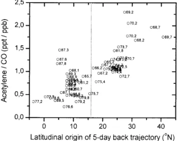
Figure 6. Ratio of acetylene to carbon monoxide (ppt/ppb) versus latitudinal origin of 5-day back trajectory, divided up in north of⬃16⬚N and south of ⬃16⬚N. Days of year (DOY) are noted.
based on the dominance of mixing is not applicable during INDOEX for air masses advected from latitudes north of ⬃16⬚N.
[48] Note that in areas which were not recently affected by extratropical air masses (south of⬃16⬚N), enhanced C2H2/CO
ratios of up to 1.5 (on DOY 87), the “high NMHC” event (Table 3, Figure 2a), were related to an aged biomass burning plume (section 4.1.2, second paragraph). However, compared to PEM-West B, the C2H2/CO ratios were much lower (Table
4), which demonstrates that the air masses intersected by the R/V Ronald Brown were less affected by fresh emissions from combustion processes, which is supported by other trace gas data (see section 5).
5. Comparison With Previous Observations
[49] Compared to the pre-INDOEX ship study by Rhoads et al. [1997] (March-April 1995), more severe pollution wasencountered during INDOEX in NH air masses, supported, among others, by the higher mixing ratios of CO and O3[Stehr
et al., 2002]. Tracers for combustion (see Table 1) peaked in
the Arabian Sea (in agreement with Lal et al. [1998] and Naja
et al. [1999]) and the Bay of Bengal, both areas not visited by Rhoads et al. [1997]. These regions are surrounded by densely
populated areas and are affected by advection from the extra-tropics. Rhoads et al. [1997] found two SH maritime regimes, based on a rise of CO and non-sea salt aerosol (but without a corresponding change in the back trajectories). The INDOEX trace gas data and the back trajectory calculations support the presence of two SH air mass types (SHmT and SHmX), see Table 2. The INDOEX data confirm the distinction in mete-orological regimes made by Rhoads et al. [1997] and W. P. Ball et al. (unpublished manuscript, 2002) and give further evidence for the importance of transport of anthropogenic emissions to the remote Indian Ocean.
[50] Ethane and acetylene mixing ratios in the NHcX
re-gime are comparable to previous marine springtime measure-ments in the tropics/subtropics [Rudolph and Ehhalt, 1981;
Rudolph and Johnen, 1990; Atlas et al., 1993; Donahue and Prinn, 1993] and in the free troposphere at 30⬚–40⬚N (1–2 ppb and 0.2–0.5 ppb, respectively) [Boissard et al., 1996], which supports the importance of advection from the extratropical NH. Bonsang et al. [1988] reported similar ethane values in coastal vicinity of Africa, but acetylene remained much lower (⬍30 ppt). Propane values are similar to several reports
[Ru-dolph and Ehhalt, 1981; Bonsang et al., 1988; Ru[Ru-dolph and Johnen, 1990; Atlas et al., 1993; Donahue and Prinn, 1993].
[51] Numerous NHcT and most NHmT propane measure-ments are at the lower end of previous reports, which empha-sizes the remote character already seen at the back trajectories. Only Rudolph and Johnen [1990] and Atlas et al. [1993] re-ported comparable low propane mixing ratios.
[52] The mixing ratios of ethane and acetylene in SHmT air
are in the range of previous observations in the southern In-dian Ocean [Kanakidou et al., 1988; Bonsang et al., 1990;
Touaty et al., 1996] and other tropical Ocean sites [Blake and Rowland, 1986; Rudolph and Johnen, 1990] in late winter/early
spring. Rudolph [1995] retrieved⬃270–300 ppt ethane from a database for February with a gradual transition from NH to SH. As pointed out by Rudolph [1995], this difference to the stepwise change observed by Donahue and Prinn [1993] (as well as during INDOEX, Figure 2a, DOY 79), is the result of averaging. Due to the variable location of the chemical ITCZ (south or north of the equator), the sharp drop is smoothed out in the longitudinally averaged latitudinal profile given by
Ru-dolph [1995]. Saito et al. [2000] reported 3–6 times higher
acetylene values in the Indian Ocean, probably due to the encounter of strong pollution. Comparable propane levels were observed in the remote Atlantic ocean [Rudolph and
Johnen, 1990].
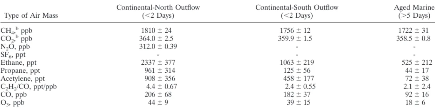
[53] During PEM-West B (February-March, 1994) where
the Asian outflow to the Pacific Ocean was analyzed, distinctly higher concentrations of pollutants were encountered below 2 km altitude [Blake et al., 1997; Talbot et al., 1997]. All trace gases except CO2were significantly higher (Table 4) in
conti-nentally influenced air masses (origin⬎20⬚N, classified by
Tal-bot et al. [1997] as continental north). Compared to the fresh
continental outflow encountered during PEM below 5 km al-titude, the air masses sampled by the Ronald Brown were aged, i.e., had no contact with landmasses for more than 4 days. Even less polluted air masses classified by Talbot et al. [1997] as continental south (origin⬍20⬚N) showed higher levels of typ-ical pollution tracers, e.g., CO and acetylene. Aged marine masses [Talbot et al., 1997] and NHmT air during INDOEX had a more comparable trace gas composition (Table 4) (ex-cept for propane), but the slightly higher acetylene and ethane mixing ratios document a less pristine character even for the aged maritime air.
Table 4. Mixing Ratios (Mean and 1 Variation) at Altitudes ⬍2 km During PEM-West B (February-March 1994)a
Type of Air Mass Continental-North Outflow(⬍2 Days) Continental-South Outflow(⬍2 Days) Aged Marine(⬎5 Days)
CH4,bppb 1810⫾ 24 1756⫾ 12 1722⫾ 31 CO2,bppb 364.0⫾ 2.5 359.9⫾ 1.5 358.5⫾ 0.8 N2O, ppb 312.0⫾ 0.39 - -SF6, ppt - - -Ethane, ppt 2337⫾ 377 1063⫾ 219 525⫾ 212 Propane, ppt 961⫾ 314 125⫾ 56 44⫾ 17 Acetylene, ppt 908⫾ 356 458⫾ 177 72⫾ 38 C2H2/CO, ppt/ppb 4.4⫾ 0.67 2.4⫾ 0.55 2.1⫾ 2.4 CO, ppb 206⫾ 68 182⫾ 37 92⫾ 16 O3, ppb 44⫾ 9 39⫾ 15 18⫾ 6
aFrom Talbot et al. [1997]. bCO
6. Conclusions
[54] During the INDOEX R/V Ronald Brown cruise in the
Indian Ocean (February-March 1999, track in Figure 1), pro-nounced variability in various medium- and long-lived trace gases, such as NMHC, CH4, CO, and CO2, was observed. This
variability was partially related to nearby continental outflow from India and Southeast Asia via the airflows F3and F4(the
four prevailing airflows are shown in Figure 1), but the stron-gest pollution event was caused by long-range transport from the extratropical NH (Middle East and probably even Europe) via airflow F2. In comparison to the PEM-West B expedition
over the Pacific Ocean (February-March 1994), little fresh pollution was encountered by the R/V Ronald Brown; most air masses had no contact with landmasses for more than 4 days. Because of the atypical meteorological situation during IN-DOEX [Verver et al., 2001], it can be expected that the conti-nental outflow from India and Southeast Asia via F3and F4is
usually more persistent in the lower troposphere. Note that throughout the INDOEX campaign layers of fresh pollution were actually encountered, but mainly above the marine boundary layer (MBL), demonstrated by extensive airborne trace gas and aerosol measurements [Mayol-Bracero et al., 2002, Sheridan et al., 2002].
[55] The presence of long-range advection of pollutants in
the Indian Ocean was excellently confirmed by the measured
14CO. Using 5-day back trajectories, a compact latitudinal
gra-dient (r2ⱖ 0.99) of (0.29 ⫾ 0.01) molecules cm⫺3/⬚N in the NH
and (0.077⫾ 0.004) molecules cm⫺3/⬚S in the SH was inferred,
in excellent agreement with the 14CO climatology by Jo¨ckel
[2000].
[56] For air masses that were imported from latitudes north
of⬃16⬚N, the C2H2/CO ratio was found to be unsuitable as a
measure for atmospheric processing as defined by Smyth et al., [1996, 1999] for the PEM missions. This difference is caused by the lower impact of mixing during INDOEX compared to PEM, where mixing was found to be the dominant effect in-fluencing the C2H2/CO ratio. First, due to the strong
accumu-lation of pollutants in the winter northern hemisphere and the corresponding elevated background C2H2/CO ratio of typically
3 ppt/ppb (much higher than the⬃0.5 ppt/ppb during PEM-West B), the impact of mixing on the C2H2/CO ratio is
re-duced. Second, mixing with background air in the marine boundary layer is small compared to the free troposphere. Therefore elevated C2H2/CO ratios during INDOEX mostly
reflected import of air masses from the extratropics. However, south of⬃16⬚N enhanced C2H2/CO ratios, as observed in the
Bay of Bengal, could be assigned to biomass burning, sup-ported by other NMHC as well as the 14C/12C and18O/16O
isotope ratios of CO.
[57] Acknowledgments. The work was supported by the BMBF under the grant 01LA9831/2. We thank J. E. Johnson and J. W. Stehr for provision of the CO and O3data, and the National Oceanic and Atmospheric Administration (NOAA) Climate Monitoring and Diag-nostics Laboratory (CMDL) Carbon Cycle Group for reference data on CH4, CO, and CO2. We are grateful to R. Hofmann, W. Hanewacker, C. Koeppel, and R. Schmunck for their careful analyses. We especially thank the two anonymous reviewers for their valuable comments on the manuscript.
References
Apel, E. C., and J. G. Calvert, Initial results from the nonmethane hydrocarbon intercomparison experiment, J. Chin. Chem. Soc., 41, 279–286, 1994.
Apel, E. C., J. G. Calvert, and F. C. Fehsenfeld, The nonmethane hydrocarbon intercomparison experiment (NOMHICE): Tasks 1 and 2, J. Geophys. Res., 99, 16,651–16,664, 1994.
Apel, E. C., J. G. Calvert, T. M. Gilpin, F. C. Fehsenfeld, D. D. Parrish, and W. A. Lonneman, The nonmethane hydrocarbon intercompari-son experiment (NOMHICE): Task 3, J. Geophys. Res., 104, 26,069– 26,086, 1999.
Arlander, D. W., D. R. Cronn, J. C. Farmer, F. A. Menzia, and H. H. Westberg, Gaseous oxygenated hydrocarbons in the remote marine troposphere, J. Geophys. Res., 95, 16,391–16,403, 1990.
Atlas, E., W. Pollock, J. Greenberg, L. Heidt, and A. M. Thompson, Alkyl nitrates, nonmethane hydrocarbons, and halocarbon gases over the equatorial Pacific Ocean during SAGA 3, J. Geophys. Res.,
98, 16,933–16,947, 1993.
Baldy, S., G. Ancellet, M. Bessafi, A. Badr, and D. L. S. Luk, Field observations of the vertical distribution of tropospheric ozone at the Island of Reunion (southern tropics), J. Geophys. Res., 101, 23,835– 23,849, 1996.
Bange, H. W., S. Rapsomanikis, and M. O. Andreae, Nitrous oxide emissions from the Arabian Sea, Geophys. Res. Lett., 23, 3175–3178, 1996.
Bange, H. W., R. Ramesh, S. Rapsomanikis, and M. O. Andreae, Methane in surface waters of the Arabian Sea, Geophys. Res. Lett.,
25, 3547–3550, 1998.
Blake, D. R., and F. S. Rowland, Global atmospheric concentrations and source strength of ethane, Nature, 321, 231–233, 1986. Blake, N. J., D. R. Blake, T. Y. Chen, J. E. Collins, G. W. Sachse, B. E.
Anderson, and F. S. Rowland, Distribution and seasonality of se-lected hydrocarbons and halocarbons over the western Pacific basin during PEM-West A and PEM-West B, J. Geophys. Res., 102, 28,315–28,331, 1997.
Boissard, C., B. Bonsang, M. Kanakidou, and G. Lambert, Tropoz II -Global distributions and budgets of methane and light hydrocar-bons, J. Atmos. Chem., 25, 115–148, 1996.
Bonsang, B., and C. Boissard, Global distribution of reactive hydro-carbons in the atmosphere, in Reactive Hydrohydro-carbons in the
Atmo-sphere, pp. 209–265, Academic, San Diego, Calif., 1999.
Bonsang, B., M. Kanakidou, G. Lambert, and P. Monfray, The marine source of C2-C6aliphatic hydrocarbons, J. Atmos. Chem., 6, 3–20, 1988.
Bonsang, B., M. Kanakidou, and G. Lambert, NMHC in the marine atmosphere: Preliminary results of monitoring at Amsterdam Island,
J. Atmos. Chem., 11, 169–178, 1990.
Bonsang, B., C. Polle, and G. Lambert, Production of non-methane hydrocarbons by seawater, Ann. Inst. O´ ceanogr., 69, 125–128, 1993.
Bra¨unlich, M., Study of the atmospheric carbon monoxide and meth-ane using isotopic analysis, dissertation thesis, Rupertus Carola Univ., Heidelberg, Germany, 2000.
Brenninkmeijer, C. A. M., Measurement of the abundance of14CO in the atmosphere and the13C/12C and18O/16O ratio of atmospheric CO, with application in New-Zealand and Antarctica, J. Geophys.
Res., 98, 10,595–10,614, 1993.
Brenninkmeijer, C. A. M., T. Ro¨ckmann, M. Bra¨unlich, P. Jo¨ckel, and P. Bergamaschi, Review of progress in isotope studies of atmo-spheric carbon monoxide, Chemosphere Global Change Sci., 1, 33– 52, 1999.
Brenninkmeijer, C. A. M., C. Koeppel, T. Ro¨ckmann, D. S. Scharffe, M. Bra¨unlich, and V. Gros, Absolute measurement of the abun-dance of atmospheric carbon monoxide, J. Geophys. Res., 106, 10,003–10,010, 2001.
Butler, J. H., J. W. Elkins, C. M. Brunson, K. B. Egan, T. M. Thomp-son, T. J. Conway, and B. D. Hall, Trace gases in and over the West Pacific and East Indian Oceans during the El Nino-Southern Oscil-lation event of 1987, NOAA Rep. ERL ARL-16, Natl. Oceanic and Atmos. Admin., Boulder, Colo., 1988.
Camel, V., and M. Caude, Trace enrichment methods for the deter-mination of organic pollutants in ambient air, J. Chromatogr. A, 710, 3–19, 1995.
de Laat, A. T. J., M. Zachariasse, G. J. Roelofs, P. van Velthoven, R. R. Dickerson, K. P. Rhoads, S. J. Oltmans, and J. Lelieveld, Tropospheric O3distribution over the Indian Ocean during spring 1995 evaluated with a chemistry-climate model, J. Geophys. Res.,
104, 13,881–13,893, 1999.
DeMore, W. B., S. P. Sander, D. M. Golden, R. F. Hampson, M. J. Kurylo, C. J. Howard, A. R. Ravishankara, C. E. Kolb, and M. J.
Molina, Chemical kinetics and photochemical data for use in strato-spheric modeling, Evaluation 12, JPL Publ., 97-4, 1997.
Dlugokencky, E. J., L. P. Steele, P. M. Lang, and K. A. Masarie, The growth-rate and distribution of atmospheric methane, J. Geophys.
Res., 99, 17,021–17,043, 1994.
Donahue, N. M., and R. G. Prinn, In situ nonmethane hydrocarbon measurements on SAGA 3, J. Geophys. Res., 98, 16,915–16,932, 1993.
Doskey, P. V., The effect of treating air samples with magnesium perchlorate for water removal during analysis for non-methane hy-drocarbons, J. High Resolut. Chromatogr., 14, 724–728, 1991. Doskey, P. V., J. A. Porter, and P. A. Scheff, Source fingerprints for
non-volatile hydrocarbons, J. Air Waste Manage. Assoc., 42, 1437– 1445, 1992.
Draxler, R. R., and G. D. Hess, An overview of the HYSPLIT_4 modelling system for trajectories, dispersion, and deposition, Aust.
Meteorol. Mag., 47, 295–308, 1998.
Ehhalt, D. H., J. Rudoplh, F. X. Meixner, and U. Schmidt, Measure-ments of selected C2-C5 hydrocarbons in the background tropo-sphere: vertical and latitudinal variations, J. Atmos. Chem., 3, 29–52, 1985.
Goyet, C., F. J. Millero, D. W. Osullivan, G. Eischeid, S. J. McCue, and R. G. J. Bellerby, Temporal variations of Pco(2) in surface sea-water of the Arabian Sea in 1995, Deep Sea Res., Part I, 45, 609 – 623, 1998.
Gros, V., N. Poisson, D. Martin, M. Kanakidou, and B. Bonsang, Observations and modeling of the seasonal variation of surface ozone at Amsterdam Island: 1994 –1996, J. Geophys. Res., 103, 28,103–28,109, 1998.
Gros, V., et al., Detailed analysis of the isotopic composition of CO and characterization of air masses arriving at Mount Sonnblick (Austrian Alps), J. Geophys. Res., 106, 3179–3193, 2001.
Gupta, M. L., R. J. Cicerone, D. R. Blake, F. S. Rowland, and I. S. A. Isaksen, Global atmospheric distributions and source strengths of light hydrocarbons and tetrachloroethene, J. Geophys. Res., 103, 28,219–28,235, 1998.
Habram, M., J. Slemr, and T. Welsch, Development of a dual capillary column GC method for the trace determination of C2-C9 hydrocar-bons in ambient air, J. High Resolut. Chromatogr., 21, 209–214, 1998. Helmig, D., Air analysis by gas chromatography, J. Chromatogr. A, 843,
129–146, 1999.
Hough, A. M., Development of a two-dimensional global tropospheric model: Model chemistry, J. Geophys. Res., 96, 7325–7362, 1991. Intergovernmental Panel on Climate Change (IPCC), Climate Change
1994: Radiative Forcing of Climate Change and an Evaluation of the IPCC IS 92 Emissions Scenarios, edited by J. T. Houghton et al., 339
pp., Cambridge Univ. Press, New York, 1995
Jo¨ckel, P., Cosmogenic14CO as tracer for atmospheric chemistry and transport, dissertation thesis, Rupertus Carola Univ., Heidelberg, Germany, 2000.
Jo¨ckel, P., M. G. Lawrence, and C. A. M. Brenninkmeijer, Simulations of cosmogenic14CO using the three-dimensional atmospheric model MATCH: Effects of14C production distribution and the solar cycle,
J. Geophys. Res., 104, 11,733–11,743, 1999.
Johnson, J. E., R. H. Gammon, J. Larsen, T. S. Bates, S. J. Oltmans, and J. C. Farmer, Ozone in the marine boundary layer over the Pacific and Indian Oceans: Latitudinal gradients and diurnal cycles,
J. Geophys. Res., 95, 11,847–11,856, 1990.
Kanakidou, M., B. Bonsang, J. C. Le Roulley, G. Lambert, D. Martin, and G. Sennequier, Marine source of atmospheric acetylene, Nature,
333, 51–52, 1988.
Kurdziel, M., The effect of different drying agents on the analytical data for non-methane hydrocarbon concentrations in ambient air samples, Chem. Anal. (Warsaw), 43, 387–397, 1998.
Lal, S., M. Naja, and A. Jayaraman, Ozone in the marine boundary layer over the tropical Indian Ocean, J. Geophys. Res., 103, 18,907– 18,917, 1998.
Lewis, A. C., J. B. McQuaid, N. Carslaw, and M. J. Pilling, Diurnal cycles of short-lived tropospheric alkenes at a north Atlantic coastal site, Atmos. Environ., 33, 2417–2422, 1999.
Maiss, M., L. P. Steele, R. J. Francey, P. J. Fraser, R. L. Langenfelds, N. B. A. Trivett, and I. Levin, Sulfur hexafluoride - A powerful new atmospheric tracer, Atmos. Environ., 30, 1621–1629, 1996. Mak, J. E., and C. A. M. Brenninkmeijer, Compressed air sample
technology for isotopic analysis of atmospheric carbon monoxide, J.
Atmos. Oceanic Technol., 11, 425–431, 1994.
Mak, J. E., and J. R. Southon, Assessment of tropical OH seasonality using atmospheric 14CO measurements from Barbados, Geophys.
Res. Lett., 25, 2801–2804, 1998.
Matusˇka, P., M. Koval, and W. Seiler, A high resolution GC-analysis method for determination of C2-C10hydrocarbons in air samples, J.
High Resolut. Chromatogr. Chromatogr. Commun., 9, 577–583, 1986.
Mauzerall, D. L., J. A. Logan, D. J. Jacob, B. E. Anderson, D. R. Blake, J. D. Bradshaw, B. Heikes, G. W. Sachse, H. Singh, and B. Talbot, Photochemistry in biomass burning plumes and implications for tropospheric ozone over the tropical South Atlantic, J. Geophys.
Res., 103, 8401–8423, 1998.
Mayol-Bracero, O. L., T. W. Kirchstetter, T. Novakov, M. O. Andreae, R. Gabriel, and D. G. Streets, Carbonaceous aerosols over the Indian Ocean during INDOEX: Chemical characterization, optical properties, and probable sources, J. Geophys. Res., 107(DX), 10.1029/2000JD000039, in press, 2002.
McKeen, S. A., and S. C. Liu, Hydrocarbon ratios and photochemical history of air masses, Geophys. Res. Lett., 20, 2363–2366, 1993. Mitra, A. P., INDOEX (India): Introductory note, Curr. Sci., 76, 886–
889, 1999.
Mitra, S., and C. Yun, Continuous gas chromatographic monitoring of low concentration sample streams using an on-line microtrap,
J. Chromatogr., 648, 415–421, 1993.
Naja, M., S. Lal, S. Venkataramani, K. S. Modh, and D. Chand, Variabilities in O3, NO, CO and CH4over the Indian Ocean during winter, Curr. Sci., 76, 931–937, 1999.
Novelli, P. C., T. J. Conway, E. J. Dlugokency, and P. P. Tans, Recent changes in atmospheric carbon dioxide, methane and carbon mon-oxide, and the implications of these changes on global climate, WMO
Bull., 44, 32–37, 1995.
Novelli, P. C., K. A. Masarie, and P. M. Lang, Distributions and recent changes of carbon monoxide in the lower troposphere, J. Geophys.
Res., 103, 19,015–19,033, 1998.
Penkett, S. A., and K. A. Brice, The spring maximum in photo-oxidants in the Northern Hemisphere troposphere, Nature, 319, 655–657, 1986.
Plass-Du¨lmer, C., R. Koppmann, M. Ratte, and J. Rudolph, Light nonmethane hydrocarbons in seawater, Global Biogeochem. Cycles,
9, 79–100, 1995.
Rasmussen, R. A., C. W. Lewis, R. K. Stevens, W. D. Ellenson, and S. L. Dattner, Removing CO2from atmospheric samples for radio-carbon measurements of volatile compounds, Environ. Sci. Technol.,
30, 1092–1097, 1996.
Rhoads, K. P., P. Kelley, R. R. Dickerson, T. P. Carsey, M. Farmer, D. L. Savoie, and J. M. Prospero, Composition of the troposphere over the Indian Ocean during the monsoonal transition, J. Geophys.
Res., 102, 18,981–18,996, 1997.
Roths, J., and G. W. Harris, The tropospheric distribution of carbon monoxide as observed during the TROPOZ II experiment, J. Atmos.
Chem., 24, 157–188, 1996.
Rudolph, J., Two-dimensional distribution of light hydrocarbons: Re-sults from the STRATOZ III experiment, J. Geophys. Res., 93, 8367– 8377, 1988.
Rudolph, J., The tropospheric distribution and budget of ethane, J.
Geophys. Res., 100, 11,369–11,381, 1995.
Rudolph, J., and D. H. Ehhalt, Measurements of C2-C5hydrocarbons over the North Atlantic, J. Geophys. Res., 86, 11,959–11,964, 1981. Rudolph, J., and F. J. Johnen, Measurements of light atmospheric hydrocarbons over the Atlantic in regions of low biological activity,
J. Geophys. Res., 95, 20,583–20,591, 1990.
Rudolph, J., F. J. Johnen, A. Khedim, and G. Pilwat, The use of automated “on line” gaschromatography for the monitoring of or-ganic trace gases in the atmosphere at low levels, Int. J. Environ.
Anal. Chem., 38, 143–155, 1990.
Rudolph, J., R. Koppmann, and C. Plass-Du¨lmer, The budgets of ethane and tetrachloroethene - Is there evidence for an impact of reactions with chlorine atoms in the troposphere, Atmos. Environ.,
30, 1887–1894, 1996.
Saito, T., Y. Yokouchi, and K. Kawamura, Distributions of C2-C6 hydrocarbons over the western North Pacific and eastern Indian Ocean, Atmos. Environ., 34, 4373–4381, 2000.
Sheridan, P., A. Jefferson, and J. Ogren, Spatial variability of aerosol radiative properties over the Indian Ocean during INDOEX, J.
Geophys. Res., 107(DX), 10.1029/2000JD000166, in press, 2002.
Singh, H. B., and P. B. Zimmerman, Atmospheric distribution and sources of nonmethane hydrocarbons, in Advances in Environmental