HAL Id: hal-01315221
https://hal.inria.fr/hal-01315221
Submitted on 12 May 2016
HAL is a multi-disciplinary open access
archive for the deposit and dissemination of
sci-entific research documents, whether they are
pub-lished or not. The documents may come from
teaching and research institutions in France or
abroad, or from public or private research centers.
L’archive ouverte pluridisciplinaire HAL, est
destinée au dépôt et à la diffusion de documents
scientifiques de niveau recherche, publiés ou non,
émanant des établissements d’enseignement et de
recherche français ou étrangers, des laboratoires
publics ou privés.
Optimal Deployment of Dense WSN for Error Bounded
Air Pollution Mapping
Ahmed Boubrima, Walid Bechkit, Hervé Rivano
To cite this version:
Ahmed Boubrima, Walid Bechkit, Hervé Rivano. Optimal Deployment of Dense WSN for Error
Bounded Air Pollution Mapping. DCOSS 2016 - International Conference on Distributed Computing
in Sensor Systems, May 2016, Washington, DC, United States. �hal-01315221�
Optimal Deployment of Dense WSN for Error
Bounded Air Pollution Mapping
Ahmed Boubrima
∗, Walid Bechkit
∗and Hervé Rivano
∗∗Univ Lyon, Inria, INSA Lyon, CITI, F-69621 Villeurbanne, France
Abstract—Air pollution has become a major issue of mod-ern megalopolis because of industrial emissions and increasing urbanization along with traffic jams and heating/cooling of buildings. Monitoring urban air quality is therefore required by municipalities and by the civil society. Current monitoring systems rely on reference sensing stations that are precise but massive, costly and therefore seldom. In this ongoing work, we focus on an alternative or complementary approach, using a network of low cost and autonomic wireless sensors, allowing for a finer spatiotemporal granularity of air quality sensing. We tackle the optimization problem of sensor deployment and propose an integer programming model, which allows to find the optimal network topology while ensuring air quality monitoring with a high precision and the minimum financial cost. Most of existing deployment models of wireless sensor networks are generic and assume that sensors have a given detection range. This assumption does not fit pollutant concentrations sensing. Our model takes into account interpolation methods to place sensors in such a way that pollution concentration is estimated with a bounded error at locations where no sensor is deployed.
Keywords— Air quality monitoring, Wireless sensor net-works deployment, error bounded mapping.
I. INTRODUCTION
Air pollution affects human health dramatically. According to the World Health Organization (WHO), exposure to air pollution is accountable to seven million casualties in 2012. In 2013, the International Agency for Research on Cancer (IARC) classified particulate matter, the main component of outdoor pollution, as carcinogenic for humans. Air pollution has become a major issue of modern megalopolis, where the majority of world population lives, adding industrial emissions to the consequences of an ever denser urbanization with traffic jams and heating/cooling of buildings. As a consequence, the reduction of pollutant emissions is at the heart of many sustainable development efforts, in particular those of smart cities. Monitoring urban air pollution is therefore required by both municipalities and the civil society.
Current air quality monitoring is mostly operated by in-dependent authorities. Conventional measuring stations are equipped with multiple lab quality sensors. These systems are however massive, inflexible and expensive. An alternative – or complementary – solution would be to use wireless sensor networks (WSN) [1] which consist of a set of lower cost nodes that can measure information from the environment, process and relay them to some base stations, denoted sinks. The progress of electrochemical sensors, that are smaller and cheaper while keeping a reasonable measurement quality, makes the use of WSN for air quality monitoring viable [2].
The main advantage of the use of WSN for air pollution monitoring is to obtain a finer spatiotemporal granularity of measurements, thanks to the resulting lighter installation and operational costs. Although some WSN-based air quality mon-itoring systems are already operating, the deployment issue of these tiny nodes while taking into account the precision of the resulting network has not yet been investigated.
Minimizing the deployment cost is a major challenge in WSN design. The problem consists in determining the optimal positions of sensors and sinks so as to cover the environment and ensure network connectivity while minimizing the deploy-ment cost [3]. The deploydeploy-ment is constrained by the cost of the nodes and sinks, but also by operational costs such as the energy spent by the nodes. The network is said connected if each sensor can communicate information to at least one sink [4]. The coverage issue has often been modeled as a k-coverage problem in which at least k sensors should monitor each point of interest. Most research work on coverage uses a simple detection model which assumes that a sensor is able to cover a point in the environment if the distance between them is less than a radius called the detection range. This can be true for some applications like presence sensors but is not suitable for pollution monitoring. Indeed, a pollution sensor detects pollutants that are brought in contact by the wind. The notion of detection range is thus irrelevant in this context. Therefore, a deployment model is still needed for the air quality monitoring application.
In this ongoing work, we propose an integer programming model (ILP) of WSN deployment for error-bounded air quality mapping. We formulate the constraint of air pollution coverage based on interpolation methods in order to determine the optimal positions of sensors allowing to better estimate pollu-tion concentrapollu-tions at posipollu-tions where no sensor is deployed. We base on the flow problem to formulate the connectivity constraint that ensures that the deployed sensors are able to send pollution data to at least one sink.
II. OPTIMIZATIONMODEL
A. Objective function
We consider as input of our model the map of a given urban area that we call the deployment region. We start by discretizing the deployment region in order to get a set of points P approximating the urban area at a high-scale (|P| = N ). Our goal is to be able to determine with a high precision the concentration value at each point p ∈ P . We ensure that for each point p ∈ P , either a sensor is
deployed or the pollution concentration can be estimated with a high precision based on the data gathered by the neighboring deployed sensors.
In general case, the set P is thus considered as the set of potential positions of WSN nodes. However, in smart cities applications, some restrictions on node positions may apply because of authorization or practical issues. When this is the case, we do not consider as potential positions the points p ∈ P where sensors cannot be deployed. We use decision variables xp resp. yp to specify if a sensor resp. a sink is
deployed at point p or not. Sensors and sinks may have different costs, thus we denote by csensorp resp. csinkp the sensor
resp. the sink deployment cost at position p. The deployment cost function to minimize is thus given as follows:
F =X p∈P csensorp ∗ xp+ X p∈P csinkp ∗ yp (1)
B. Air quality coverage
Using numerical atmospheric dispersion models, we first get simulated pollution concentrations that may be considered as reference pollution concentrations. This does not mean that these reference concentrations are real but they reflect the best today’s pollution knowledge. Let Zp denote the reference
concentration value at point p. Given the set of selected points where sensors will be deployed {p where xp = 1}, we
evaluate the estimated pollution concentrations bZp at points
{p where xp = 0} based on reference values
correspond-ing to the selected points, i.e. based on Zp where p ∈
{p where xp= 1}, as follows: b Zp= P q∈P−{p}Wpq∗ Zq∗ xq P q∈P−{p}Wpq∗ xq , p ∈ P & xp= 0 X q∈P−{p} Wpq∗ xq> 0, p ∈ P & xp= 0 (2)
We ensure that the denominator of bZpis never equal to zero
using the second part of formula 2. The Wpq parameter is the
correlation coefficient between points p and q and is calculated using formula 3 based on the distance between the two points. D(p, q) is the distance function. α is the attenuation coefficient of the correlation distance, this means that for greater values of α, very low correlation coefficients are assigned to far points. The last parameter of formula 3 is the maximum correlation distance, which defines the range of correlated neighboring points of a given point.
In order to take into account the impact of the urban topography on the dispersion of pollutants, let D be the shortest distance along the roads network. This allows to assign small correlation values to points that are separated by buildings, even if they are close.
Wpq= 1 D(p, q)α if q ∈ Disc(p, d) − {p} 0 if q /∈ Disc(p, d) (3)
In order to ensure that the concentration is estimated with high precision at points where no sensor is deployed, we define constraint 4. The Ep parameter corresponds to the estimation
error that is tolerated at point p. The choice of different values of Epin function of p allows to assign low tolerated estimation
errors to locations that are sensitive to air quality such as hospitals, primary schools, etc.
Zbp− Zp ≤ Ep, p ∈ P & xp= 0 (4)
By replacing bZp by its expression given in formula 2, we
obtain the coverage constraints 5 and 6. These two constraints should be linearized in order to get an ILP formulation.
P q∈P−{p}Wpq∗ Zq∗ xq P q∈P−{p}Wpq∗ xq − Zp ≤ Ep, p ∈ P & xp= 0 (5) X q∈P−{p} Wpq∗ xq> 0, p ∈ P & xp= 0 (6)
1) Linearization of constraint 5: The first step is to lin-earize the fraction part; this allows to get constraint 7. We now add xp∗Pq∈P−{p}Wpq∗ |Zq− Zp| to the right member
of constraint 7 to relax it when xp = 1. Hence, we obtain
constraint 8. Finally, we have to linearize the absolute-value function. Hence, we get the linear form of constraint 5 in constraints 9 and 10. X q∈P−{p} Wpq∗ xq∗ (Zq− Zp) ≤ Ep∗ X q∈P−{p} Wpq∗ xq, p ∈ P, xp= 0 (7) X q∈P−{p} Wpq∗ xq∗ (Zq− Zp) ≤ Ep∗ X q∈P−{p} Wpq∗ xq +xp∗ X q∈P−{p} Wpq∗ |Zq− Zp|, p ∈ P (8) X q∈P−{p} Wpq∗ xq∗ (Zq− Zp) ≤ Ep∗ X q∈P−{p} Wpq∗ xq +xp∗ X q∈P−{p} Wpq∗ |Zq− Zp|, p ∈ P (9) X q∈P−{p} −Wpq∗ xq∗ (Zq− Zp) ≤ Ep∗ X q∈P−{p} Wpq∗ xq +xp∗ X q∈P−{p} Wpq∗ |Zq− Zp|, p ∈ P (10)
2) Linearization of constraint 6: The only thing to do to linearize constraint 6 is to relax the constraint when xp = 1.
This can be obtained by replacing the right member of the constraint by −xp, which allows to get the constraint 11.
X
q∈P−{p}
C. Network connectivity
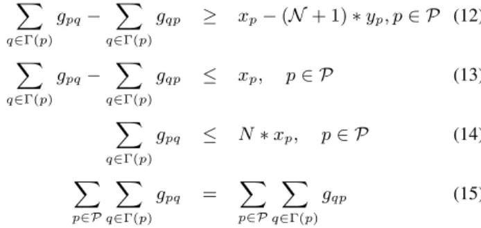
We formulate the connectivity constraint as a network flow problem. We consider the same potential positions set P for sensors and sinks. We first denote by Γ(p), p ∈ P, the set of neighbors of a node deployed at the potential position p, Γ(p) = {q ∈ P where q ∈ Disc(p, R)} where R is the communication range of sensors. Then, we define the decision variables gpq as the flow quantity transmitted from a node
located at potential position p to another node located at potential position q. We suppose that each sensor generates a flow unit in the network, and verify if these units can be recovered by sinks. The following constraints ensure that the deployed sensors and sinks form a connected WSN; i.e. each sensor can communicate with at least one sink.
X q∈Γ(p) gpq− X q∈Γ(p) gqp ≥ xp− (N + 1) ∗ yp, p ∈ P (12) X q∈Γ(p) gpq− X q∈Γ(p) gqp ≤ xp, p ∈ P (13) X q∈Γ(p) gpq ≤ N ∗ xp, p ∈ P (14) X p∈P X q∈Γ(p) gpq = X p∈P X q∈Γ(p) gqp (15)
Constraints 12 and 13 are designed to ensure that each deployed sensor, i.e. such that xp= 1, generates a flow unit in
the network. Constraint 14 ensures that non deployed nodes do not participate in communication. The flow sent by deployed sensors has then to be received by deployed sinks, thanks to constraint 15. At the end, our optimization model can be written as follows:
M inimize (1)
Subject to. (9), (10), (11), (12), (13), (14) and (15)
III. SIMULATION RESULTS
A. Dataset
We perform our simulations on a pollution map generated by an enhanced atmospheric dispersion simulator called SIR-ANE. The dataset has been provided by Air-Rhone-Alpes, which is an observatory for air pollution monitoring within the Lyon region of France. We evaluate our ILP model on the La-Part-Dieu district, which is the heart of the Lyon City. Pol-lution map granularity is around 5 meters and concentrations correspond to the year 2012. We discretize the deployment region which is of around 850mX850m using a resolution of 50 meters, thus we get 306 discrete points. We consider all these points as potential positions of nodes.
B. Results
We study the dependency between the deployment precision and the needed number of sensors under different configura-tions of the correlation distance. Since we are studying the cost of the monitoring precision, we execute only the coverage constraint. We depict in Figure 1 the optimal deployment cost
depending on the tolerated estimation error while consider-ing two different functions of the correlation distance: the euclidean distance and the distance along roads. We notice that the number of sensors decreases as expected with the estima-tion error that is tolerated. Indeed, the interpolaestima-tion method assumes a linear spatial evolution of pollution concentration between points where sensors are deployed (cf eq. (2)). When the tolerated error is small, it is required to deploy sensors at the locations where there is a high variability of pollution concentrations.
Regarding the impact of the distance metric, the distance along roads is obviously larger than the euclidean distance and takes into account the buildings that influence both pollution dispersion and radio propagation. Correlation coefficients (cf eq. (3)) are therefore smaller when using the distance along roads, hence more sensors are required in order to get a better estimation of pollution concentrations.
Fig. 1: Optimal coverage cost vs tolerated estimation error. IV. CONCLUSION
In this ongoing work, we tackled the optimization problem of sensor deployment and proposed an integer programming model computing a cost-optimal network topology while en-suring the mapping of air quality with bounded error. Our idea is to constraint the deployment of sensors by the quality of the pollution estimation that can be interpolated between the sensors. ACKNOWLEDGMENT
This work has been supported by the "LABEX IMU" (ANR-10-LABX-0088) and the "Programme Avenir Lyon Saint-Etienne" of Université de Lyon, within the program "Investissements d’Avenir" (ANR-11-IDEX-0007) operated by the French National Research Agency (ANR).
REFERENCES
[1] A. Kumar, H. Kim, and G. P. Hancke, “Environmental monitoring systems: a review,” Sensors Journal, IEEE, vol. 13, no. 4, pp. 1329–1339, 2013.
[2] M. Mead, O. Popoola, G. Stewart, P. Landshoff, M. Calleja, M. Hayes, J. Baldovi, M. McLeod, T. Hodgson, J. Dicks et al., “The use of electrochemical sensors for monitoring urban air quality in low-cost, high-density networks,” Atmospheric Environment, vol. 70, pp. 186–203, 2013. [3] C. Zhu, C. Zheng, L. Shu, and G. Han, “A survey on coverage and connectivity issues in wireless sensor networks,” Journal of Network and Computer Applications, vol. 35, no. 2, pp. 619–632, 2012.
[4] M. Younis and K. Akkaya, “Strategies and techniques for node placement in wireless sensor networks: A survey,” Ad Hoc Networks, vol. 6, no. 4, pp. 621–655, 2008.