HAL Id: hal-01094444
https://hal-cea.archives-ouvertes.fr/hal-01094444
Submitted on 12 Dec 2014
HAL is a multi-disciplinary open access
archive for the deposit and dissemination of
sci-entific research documents, whether they are
pub-lished or not. The documents may come from
teaching and research institutions in France or
abroad, or from public or private research centers.
L’archive ouverte pluridisciplinaire HAL, est
destinée au dépôt et à la diffusion de documents
scientifiques de niveau recherche, publiés ou non,
émanant des établissements d’enseignement et de
recherche français ou étrangers, des laboratoires
publics ou privés.
Study of HD 169392A observed by CoRoT and HARPS
S. Mathur, H. Bruntt, C. Catala, O. Benomar, G. R. Davies, R. A. García, D.
Salabert, J. Ballot, B. Mosser, C. Régulo, et al.
To cite this version:
S. Mathur, H. Bruntt, C. Catala, O. Benomar, G. R. Davies, et al.. Study of HD 169392A observed
by CoRoT and HARPS. Astronomy and Astrophysics - A&A, EDP Sciences, 2013, 549, pp.A12.
�10.1051/0004-6361/201219678�. �hal-01094444�
DOI:10.1051/0004-6361/201219678
c
ESO 2012
Astrophysics
&
Study of HD 169392A observed by CoRoT and HARPS
?,??,???
S. Mathur
1,2, H. Bruntt
3, C. Catala
4, O. Benomar
5, G. R. Davies
2, R. A. García
2, D. Salabert
6, J. Ballot
7,8, B. Mosser
4,
C. Régulo
9,10, W. J. Chaplin
11, Y. Elsworth
11, R. Handberg
3, S. Hekker
12,11, L. Mantegazza
13, E. Michel
4, E. Poretti
13,
M. Rainer
13, I. W. Roxburgh
14, R. Samadi
4, M. Ste¸´slicki
15,1K. Uytterhoeven
9,10, G. A. Verner
11, M. Auvergne
4,
A. Baglin
4, S. Barceló Forteza
9,10, F. Baudin
16, and T. Roca Cortés
9,101 High Altitude Observatory, NCAR, PO Box 3000, Boulder, CO 80307, USA
e-mail: savita.mathur@gmail.com
2 Laboratoire AIM, CEA/DSM – CNRS – Univ. Paris Diderot – IRFU/SAp, Centre de Saclay, 91191 Gif-sur-Yvette Cedex, France 3 Danish AsteroSeismology Centre, Department of Physics and Astronomy, University of Aarhus, 8000 Aarhus C, Denmark 4 LESIA, UMR 8109, Université Pierre et Marie Curie, Université Denis Diderot, Obs. de Paris, 92195 Meudon Cedex, France 5 Sydney Institute for Astronomy, School of Physics, University of Sydney, NSW 2006, Australia
6 Laboratoire Lagrange, UMR 7293, Universié de Nice Sophia-Antipolis, CNRS, Observatoire de la Côte d’Azur,
06304 Nice Cedex 4, France
7 CNRS, Institut de Recherche en Astrophysique et Planétologie, 14 avenue Édouard Belin, 31400 Toulouse, France 8 Université de Toulouse, UPS-OMP, IRAP, 31400 Toulouse, France
9 Instituto de Astrofísica de Canarias, 38205 La Laguna, Tenerife, Spain 10 Universidad de La Laguna, Dpto de Astrofísica, 38206 Tenerife, Spain
11 School of Physics and Astronomy, University of Birmingham, Edgbaston, Birmingham B15 2TT, UK
12 Astronomical Institute Anton Pannekoek, U. of Amsterdam, PO Box 94249, 1090 GE Amsterdam, The Netherlands 13 INAF – Osservatorio Astronomico di Brera, via E. Bianchi 46, 23807, Merate (LC), Italy
14 Astronomy Unit, Queen Mary University of London, Mile End Road, London E1 4NS, UK 15 Instytut Astronomiczny, Uniwersytet Wroclawski, Kopernika 11, 51-622 Wroclaw, Poland
16 Institut d’Astrophysique Spatiale, UMR 8617, Université Paris XI, Batiment 121, 91405 Orsay Cedex, France
Received 24 May 2012/ Accepted 19 September 2012
ABSTRACT
Context.The results obtained by asteroseismology with data from space missions such as CoRoT and Kepler are providing new insights into stellar evolution. After five years of observations, CoRoT is continuing to provide high-quality data and we here present an analysis of the CoRoT observations of the double star HD 169392, complemented by ground-based spectroscopic observations.
Aims.This work aims at characterising the fundamental parameters of the two stars, their chemical composition, the acoustic-mode global parameters including their individual frequencies, and their dynamics.
Methods.We analysed HARPS observations of the two stars to derive their chemical compositions. Several methods were used and compared to determine the global properties of stars’ acoustic modes and their individual frequencies from the photometric data of CoRoT.
Results.The new spectroscopic observations and archival astrometric values suggest that HD 169392 is a weakly bound wide binary system. We obtained spectroscopic parameters for both components which suggest that they originate from the same interstellar cloud. However, only the signature of oscillation modes of HD 169392 A was measured; the signal-to-noise ratio of the modes in HD 169392B is too low to allow any confident detection. For HD 169392 A we were able to extract parameters of modes for `= 0, 1, 2, and 3. The analysis of splittings and inclination angle gives two possible solutions: one with with splittings and inclination angles of 0.4−1.0 µHz and 20−40◦
, the other with 0.2−0.5 µHz and 55−86◦
. Modelling this star using the Asteroseismic Modeling Portal (AMP) gives a mass of 1.15 ± 0.01 M , a radius of 1.88 ± 0.02 R , and an age of 4.33 ± 0.12 Gyr. The uncertainties come from
estimated errors on the observables but do not include uncertainties on the surface layer correction or the physics of stellar models.
Key words.asteroseismology – methods: data analysis – stars: oscillations – stars: individual: HD 169392
? The CoRoT space mission, launched on December 27 2006, has
been developed and is operated by CNES, with the contribution of Austria, Belgium, Brazil, ESA (RSSD and Science Programme), Germany and Spain.
?? This work is based on ground-based observations made with the
ESO 3.6 m-telescope at La Silla Observatory under the ESO Large Programme LP185-D.0056.
???
Tables5and7are available in electronic form at http://www.aanda.org
1. Introduction
The convective motions in the outer layers of solar-like oscil-lating stars excite acoustic waves that become trapped in the stellar interiors (e.g.,Goldreich & Keeley 1977;Samadi 2011, for a detailed review). The precise frequencies of these pres-sure (p)-driven waves depend on the properties of the medium in which they propagate. Thus, stellar seismology allows us to infer the properties of the Sun and stellar interiors by study-ing and characterisstudy-ing these p modes (e.g.,Gough et al. 1996;
Christensen-Dalsgaard 2002). However, our knowledge of the
A&A 549, A12 (2013)
properties of the stellar interiors depends on our ability to cor-rectly measure the properties of the oscillations modes (e.g.
Appourchaux et al. 1998;Appourchaux 2011).
In recent years the French-led satellite, Convection, Rotation and planetary Transits (CoRoT,Baglin et al. 2006), and NASA’s Keplermission (Koch et al. 2010;Borucki et al. 2010) have pro-vided high-quality, long-term seismic data of solar-like stars. CoRoT has studied some interesting F- and G-type stars (e.g.
Appourchaux et al. 2008;Barban et al. 2009;García et al. 2009;
Deheuvels et al. 2010) including some that host planets (Gaulme et al. 2010;Ballot et al. 2011b;Howell et al. 2012) and others in binary systems (Mathur et al. 2010a). Kepler observations have enabled ensemble asteroseismology of hundreds of solar-like stars (e.g.Chaplin et al. 2011b) as well as precise studies of long time-series with more than eight months of nearly continuous data (Campante et al. 2011;Mathur et al. 2011a;Appourchaux et al. 2012b), and pulsating stars in binary systems (e.g.Hekker et al. 2010b; White et al., in prep.) and in clusters (e.g. Basu et al. 2011;Stello et al. 2011b). The fundamental properties of stars can be inferred by means of asteroseismic quantities either by using scaling relations (e.g.Kjeldsen & Bedding 1995,2011;
Samadi et al. 2007b), or by using stellar models (e.g.Piau et al. 2009;Metcalfe et al. 2010,2012;Creevey et al. 2012;Escobar et al. 2012; Mathur et al. 2012; Mazumdar et al. 2012). This provides information on the structure of the stars and thus al-lows one to test stellar models and start improving the physics included in stellar evolution codes (e.g. Christensen-Dalsgaard & Thompson 2011, and references there in).
In the present paper we report the study of the dou-ble star HD 169392, using high-resolution spectrophotome-try by HARPS combined with seismic analysis from CoRoT photometry. However, in this latter case, only HD 169392A was analysed because HD 169392B was too faint. The two components of HD 169392≡WDS 18247-0636 have a sep-aration of 5.881 ± 0.00600, a position angle of 195.08 ±
0.09◦, and a magnitude difference ∆V = 1.507 ± 0.002 at the
epoch 2005.48 (Sinachopoulos et al. 2007). The two compo-nents are reported in SIMBAD1 as having similar proper mo-tions. HD 169392A≡HIP 90239 is the main component of the pair, with spectral type G0 IV and a parallax π = 13.82 ± 1.20 mas (van Leeuwen 2007). From the Geneva-Copenhagen survey (Nordström et al. 2004;Holmberg et al. 2007) this pri-mary star has Teff = 5942 K, [Fe/H] = −0.03, mV = 7.50 mag,
and v sin i = 3 km s−1. The second component of the system,
HD 169392B (Duncan 1984), is a G0 V – G2 IV star with mV = 8.98 mag.
New spectroscopic observations performed by HARPS (Mayor et al. 2003) that are detailed in Sect.2 have allowed a precise characterisation of the stellar properties of the two stars in the system. In Sect. 3, we describe the methodology used to prepare the original time series from CoRoT data, to fit the mode oscillation power spectrum, and to derive a single frequency set from results of different fitters. In Sect. 4 we investigate the global properties of the modes of both stars while in Sect. 5 we analyse the surface rotation and the background of HD 169392A. In Sect. 6, we present the peak-bagging methods used to obtain the frequencies of the individual p modes of HD 169392A and the results are discussed in Sect. 7. With the derived spectro-scopic constraints and mode frequencies we model the star and derive the fundamental parameters of HD 169392A in Sect. 8. The main results are summarised in Sect. 9.
1 This research has made use of the SIMBAD database, operated at
CDS, Strasbourg, France.
2. Fundamental stellar parameters
High-quality spectra of HD 169392 were collected as part of the activities of the CoRoT ground-based observations working group (e.g.Catala et al. 2006;Uytterhoeven et al. 2008;Poretti et al. 2012). We obtained high signal-to-noise ratio (S/N) spec-tra of each component using HARPS in high-resolution mode (R= 114 000). The spectrum of HD 169392A taken on the night of 25−26 June 2011 shows a radial velocity (RV) of −68.1606 ± 0.0004 km s−1, while that of HD 169392B (taken on the night of
24−25 June 2011) shows an RV= −70.1388 ± 0.0004 km s−1.
To have the common proper motions and compatible radial ve-locities are sufficient to consider a double star as a physical pair (e.g.Struve et al. 1955). In the case of HD 169392, the separation of 0.058800at a distance of 723 pc corresponds to 4250 AU,
im-plying that the system should be weakly gravitationally bound. The HARPS spectra both have excellent S/N, i.e., S/N = 267 for the A component, and 234 for the B component. They were reduced using a MIDAS semi-automatic pipelineRainer(2003). Their high quality allowed a careful and detailed analysis with the semi-automated pipeline VWA (Bruntt et al. 2010). More than 400 spectral lines were analysed in each star. The match of each synthetic line profile to the observations was cross-checked by eye and several lines were rejected either due to problems with the placement of the continuum or due to strong blends in the line wings. Atmospheric models were determined by inter-polating on a grid of MARCS models (Gustafsson et al. 2008) and line data were extracted from VALD (Kupka et al. 1999). The oscillator strengths (log g f ) were adjusted relative to a solar spectrum, as described byBruntt et al.(2012).
The classical analysis method involves treating the e ffec-tive temperature, Teff, the surface gravity, log g, and
microtur-bulence, vmacroas free parameters. The optimum solution is then
selected by minimizing the correlation between the Fe abun-dance, equivalent width, and excitation potential. Furthermore, we required that the mean abundances determined from neutral and ionised Fe lines agreed. The final parameters are listed in Table1. For these parameters we calculated the abundances of 13 different species. We performed the analysis with and with-out the seismic log g, which is available only for the A compo-nent (see Sect. 4.1). When the seismic value was used, it affected the log g value by+0.2 dex and Teff by+100 K. We also note
that [Fe/H] was increased by about 0.05 dex.
Table2lists the abundances relative to the Sun (∆A), along with the number of spectral lines used in the analysis. The abun-dances are also plotted in Fig.1. The lithium abundance was de-termined for both components of the system: [Li/H]A= +1.42±
0.10 and [Li/H]B = +0.23 ± 0.12 (see details inBruntt et al. 2012). According to the temperatures of both stars, the measured lithium abundances are consistent with the sample analysed by
Israelian et al.(2004).
We adjusted the projected splittings, v sin i, by fitting the ob-servations to synthetic line profiles, using several isolated lines. The macroturbulence parameter was fixed using the calibration for solar-type stars fromBruntt et al.(2010). We note that the metallicities of the two components are quite similar.
2.1. Derivingνmax from spectroscopic parameters
The proportionality between the frequency at maximum power, νmax, and the acoustic cutoff frequency was originally
suggested by Brown et al. (1991), developed by Kjeldsen & Bedding (1995), and justified theoretically by Belkacem et al. (2011). The large frequency spacing, ∆ν, is to good
Table 1. Spectroscopic parameters for the A and B components of the system, as derived from HARPS data and the seismic log g.
A B Units Teff 5985 ± 60 5885 ± 70 K log g 3.96 ± 0.07 3.75 ±0.07 cgs [Fe/H] −0.04 ± 0.10 −0.10 ± 0.10 dex vmicro 1.41 ± 0.07 1.04 ± 0.07 km s−1 v sin i 1.0 ± 0.6 3.0 ± 0.7 km s−1 vmacro 2.8 ± 0.4 2.5 ± 0.4 km s−1(fixed)
Table 2. Abundances relative to the Sun (∆A) and the number of lines (N) used in the spectral analysis of the two components (A and B) of the system.
Element ∆A(A) (dex) N(A) ∆A(B) (dex) N(B)
Li +1.42 1 +0.23 1 C −0.09 4 −0.00 3 Si −0.05 25 +0.02 29 Si −0.06 1 S −0.04 3 −0.00 3 Ca −0.04 13 +0.05 10 Sc −0.02 5 +0.06 4 Ti −0.07 28 +0.01 43 Ti −0.01 12 +0.02 8 V −0.06 8 +0.01 11 Cr −0.07 22 −0.01 23 Cr −0.11 4 −0.00 6 Fe −0.06 239 +0.03 233 Fe −0.03 22 +0.03 20 Co −0.15 6 −0.00 7 Ni −0.08 64 +0.02 75 Y −0.08 4 −0.06 3 Ce −0.08 2 +0.00 2
Notes. The abundances have an uncertainty of 0.08 dex for all elements except for lithium, whose abundances are 0.10 and 0.12 for the A and the B components, respectively.
approximation proportional to the square root of the mean den-sity of the star. The scaling relations – scaled to solar values – have also been extensively tested with observational data (e.g.
Huber et al. 2011). The relations allow us to obtain approximate values for the so-called mean “large spacing”, h∆νi, and the fre-quency of maximum amplitude νmax.
Combining both equations, we are able to predict νmax
for both components, using the effective temperature and the log g in Table 1. Taking into account the uncertainties in the spectroscopic parameters, the predicted νmax lie in the
range [524, 730] µHz (HD 169392A) and [2202, 3077] µHz (HD 169392B).
3. CoRoT photometric light curve
CoRoT observed HD 169392 (CoRoT ID 9161) continuously during a period of 91.2 days spanning the epoch 2009 April 1 through 2009 July 2. These observations were made as part of the third long run in the central direction of the galaxy (LRc03). In the present study, we used the so-called helreg level 2 (N2) datasets (Samadi et al. 2007a), i.e., time series prepared by the CoRoT Data Center (CDC) that have a regular cadence of 32 s in the heliocentric frame.
During the crossing of the South Atlantic Anomaly (SAA), the CoRoT measurements are perturbed (Auvergne et al. 2009) and the frequency-power spectrum shows a sequence of spikes
Fig. 1.Abundances, relative to the Sun, for 14 elements in the A (top) and B (bottom) components of the system. Circles and box symbols are used for the mean abundance from neutral and singly ionised lines, respectively. The dark grey horizontal bar marks the mean metallicity within a 1-σ uncertainty range. Lithium is not plotted because it has a much higher value than the other elements in the A component.
at frequencies of n × 161.7 µHz, where n is an integer. Moreover, other spurious peaks appear at multiples of daily harmonics at (n × 161.7) ± (m × 11.57) µHz, where m is an integer. Various teams in the collaboration used different interpolation techniques to replace the perturbed data. One method employed an “inpaint-ing” algorithm – a multi-scale discrete cosine transform (Sato et al. 2010) – that yielded robust results on other CoRoT targets (see for example HD 170987,Mathur et al. 2010a). The over-all duty cycle before interpolation was 83.4%. Another method was to interpolate the gaps produced by SAA with parabola, ex-tended from fits made to points around the gap, in a way simi-lar to the usual interpolation performed in N2 data for missing points (seeBallot et al. 2011b, for details).
The measured light curve was converted into units of rela-tive flux (ppm) by correcting first for any discontinuity in the flux and then removing a sixth-order polynomial fit to take into account the aging of the instrument (Auvergne et al. 2009). The resulting flux is plotted in Fig.2. Two jumps – possibly of in-strumental origin – are visible at the times 43.3 and 80.05 days from the beginning of the lightcurve. Although they have no sig-nificant influence on the power spectral density (PSD) (power is introduced over a range of frequencies, owing to the sharp na-ture of the feana-tures in time), they have a considerable impact on the analysis of the surface rotation (see Sect.5.2). To compute the PSD, we used a standard fast Fourier transform algorithm, and normalised it so as to satisfy Parseval’s theorem for one-sided power spectral density (Press et al. 1992).
4. Global seismic parameters of the binary system 4.1. HD 169392A
Three different teams, A2Z, COR, and OCT, analysed the global seismic properties of HD 169392A using different methodolo-gies. Explanations of each method may be found in Mathur et al.(2010b),Mosser & Appourchaux(2009), andHekker et al.
(2010a). Each team estimated the mean large frequency spac-ing, h∆νi, the frequency of maximum power in the p-mode bump, νmax, and the maximum amplitude per radial mode,
con-verted to bolometric amplitude following the method described inMichel et al.(2009), Abol,l=0.
A&A 549, A12 (2013)
Fig. 2.N2-helreg relative flux (in grey) after inpainting the bad points (see text), including those taken during the SAA crossing. The aging was removed by a sixth-order polynomial fit. The black curve corre-sponds to a one-hour rebin.
Table 3. Global seismic parameters computed using the A2Z pipeline.
Quantity Value Units
h∆νi 56.32 ± 1.17 µHz νmax 1030 ± 54 µHz
Abol,l=0 3.61 ± 0.35 ppm
The results from A2Z are summarized in Table 3. Briefly, the A2Z and OCT methods analyse the power spectrum of the power spectrum to measure the mean large separation, while the COR method computes the envelope autocorrelation function of the time series. All teams show good agreement on the values of the seismic parameters when we take into account the different frequency ranges that were used for the analyses (a full com-parison of the pipelines, as applied to a large sample of Kepler targets, may be found inHekker et al. 2011; andVerner et al. 2011).
In the A2Z pipeline, the values of νmax and Abol,l=0 were
obtained by smoothing the background-subtracted PSD with a sliding window of width 2h∆νi as described byKjeldsen et al.
(2008a). Then, to derive Abol,l=0 we followed the procedure to
correct for the CoRoT instrumental response as described in
Michel et al. (2008), while νmax corresponds to the frequency
of the maximum power of a fitted Gaussian.
By scaling against solar parameters, (e.g. Kjeldsen & Bedding 1995) and using the effective temperature derived by our HARPS observations (see Table1), we may infer some seis-mic stellar parameters. We obtain a mass of 1.34 ± 0.26 M ,
a radius of 1.97 ± 0.19 R , and a log g of 3.96 ± 0.013 dex.
4.2. Looking for HD 169392B
We noted in Sect.2.1that the maximum of the p-mode bump for HD 169392B should lie around a region centred at ∼2650 µHz. Five different teams looked for the signature of this second star without advance knowledge of this prediction, but failed to de-tect any modes.
Using the stellar parameters of the two components (Teff, mV, R), we computed the probability of detection of the
W Bg Ba p modes 10 100 1000 10000 Frequency [µHz] 0.1 1.0 10.0 100.0 PSD [ppm 2 µ Hz ï 1 ]
Fig. 3.PSD of HD 169392 data (grey) that was modelled as explained in the text (red curves) with the usual three components: white noise (W), granulation noise (Bg), and stellar activity and/or large scales of
convec-tion (Ba). The red continuous line is the sum of these three components,
resulting from the fit of the smoothed spectrum over∆ν (green line). The black curve corresponds to the spectrum smoothed over 101 bins, i.e. 12.8 µHz.
modes following the method described inChaplin et al.(2011a). For the A component, we obtain a 100% probability of detec-tion, consistent with the data, which show a clear spectrum of oscillations. For the B component, whose flux is dimmed by the A component by 80%, and by assuming a radius of ∼1.03 R
and a mass of ∼1 M from the scaling relations, we obtain a
probability of only 2% to detect the modes, consistent with non-detection from the CoRoT data.
We focus in the remainder of the paper on the A component of the system.
5. Background and surface rotation of HD 169392A 5.1. Stellar background
The flux from the star is measured at a regular cadence. We com-puted the PSD from the light curve using a fast Fourier transform algorithm. The resulting spectrum is plotted in Fig.3(grey line). The PSD rebinned over 12.8 µHz (101 bins) and over the large separation are also shown (black and green lines in Fig.3).
A single p-mode bump that corresponds to HD 169392A is clearly visible. The convective background (red curve in Fig.3) was fitted using a standard maximum-likelihood estima-tor (MLE) with three standard components: a white noise (W), one Harvey law (Harvey 1985), and one power law (see for more details, e.g.,Mathur et al. 2011b),
B(ν)= W + 4τgσ
2 g
1+ (2πτgν)αg + P
aν−ea, (1)
where τgand σgare the characteristic time scale and amplitude
of the granulation, and αg and ea are the exponents
character-izing the temporal coherence of the phenomenon. We obtained the following coefficients: W = 0.945 ± 0.003 ppm2/µHz, τg = 557 ± 60 s, σg = 46.8 ± 2.1 ppm, αg = 2.43 ± 0.18,
Pa = 24 ± 4.3, and ea = 1.8 ± 0.06. The value obtained for
the granulation time scale is consistent with the relationship with νmax(Mathur et al. 2011b) previously derived for the Kepler
red giants. Finally, we also computed the rms amplitude of the granulation: σg,rms= σg/ s αg 2 sin π αg ! (2) and obtain σg,rms ≈ 43.3 ± 2.2 ppm. Nevertheless, we have to
keep in mind that this measurement is polluted by the secondary star of the binary system. There are two opposite effects that tend to reduce the impact of the secondary. On the one hand, HD 169392B contributes 20% to the total observed flux (see also Sect. 7.6). This translates into an underestimation of σg,rmsby a
similar amount. On the other hand, the granulation component measured for HD 169392A probably includes a contribution from the granulation (and other short-frequency variabilities) of HD 169392B. This would lead to an overestimation of σg,rms.
5.2. Surface rotation
Magnetic features such as starspots crossing the visible stellar disk of a star produce a fluctuation of the flux emitted by the star. The careful analysis of these long-period modulations in the observed light curve provides invaluable information on the av-erage rotation rate of the surface of the star at the latitudes where these magnetic features evolve. This study can be performed di-rectly in the light curve by modelling the spots (e.g.Mosser et al. 2009b,a), or by close inspection of the low-frequency part of the power spectrum (e.g.García et al. 2009;Campante et al. 2011). Looking at the light curve displayed in Fig.2, we do not see any clear modulation produced by spots. However, the low-frequency part of the power spectrum is dominated by two sig-nificant peaks at 0.25 and 0.64 µHz (see black line of Fig. 4), the latter being a harmonics of the first peak when we con-sider the frequency resolution of 0.127 µHz. But as explained in Sect. 3, there are two jumps of possible instrumental origin at 43.3 and 80.05 days that could be at the origin of the peak at 0.25 µHz. To verify this hypothesis, we corrected the jumps with the same procedure that was used to correct Kepler data (García et al. 2011). In the PSD of the resulting light curve (blue line in Fig.4) there is no power at the above mentioned frequen-cies. Therefore, it is probable that the 0.25 and 0.64 µHz peaks have been produced by instabilities in CoRoT but a stellar origin could still be possible.
6. Methodology followed to extract the mode parameters of HD 169392A
Nine teams estimated the mode parameters for HD 169392A with two teams providing two sets of results from differing meth-ods. This gives a total of eleven sets of mode parameters. We describe, albeit briefly, the methods used by the different teams to fit the power spectrum corrected from the background. A list of the methods used for each of the sets of mode parameters can be found in Table4.
All teams used a common philosophy for estimating mode parameters: maximise the likelihood function for a given model. The models used by the teams are common in that all are com-posed from a sum of Lorentzian profiles to describe the modes of oscillation, plus a background to account for the instrumental and stellar noise (see Sect.5.1). Each team used the frequency, height, linewidth, rotational splitting, and angle of inclination to describe a mode of oscillation (e.g. Appourchaux et al. 2008). All teams fitted a single linewidth for each order. The main dif-ferences between teams arise from the method used to maximise
Fig. 4. Low-frequency part of the power spectrum between 0.1 and 5 µHz. The black line corresponds to the light curve shown in Fig.2. Two peaks are visible at 0.25 and 0.64 µHz. The blue line corresponds to the PSD of the light curve in which the jumps at 43.3 and 80.05 days were corrected.
Table 4. Description of the fitting methods of each team.
Fitter ID Method Splittings Angle
OBa MCMC global Free Free
JBb MAP global Free Free
GRDb MAP global Free Free
RAGb MLE global Free Free
RAGb MLE global Fixed 0 Fixed 0
SHc MLE pseudo-global Free Free
RHd MCMC global Free Free
CRb MLE global Free Free
CRb MLE global Fixed 0 Fixed 0
DSe MLE local Free Free
GAVb MLE global Free Free
Notes.(a)Benomar(2008);(b) Appourchaux et al.(1998);(c)Fletcher
et al.(2011);(d)Handberg & Campante(2011);(e)Salabert et al.(2004).
the likelihood. The three main categories used are maximum-likelihood estimation (MLE,Appourchaux et al. 1998), which has a variant called the maximum a posteriori method (MAP,
Gaulme et al. 2009), and the Markov chain Monte Carlo method (MCMC,Benomar 2008;Handberg & Campante 2011).
The MLE or the MAP approaches were used by the majority of teams. Briefly, MLE estimates the mode parameters by per-forming a multi-dimensional maximisation of the likelihood pa-rameter. Typically, formal one-sigma errors are determined from the Hessian matrix. Like all Bayesian approaches, MAP tech-niques extend this concept by including a priori knowledge by implementing penalties on the likelihood parameter for defined regions of parameter space. As for MLE, MAP errors are taken from the Hessian matrix. Both MLE and MAP can be applied either globally, that is, simultaneously fit to the entire frequency range (e.g.Appourchaux 2008), or locally, considering parame-ters separately over one large separation (Salabert et al. 2004). When coupled with MCMC, a Bayesian approach is a power-ful way (but also time-consuming) to extract the power-full statistical information with respect to the likelihood and our prior knowl-edge by mapping the probability density function (PDF) of each parameter. In contrast to MLE or MAP, MCMC techniques
A&A 549, A12 (2013)
avoid becoming trapped in local maxima and no assumptions on the nature of the probability density function are needed. Consequently, this approach provides more conservative and ro-bust results, especially for the uncertainties, as their estimation does not rely on the Hessian matrix, but on the cumulative dis-tribution function, built thanks to the PDF. In the present paper, two fitters (OB, RH) used MCMC approaches with different pri-ors. However, a careful choice of the priors was needed because they might have a strong impact on the best-fitted parameters, especially at low S/N. This star is a perfect example: ` = 0 and ` = 2 frequencies lower than 870 µHz (the three first ra-dial orders) could barely be fitted (posterior probability highly multimodal and non-Gaussian) if no smoothness condition was applied onto the frequencies of these modes. A smoothness con-dition acts as a filter and avoids strong, erratic variations of fre-quencies from one order to another (Benomar et al. 2012).
Each of the three approaches can be applied in slightly different ways. Two fitters (RAG and CRR) produced two (MLE/MAP) results with and without the two parameters de-scribing rotation rate and angle of inclination. No mode profile asymmetry was included for any case in this analysis. This is due to the insufficient S/N: asymmetry fitting requires a very good S/N and high resolution.
The analysis revealed the presence of mixed modes. As a consequence, to complement the fitting techniques, we also used the asymptotic relation found by Goupil (priv. comm.), follow-ing the ideas originally developed by Unno et al.(1989) and tested by Mosser et al. (2012). This methodology is particu-larly suited to identify the presence of mixed modes in the power spectrum and to derive the measure of the gravity period spac-ing. This global seismic parameter provides a strong constraint on the core radiative region of the interior models.
Given eleven sets of fitter results, we required a statistically robust method of comparison to produce a final list of mode parameters for future modelling. Here we adapted a previously used method (Appourchaux et al. 2012b) to determine a con-fident list of mode frequencies. This method used an iterative outlier rejection algorithm to populate two lists (a maximal and a minimal list) of modes, which were then used to determine the “best” fitter who will provide the frequencies and is defined as the fitter with the smallest normalised rms deviation from the average frequency.
At each radial order, n, and degree, l, we compared N di ffer-ent estimated frequencies. As a first cut a visual inspection of all mode parameters and errors was performed. Modes with clearly incorrect parameters (for example, very small/large linewidths or very large errors) were rejected. Statistical outlier rejection was performed with Peirce’s criterion (Peirce 1852; Gould 1855), a method that is based on rigorous arguments. Peirce’s criterion was applied iteratively to each mode frequency set until no data points are rejected. The method can be described with the fol-lowing pseudo-code:
– COMPUTE mean ¯x and rms σ deviation from the sample x. – COMPUTE rejection factor r fromGould(1855) assuming
one doubtful observation.
– REJECT: Reject data if |xi− ¯x | > rσ.
– IF n data are rejected THEN compute new r assuming n+ 1 doubtful observations ELSE END.
– GOTO REJECT.
With the results of the outlier rejection we populated the max-imal and minmax-imal list in the following way. The minmax-imal list was designed such that we had a very high level of confidence in the results included. Previous works have used varying threshold
criteria for inclusion in the minimal list.Metcalfe et al.(2010) required that all fitters agree to place a frequency in the mini-mal list, i.e. N results are accepted. In an updated version of the recipe, (Campante et al. 2011) andMathur et al.(2011a) required that N/2 results are accepted. Here we followed the N/2 accep-tance criterion for the minimal list. Modes forming the maxi-mal list must have at least two results accepted by Peirce’s cri-terion; because of this, the maximal list must be treated with some caution.
In the maximal and minimal lists we selected the actual fre-quencies of the modes in each list. We calculated the normalised root-mean-square (RMS) deviation of the N teams with respect to the mean of the frequencies for each mode in the minimal list (see Eq. (2) ofMathur et al. 2011a). The data set with the lowest normalised RMS deviation was declared the “best” fitter. Two methods (MLE and MCMC) obtained very similar values of RMS and we decided to present in the following sections the results obtained by the MCMC, providing a reproducible set of frequency parameters.
7. Results
Following the methodology described in the previous section, we obtained the mode parameters presented in this section.
7.1. Mode frequencies
A comparison of the 11 sets of mode frequencies provided by the nine teams gave the minimal and maximal lists of fre-quencies. The fitter selected from the smallest RMS deviation (namely OB) used the MCMC algorithm and the model fitting the data is represented in Fig.5. We obtained a minimal list of 25 modes. The maximal list contains four additional modes. The lower panel of Fig.5 shows the ratio of the power spectrum to the fitted model. The power spectrum can be thought of as com-posed of a limit spectrum multiplied by a χ2with a two degree-of-freedom noise function (e.g.Anderson et al. 1990). When it is smoothed over k bins, the noise function is distributed as a χ2 with 2k degrees of freedom (e.g.Appourchaux et al. 1998). If the fitted model describes the limit spectrum well, the ratio of the power spectrum to the model will be distributed as the noise function. Hence, the power spectrum normalised by the model in the lower panel of Fig.5reveals structures in the power spec-trum that are not compensated for by the fitted model in the re-gion where the `= 3 modes are expected (shown with arrows in the plot).
7.2.` = 3 modes
With the MCMC technique, we fitted the `= 0, 1, 2, and 3 simul-taneously. We checked that the frequencies of the modes `= 0, 1, and 2 remain unchanged. In Table5, we give the minimal and maximal lists of frequencies as well as the three `= 3 modes that have a significant posterior probability. However, we recall that these modes have to be taken very cautiously. By extending the fit to the `= 3 modes, it slightly modified the final values of the amplitudes, widths, splittings, and inclination angle. The values listed in Table7correspond to the fitting of the four ridges. 7.3. Mixed modes
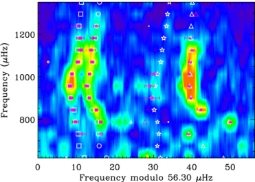
By looking at the échelle diagram (Fig.6), we notice an avoided crossing, corresponding to the presence of a mixed mode (e.g.
Fig. 5. Upper panel: PSD of HD 169392 in the p-mode region at full resolution (grey) and smoothed over 15-bin wide boxcar (black). The red line corresponds to the fitted spectrum from refit after the frequency comparison stage. Lower panel: power spectral density for the p-mode region divided by the fitted model at full resolution (grey) and smoothed over 15 bins (black). Regions highlighted in green cover the regions corresponding to the harmonics of the CoRoT orbital period such that ν= (n × 161.7) ± (m × 11.5) µHz, where n and m are integers. The arrows show the positions where we would expect `= 3 modes.
Fig. 6. Échelle diagram of the CoRoT target, HD 169392A, with the minimal (close pink symbols) and maximal (open and close pink sym-bols) lists of frequencies, and the frequencies from the best-fit model of AMP (white symbols): `= 0 (circles), ` = 1 (triangles), ` = 2 (squares), and `= 3 (stars) as in Sect. 7.2. The pink triangles without uncertainties correspond to the mixed modes (`= 1) mentioned in Sect. 7.3.
Osaki 1975;Aizenman et al. 1977;Deheuvels & Michel 2011). The frequency pattern is affected by the coupling of the pres-sure wave in the outer convective region with a gravity wave in the radiative interior. Hence, we can use the formalism devel-oped for mixed modes in giants (Mosser et al. 2012) to describe this pattern.
Table 6. Mixed-mode parameters.
Asymptotic p modes
Pressure phase offset εp 1.17 ± 0.02
Small separation d01 0.03 ± 0.02
Curvature α 0.0029 ± 0.0008
Asymptotic g modes
Gravity period spacing ∆Π1 476.9 ± 4.3 s
Gravity phase offset εg 0.07 ± 0.03
Mixed modes
Coupling q 0.098 ± 0.005
For p modes, the second-order correction of the asymptotic relation is related by a curvature term α:
νnp,`= np+ ` 2 + εp− d0`+ α 2[np− nmax] 2 ! ∆ν, (3)
where εp is the pressure phase offset, d0`accounts for the small
separation, and nmax= νmax/∆ν. The g modes are reduced to the
first-order term:
Png,`=1= (|ng|+ εg)∆Π1, (4)
where ng is the gravity radial order, εgthe gravity phase offset,
and∆Π1the gravity period spacing of dipole modes.
The coupling of the p and g waves is then expressed by a sin-gle constant (Mosser et al. 2012). Table6shows the asymptotic parameters used for the fit. Compared to modes in giants that have very large gravity orders (in absolute value), mixed modes
A&A 549, A12 (2013)
Fig. 7.Large separation as a function of frequency for `= 0, 1 and 2. The dashed line represents the mean large separation of the radial modes. The red squares at low- and high frequency represent the values obtained using the modes of the maximal list.
in a subgiant with∆ν ' 56 µHz have small |ng|. Therefore, we
cannot consider the asymptotic constant εgto be 0.
The best fit of the radial ridge, obtained from a global agree-ment over nine orders, is provided with ∆ν = 56.3 µHz and εp = 1.17. We then infer a gravity period spacing of
approx-imately 476.9 ± 4.3 s, with a precision limited by the uncer-tainty on the unknown gravity offset. Best fits are obtained with εg = 0.07 ± 0.03. In all cases, the coupling is small: q =
0.098 ± 0.005. Two mixed modes are reported at 816 and 1336 µHz with gravity orders of −2 and −1, respectively, cor-responding to the period of g modes (the avoided crossing), Pg= (|ng|+ 1/2 + εg)∆Π1(Goupil et al., in prep.). These mixed
modes bring strong constraints on the age of a star as the cou-pling between the p- and g-mode cavities changes quickly with stellar age, yielding strong constraints on the age of the star (e.g.
Christensen-Dalsgaard 2004;Metcalfe et al. 2010;Mathur et al. 2012). The presence of the mixed modes in HD 169392A indi-cates that this star is quite evolved.
Unfortunately, none of these two modes were fitted by the nine teams. The peak at 816 µHz is surrounded by the orbital harmonics and without a proper modelling of these peaks, it is not possible to fit the mixed mode. The high-frequency mixed mode at 1336 µHz has too weak a signal to be fitted.
7.4. Frequency differences
We fitted the frequencies of the `= 0 modes against the order n and according to Eq. (3), the slope is the mean large frequency separation. We obtained h∆νi = 55.98 ± 0.05 µHz, which agrees with the value obtained from the global techniques (see Sect.4) and the mixed-mode asymptotic fit (Sect. 7.3). The variation of the mean large separation is shown in Fig. 7. We notice the dip for the modes `= 1, due to the avoided crossing mentioned above. The low oscillation we observe is typical of the signature we can have for the second helium ionisation zone below the stellar surface. We would need more modes to be able to extract the position this ionisation zone.
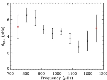
We also computed the variation of the small separation be-tween ` = 0 and 2 following Roxburgh & Vorontsov (2003), which is shown in Fig.8. The small separation presents a gen-eral decreasing trend (with a slope of −0.007), which is very
Fig. 8.Small separation, δ02, as a function of frequency. The red squares
at low- and high frequency represent the values obtained using the modes of the maximal list.
similar to what we observe on the Sun. The mean value is around 4.14 µHz. This value perfeclty fits the CD diagram presented by
White et al.(2011) where for subgiants the small separation is approximately the same as for stars with very different masses. 7.5. Linewidths
The linewidths of the modes (Γ`,n) as measured in the power
spectrum are related to their lifetimes (τ`,n) as indicated next for a mode of degree `= 0 and order n:
τ0,n= (πΓ0,n)−1, (5)
The results from the MCMC method, which fitted a single linewidth for ` = 0, 1, and 2 modes per order, are given in Table7and are represented in Fig.9. We note that the trend is rather flat with a median value of 1.8 µHz, with a little increase with frequency. The first and last points were obtained with the frequency of the maximal list of modes. This behaviour is sim-ilar to the one found in the Sun in the plateau region and the higher frequencies. We also observe a low oscillation followed by a small increase of the linewidth, which is also seen in other G-type stars observed by CoRoT (e.g.Deheuvels et al. 2010;
Ballot et al. 2011b).
There have been several projects that aimed to show a power-law dependence of the linewidths on the effective temperature of the star asΓ ∼ Ts
eff.Chaplin et al. (2009) derived a
relation-ship indicating that the mean linewidth should scale as T4 eff for
temperatures ranging between 6800 K and 5300 K. Later work byBaudin et al.(2011) using five main-sequence stars observed by CoRoT plus the Sun re-evaluated the exponent to be 16 ± 2. Recently,Appourchaux et al.(2012a) used an analysis of 42 cool main-sequence stars and subgiants observed by Kepler to refine the expression toΓ ∼ T15.5
eff . For HD 169392, we measure the
linewidth at maximum height as 1.41 µHz (` = 0, n = 18), a value that agrees very well with Fig.2ofAppourchaux et al.
(2012a) using Teff = 5885 K and with the theoretical
compu-tation byBelkacem et al.(2012). Finally,Corsaro et al.(2012) analysed the linewidth of red-giant stars in clusters and found that by taking into account main-sequence and subgiant stars, Γ varies exponentially with Teff, which gives 1.66 µHz, still in
Fig. 9. Linewidths of `= 0 modes as a function of frequency. Same legend as in Fig.8. A single linewidth was fitted for each order.
7.6. Amplitudes
From the heights and linewidths of the modes in the power spec-trum, we can compute the rms amplitude of each mode accord-ing to the followaccord-ing expression:
A`,n= r πΓ`,nH`,n
2 , (6)
whereΓ`,nis the width of the mode (`, n) and H`,nis the height of that mode in a single-sided power spectrum (hence the factor 2 in the numerator). The values obtained are listed in Table7and are shown in Fig.10. We can see the profile of the p-mode bump. The maximum mode amplitude is 3.82 ± 0.30 ppm, which agrees with the value obtained in Sect. 4.1 (3.61 ± 0.35 ppm). Owing to the imperfect observational window (with a duty cycle of ∼0.83), there is a substantial leakage of mode power in small aliases. We corrected the amplitude for this effect, which led to an observed value of 4.12 ± 0.32 ppm. To take into account the response function of CoRoT, we converted the amplitude to the bolomet-ric one by computing Rosc= 7.87 and R`=0 = 4.44 (seeMichel et al. 2009, for details), which gives the bolometric correction cbol = 0.90 ± 0.01. Finally, since HD 169392 is a binary, a part
of the observed total flux comes from the secondary component. With the magnitude quoted in Sect. 1, we find LA/LB = 3.9,
which allows us to conclude that ∼20% of the flux is dimmed by the second component. Therefore, the final value for the maxi-mal amplitude of the modes is Aobsmax= 4.45 ± 0.34 ppm.
Several expressions have been developed the last few years to compute the maximum amplitude of the modes. According toSamadi et al.(2007b), the theoretical value of the maximum amplitude is obtained with
Amax= L/L M/M !s s 5777 Teff A ,max, (7) with s = 0.7 and according to Michel et al.(2009), A ,max =
2.53 ± 0.11 ppm (in rms). Using the values of R and M from the AMP model (see Sect. 8), we obtain 6.02 ± 0.60 ppm.
We computed the theoretical value with the updated scaling relation derived byKjeldsen & Bedding(2011), which depends on the lifetime of the modes, τosc:
Amax∝
Lτ0.5 osc
(M/M )1.5Te2.25ff +r
, (8)
Fig. 10.Amplitude of `= 0 modes as a function of frequency. Same legend as in Fig.8.
We took r = 1.5 as adopted byMichel et al. (2008) and ob-tain 4.32 ± 1.10 ppm, which is much closer to the observed amplitude.
Huber et al. (2011) used several hundred red giants and main-sequence stars to derive an empirical relation, which is slightly different from the previous one but similar to the re-sults obtained from red giants observed in clusters (Stello et al. 2011a). This relation is more dependent on the mass of the star: Amax= (L/L )s (M/M )t 5777 Teff A ,max, (9) with s= 0.838, t = 1.32, and A ,max= 2.53 ± 0.11 ppm (in rms),
leading to 6.58 ± 0.79 ppm forHuber et al.(2011).Stello et al.
(2011a) found slightly different parameters: s = 0.95 and t = 1.8 (in the adiabatic case), which gives Amax= 7.21 ± 0.92 ppm.
The observed value is at the lower limit of the theoretical ones within 3-σ for modellings in Eqs. (7) and (9) and agrees within 1-σ with the prediction from Eq. (8).
7.7. Relative visibilities
Accurate estimation of the relative visibilities of non-radial modes is important for our knowledge of the physics of the stel-lar atmospheres because the visibilities depend on the stelstel-lar limb darkening and the observed wavelengths. Although well-defined in the Sun at different heights in the solar photosphere (Salabert et al. 2011), the measurements of relative visibilities are more critical for other stars due to lower S/N and shorter time series. Nevertheless, the mode visibilities were successfully determined in two of the CoRoT stars: HD 52265 (Ballot et al. 2011b) and HD 49385 (Deheuvels et al. 2010). The measured visibilities quantitatively agree well with theoretical calculations of limb-darkening functions fromBallot et al.(2011a), who also showed a dependence on Teff.
Estimates of the relative visibilities, V2
l, of ` = 1, 2, and
3 modes were obtained for HD 169392A. Consistent values within the error bars were obtained among the different peak-fitting techniques. Some tests using different inclination angles and rotational splittings showed that the uncovered visibilities give similar results within the uncertainties. The relative visibil-ity of the modes `= 1, 2, and 3 measured by the MCMC analysis are given in Table8, as well as the median values of their distri-butions and associated 1-σ values.
A&A 549, A12 (2013) Table 8. Medians and standard deviations for the inclination angle (i),
the rotational splitting (νs), the projected splitting (νssin i), and the
rel-ative visibilities of the `= 1, 2, and 3 modes (Vl=1, Vl=2, Vl=3) obtained from MCMC. i(◦ ) νs(µHz) νssin i (µHz) Vl2=1 Vl2=2 Vl2=3 Median 36 0.62 0.38 1.41 0.68 0.15 −σ 20 0.23 0.16 0.17 0.11 0.07 +σ 36 0.59 0.11 0.20 0.11 0.08
Notes. These statistical informations are deduced from the joint-probability density function of the inclination/splitting and from the probability density function for the other parameters.
7.8. Splitting and inclination angle
We also checked the extent to which the estimated frequencies, amplitudes, and linewidths were independent of the assumed an-gle of inclination.
Multiple fits were performed for a fixed rotational split-ting and a range of fixed angles, using the MCMC method. An additional check was performed by looking at the correlation map between width, inclination angle, and splittings from the MCMC technique. The mode frequencies returned by the vari-ous fits were found to be independent of the angle used, at the level of precision of the data. The mode linewidths and ampli-tudes showed a weak dependence on the angle of inclination and the splittings at extreme values of the inclination. But any changes were at a much lower level than the 1-σ error bars when the angle was in the range 15◦ ≤ i ≤ 85◦, i.e., the limits
sug-gested by MCMC results.
Figure 11 shows the correlation map of the splitting and the inclination (two-dimensional probability density function). We notice two maxima of almost equally high probabil-ity into the joint-posterior probabilprobabil-ity densprobabil-ity function. This bi-modality suggests that two different values for the joint-parameters are possible. However, the two solutions are com-patible within 2σ and therefore are not statistically different (cf. Table 8). To achieve a more stringent determination, one would need additional constraints, such as the signature of the surface rotation, which unfortunately cannot be detected in the present dataset (see Sect.5.2).
The product of the splitting and angle parameters, which gives the so-called projected splitting, νssin i, is well-defined,
as seen by the curved ridge and the uncertainties presented in Table 8. However, as anticipated by Ballot et al.(2006), a ro-bust estimation of the individual parameters is hampered by two competing solutions, the first with relatively low angle and high splitting, and the second with high angle and lower splitting. Our inability to discern between the two solutions prevents us from reporting final values for each parameter.
8. Modelling HD 169392A
With the spectroscopic and asteroseismic information derived in the previous sections, we modelled HD 169392A using the Asteroseismic Modeling Portal (AMP, Metcalfe et al. 2009). This is a genetic algorithm that aims at optimising the match between the observed and the modelled frequencies of the star in addition to the spectroscopic constraints. The models are computed by the Aarhus STellar Evolution Code (Christensen-Dalsgaard 2008), which is also used to build the standard model of the Sun. It includes the OPAL 2005 equa-tion of state (Rogers & Nayfonov 2002) and the most recent
Fig. 11.Correlation map between rotational splitting and inclination. The red (yellow) region corresponds to the 1-σ (2-σ) confidence area.
OPAL opacities (Iglesias & Rogers 1996) associated with the low-temperature opacity table ofAlexander & Ferguson(1994). Finally, the convection is treated according to the mixing-length theory (Böhm-Vitense 1958), and diffusion and gravitational set-tling of helium follow the prescription byMichaud & Proffitt
(1993). A surface correction was applied to the frequencies fol-lowing the prescription byKjeldsen et al.(2008b). AMP has al-ready modelled a large number of stars (e.g.Metcalfe et al. 2010;
Mathur et al. 2012;Metcalfe et al. 2012) for a given physics. For the observables, we used the spectroscopic constraints from Table 1 and the mode frequencies from the minimal list (Table5). The best-fit model obtained has a χ2 of 1.02. Since
seismic and spectroscopic observables are used, we also com-puted two separate normalised χ2: χ2
spec= 0.22 and χ2seis= 1.43.
The χ2
spec agrees well for the observables and the best-fit
model. In Fig. 6, the model frequencies are superimposed on the échelle diagram obtained with CoRoT data, and we can see that the best-fit model frequencies match the observations well. We also notice that the maximal list frequencies, including the ` = 3 modes, are well-reproduced by the model, suggesting that these frequencies probably correspond to a real signal.
We obtained a mass of M= 1.15 ± 0.01 M , a radius of R=
1.88 ± 0.02 R , and an age τ= 4.33 ± 0.12 Gyr. The
uncer-tainties come from estimated errors on the observables but do not include uncertainties in the surface layer correction, and the physics of stellar models.
Using the parallax π= 13.82 ± 1.2 mas, we obtained a lumi-nosity L= 4.16 ± 0.6 L while the value from the best-fit model
of AMP is 4.18 ± 0.01 L , a very good agreement.
We also followed the methodology developed by Silva Aguirre et al.(2012) to couple theCasagrande et al.(2010) im-plementation of the infrared flux method (IRFM) with an astero-seismic analysis. This technique provides results using both the direct and grid-based methods, as well as a determination of the distance to the target. The results completely agree with those from the AMP analysis for log g and Teff(see Table9). The mass
and radius agree with the first method to within 1σ and with the second one to within 2σ. The distance determined by these tech-niques is d= 70 ± 5.3 pc, in excellent agreement with parallax measurements.
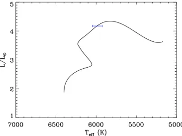
The best-fit model of AMP confirms that this is indeed a sub-giant that has exhausted its central hydrogen and has no convec-tive core. As seen on the HR diagram with the evolutionary track
Table 9. Modeling results from AMP, direct method+ IRFM, and grid-based method + IRFM.
Method M(M ) R(R ) τ (Gyr) log g (dex) Teff(K) L/L
AMP 1.15 ± 0.01 1.88 ± 0.02 4.33 ± 0.12 3.95 ± 0.01 6016 ± 5 4.18 ± 0.01 Direct method+ IRFM 1.30 ± 0.23 1.93 ± 0.13 – 3.97 ± 0.02 6002 ± 77 4.45 ± 0.67 Grid-based method+ IRFM 1.25+0.05−0.03 1.96 ± 0.02 – 3.95 ± 0.01 6002 ± 77 4.51 ± 1.04 Notes. The uncertainties for the AMP best fit model are the internal errors.
Fig. 12.Evolutionary track computed by AMP and position of the best-fit model with the spectroscopic uncertainty (blue symbol).
for this model (Fig.12), it has not yet started to ascend the red giant branch.
9. Conclusion
In the present analysis we have derived the fundamental param-eters of the two components of the binary system HD 169392 using HARPS observations. We obtained very close values of metallicity for the two components. This is quite similar to the results observed for other binary systems (e.g. 16 CygMetcalfe et al. 2012), suggesting that the A and B components were formed from the same cloud of gas and dust. Neither of the two components has significant amount of Li.
We were unable to detect a significant seismic signature of the B component from an analysis of the 91 days of CoRoT ob-servations. This result agrees with the low detectability proba-bility of 2% for the B component.
We determined the global parameters of the modes of HD 169392A, which led to h∆νi of 56.98 ± 0.05 µHz and νmax
of 1030 ± 55 µHz, making this star very similar to another CoRoT target, HD 49385 (Deheuvels et al. 2010).
Nine groups reported p-mode parameters. The comparison of the results led to a minimal and maximal lists of frequencies. Some significant power was found in the region where we would expect `= 3 modes. We fitted the ` = 0, 1, 2, and 3 modes to-gether with the MCMC technique and obtained that three modes ` = 3 are significant according to the a posteriori probability. We analysed the mixed modes of the star using their asymp-totic properties and detected two avoided crossings at 816 µHz and 1336 µHz. From these avoided crossings, we derived the gravity spacing ∆Π1 = 477 ± 5 s. We conclude that this star is
quite evolved but not yet on the red-giant branch.
We derived the amplitude of the modes that is smaller than the predicted amplitudes within 1- to 3-σ depending on the the-oretical formula applied. The linewidths of the modes obtained are consistent with the dependence on effective temperature de-rived byAppourchaux et al.(2012a) andCorsaro et al.(2012).
The study of the splittings and inclination angles led to two possible solutions. We obtained either an inclination angle of 20−40◦with splittings of 0.4−1.0 µHz, or an inclination angle
of 55−85◦and splittings of 0.2−0.5 µHz. We note that no clear signature of the surface rotation was detected and in the absence of additional constraints, the significant correlation between the splitting and the inclination angle prevents us from constraining them more precisely.
The global parameters of the modes allowed us to give a first estimate of the mass and radius of the star using scaling rela-tions based on solar values: 1.34 ± 0.26 M and 1.97 ± 0.19 R .
A more thorough modelling with AMP, based on the match of the individual mode frequencies and the spectroscopic parame-ters obtained in this work, provided M= 1.15 ± 0.01 M , a
ra-dius of R= 1.88 ± 0.02 R , and an age τ= 4.33 ± 0.12 Gyr.
Acknowledgements. The authors thank V. Silva Aguirre, L. Cassagrande, and T. S. Metcalfe for useful comments and discussions. This work was par-tially supported by the NASA grant NNX12AE17G. The CoRoT space mis-sion has been developed and is operated by CNES, with contributions from Austria, Belgium, Brazil, ESA (RSSD and Science Program), Germany and Spain. R.A.G. acknowledges the support given by the French PNPS program. R.A.G. and S.M. acknowledge the CNES for the support of the CoRoT ac-tivities at the SAp, CEA/Saclay. D.S. acknowledges the support from CNES. S.H. acknowledges financial support from the Netherlands Organization for Scientific Research (NWO). NCAR is supported by the National Science Foundation. L.M., E.P., and M.R. acknowledge financial support from the PRIN-INAF 2010 (Asteroseismology: looking inside the stars with space-and ground-based observations). K.U. acknowledges financial support by the Spanish National Plan of R&D for 2010, project AYA2010-17803. C.R., S.B.F. and T.R.C. wish to acknowledge financial support from the Spanish Ministry of Science and Innovation (MICINN) under the grant AYA2010-20982-C02-02. W.J.C., Y.E., I.W.R., and G.A.V. acknowledge support from the UK Science and Technology Facilites Council (STFC). The research lead-ing to these results has received fundlead-ing from the European Community’s Seventh Framework Programme (FP7/2007−2013) under grant agreement No. 269194 (IRSES/ASK). Computational time on Kraken at the National Institute of Computational Sciences was provided through NSF TeraGrid allo-cation TG-AST090107.
References
Aizenman, M., Smeyers, P., & Weigert, A. 1977, A&A, 58, 41 Alexander, D. R., & Ferguson, J. W. 1994, ApJ, 437, 879
Anderson, E. R., Duvall, Jr., T. L., & Jefferies, S. M. 1990, ApJ, 364, 699 Appourchaux, T. 2008, Astron. Nachr., 329, 485
Appourchaux, T. 2011 [arXiv:1103.5352]
Appourchaux, T., Gizon, L., & Rabello-Soares, M.-C. 1998, A&AS, 132, 107 Appourchaux, T., Michel, E., Auvergne, M., et al. 2008, A&A, 488, 705 Appourchaux, T., Benomar, O., Gruberbauer, M., et al. 2012a, A&A, 537, A134 Appourchaux, T., Chaplin, W. J., García, R. A., et al. 2012b, A&A, 543, A54 Auvergne, M., Bodin, P., Boisnard, L., et al. 2009, A&A, 506, 411
Baglin, A., Auvergne, M., Boisnard, L., et al. 2006, in COSPAR, Plenary Meeting, 36th COSPAR Scientific Assembly, 36, 3749
Ballot, J., García, R. A., & Lambert, P. 2006, MNRAS, 369, 1281 Ballot, J., Barban, C., & van’t Veer-Menneret, C. 2011a, A&A, 531, A124 Ballot, J., Gizon, L., Samadi, R., et al. 2011b, A&A, 530, A97
A&A 549, A12 (2013)
Barban, C., Deheuvels, S., Baudin, F., et al. 2009, A&A, 506, 51 Basu, S., Grundahl, F., Stello, D., et al. 2011, ApJ, 729, L10 Baudin, F., Barban, C., Belkacem, K., et al. 2011, A&A, 529, A84 Belkacem, K., Goupil, M. J., Dupret, M. A., et al. 2011, A&A, 530, A142 Belkacem, K., Dupret, M. A., Baudin, F., et al. 2012, A&A, 540, L7 Benomar, O. 2008, Commun. Asteroseismol., 157, 98
Benomar, O., Bedding, T. R., Stello, D., et al. 2012, ApJ, 745, L33 Böhm-Vitense, E. 1958, ZAp, 46, 108
Borucki, W. J., Koch, D., Basri, G., et al. 2010, Science, 327, 977
Brown, T. M., Gilliland, R. L., Noyes, R. W., & Ramsey, L. W. 1991, ApJ, 368, 599
Bruntt, H., Bedding, T. R., Quirion, P.-O., et al. 2010, MNRAS, 405, 1907 Bruntt, H., Basu, S., Smalley, B., et al. 2012, MNRAS, 423, 122 Campante, T. L., Handberg, R., Mathur, S., et al. 2011, A&A, 534, A6 Casagrande, L., Ramírez, I., Meléndez, J., Bessell, M., & Asplund, M. 2010,
A&A, 512, A54
Catala, C., Poretti, E., Garrido, R., et al. 2006, in ESA SP 1306, eds. M. Fridlund, A. Baglin, J. Lochard, & L. Conroy, 329
Chaplin, W. J., Houdek, G., Karoff, C., Elsworth, Y., & New, R. 2009, A&A, 500, L21
Chaplin, W. J., Kjeldsen, H., Bedding, T. R., et al. 2011a, ApJ, 732, 54 Chaplin, W. J., Kjeldsen, H., Christensen-Dalsgaard, J., et al. 2011b, Science,
332, 213
Christensen-Dalsgaard, J. 2002, Rev. Mod. Phys., 74, 1073 Christensen-Dalsgaard, J. 2004, Sol. Phys., 220, 137 Christensen-Dalsgaard, J. 2008, Ap&SS, 316, 13
Christensen-Dalsgaard, J., & Thompson, M. J. 2011, in Astrophysical Dynamics: From Stars to Galaxies, Proc. of the International Astronomical Union, IAU Symp., 271, 32
Corsaro, E., Stello, D., Huber, D., et al. 2012, ApJ, 757, 190 Creevey, O. L., Do˘gan, G., Frasca, A., et al. 2012, A&A, 537, A111 Deheuvels, S., & Michel, E. 2011, A&A, 535, A91
Deheuvels, S., Bruntt, H., Michel, E., et al. 2010, A&A, 515, A87 Duncan, D. K. 1984, AJ, 89, 515
Escobar, M. E., Théado, S., Vauclair, S., et al. 2012, A&A, 543, A96
Fletcher, S. T., Broomhall, A.-M., Chaplin, W. J., et al. 2011, MNRAS, 413, 359 García, R. A., Régulo, C., Samadi, R., et al. 2009, A&A, 506, 41
García, R. A., Hekker, S., Stello, D., et al. 2011, MNRAS, 414, L6 Gaulme, P., Appourchaux, T., & Boumier, P. 2009, A&A, 506, 7 Gaulme, P., Vannier, M., Guillot, T., et al. 2010, A&A, 518, L153 Goldreich, P., & Keeley, D. A. 1977, ApJ, 212, 243
Gough, D. O., Kosovichev, A. G., Toomre, J., et al. 1996, Science, 272, 1296 Gould, B. A. 1855, AJ, 4, 81
Gustafsson, B., Edvardsson, B., Eriksson, K., et al. 2008, A&A, 486, 951 Handberg, R., & Campante, T. L. 2011, A&A, 527, A56
Harvey, J. 1985, in Future Missions in Solar, Heliospheric & Space Plasma Physics, eds. E. Rolfe, & B. Battrick, ESA SP, 235, 199
Hekker, S., Broomhall, A., Chaplin, W. J., et al. 2010a, MNRAS, 402, 2049 Hekker, S., Debosscher, J., Huber, D., et al. 2010b, ApJ, 713, L187 Hekker, S., Elsworth, Y., De Ridder, J., et al. 2011, A&A, 525, A131 Holmberg, J., Nordström, B., & Andersen, J. 2007, A&A, 475, 519 Howell, S. B., Rowe, J. F., Bryson, S. T., et al. 2012, ApJ, 746, 123 Huber, D., Bedding, T. R., Stello, D., et al. 2011, ApJ, 743, 143 Iglesias, C. A., & Rogers, F. J. 1996, ApJ, 464, 943
Israelian, G., Santos, N. C., Mayor, M., & Rebolo, R. 2004, A&A, 414, 601 Kjeldsen, H., & Bedding, T. R. 1995, A&A, 293, 87
Kjeldsen, H., & Bedding, T. R. 2011, A&A, 529, L8
Kjeldsen, H., Bedding, T. R., Arentoft, T., et al. 2008a, ApJ, 682, 1370 Kjeldsen, H., Bedding, T. R., & Christensen-Dalsgaard, J. 2008b, ApJ, 683, L175 Koch, D. G., Borucki, W. J., Basri, G., et al. 2010, ApJ, 713, L79
Kupka, F., Piskunov, N., Ryabchikova, T. A., Stempels, H. C., & Weiss, W. W. 1999, A&AS, 138, 119
Mathur, S., García, R. A., Catala, C., et al. 2010a, A&A, 518, A53 Mathur, S., García, R. A., Régulo, C., et al. 2010b, A&A, 511, A46 Mathur, S., Handberg, R., Campante, T. L., et al. 2011a, ApJ, 733, 95 Mathur, S., Hekker, S., Trampedach, R., et al. 2011b, ApJ, 741, 119 Mathur, S., Metcalfe, T. S., Woitaszek, M., et al. 2012, ApJ, 749, 152 Mayor, M., Pepe, F., Queloz, D., et al. 2003, The Messenger, 114, 20
Mazumdar, A., Michel, E., Antia, H. M., & Deheuvels, S. 2012, A&A, 540, A31 Metcalfe, T. S., Creevey, O. L., & Christensen-Dalsgaard, J. 2009, ApJ, 699, 373 Metcalfe, T. S., Monteiro, M. J. P. F. G., Thompson, M. J., et al. 2010, ApJ, 723,
1583
Metcalfe, T. S., Chaplin, W. J., Appourchaux, T., et al. 2012, ApJ, 748, L10 Michaud, G., & Proffitt, C. R. 1993, in Inside the Stars, eds. W. W. Weiss, & A.
Baglin, IAU Colloq., 137, ASP Conf. Ser., 40, 246
Michel, E., Baglin, A., Auvergne, M., et al. 2008, Science, 322, 558 Michel, E., Samadi, R., Baudin, F., et al. 2009, A&A, 495, 979 Mosser, B., & Appourchaux, T. 2009, A&A, 508, 877
Mosser, B., Baudin, F., Lanza, A. F., et al. 2009a, A&A, 506, 245 Mosser, B., Michel, E., Appourchaux, T., et al. 2009b, A&A, 506, 33 Mosser, B., Goupil, M. J., Belkacem, K., et al. 2012, A&A, 540, A143 Nordström, B., Mayor, M., Andersen, J., et al. 2004, A&A, 418, 989 Osaki, J. 1975, PASJ, 27, 237
Peirce, B. 1852, AJ, 2, 161
Piau, L., Turck-Chièze, S., Duez, V., & Stein, R. F. 2009, A&A, 506, 175 Poretti, E., Rainer, M., Mantegazza, L., et al. 2012 [arXiv:1202.3542] Press, W. H., Teukolsky, S. A., Vetterling, W. T., & Flannery, B. P. 1992,
Numerical recipes in FORTRAN, The art of scientific computing, 2nd edn. (Cambridge: University Press)
Rainer, M. 2003, Ph.D. Thesis, Università degli Studi di Milano Rogers, F. J., & Nayfonov, A. 2002, ApJ, 576, 1064
Roxburgh, I. W., & Vorontsov, S. V. 2003, A&A, 411, 215 Salabert, D., Fossat, E., Gelly, B., et al. 2004, A&A, 413, 1135 Salabert, D., Ballot, J., & García, R. A. 2011, A&A, 528, A25
Samadi, R. 2011, in The Pulsations of the Sun and the Stars, eds. J.-P. Rozelot, & C. Neiner (Berlin Springer Verlag), Lect. Notes Phys., 832
Samadi, R., Fialho, F., Costa, J. E. S., et al. 2007a [arXiv:astro-ph/0703354] Samadi, R., Georgobiani, D., Trampedach, R., et al. 2007b, A&A, 463, 297 Sato, K. H., Garcia, R. A., Pires, S., et al. 2010, ArXiv e-prints 1003.5178 Silva Aguirre, V., Casagrande, L., Basu, S., et al. 2012, ApJ, 757, 99
Sinachopoulos, D., Gavras, P., Dionatos, O., Ducourant, C., & Medupe, T. 2007, A&A, 472, 1055
Stello, D., Huber, D., Kallinger, T., et al. 2011a, ApJ, 737, L10 Stello, D., Meibom, S., Gilliland, R. L., et al. 2011b, ApJ, 739, 13 Struve, O., Franklin, K., & Stableford, C. 1955, ApJ, 121, 670
Unno, W., Osaki, Y., Ando, H., Saio, H., & Shibahashi, H. 1989, Nonradial os-cillations of stars
Uytterhoeven, K., Poretti, E., Rainer, M., et al. 2008, J. Phys. Conf. Ser., 118, 012077
van Leeuwen, F. 2007, A&A, 474, 653
Verner, G. A., Elsworth, Y., Chaplin, W. J., et al. 2011, MNRAS, 892 White, T. R., Bedding, T. R., Stello, D., et al. 2011, ApJ, 742, L3
Table 5. Minimal and maximal lists of frequencies for HD 169392 in µHz obtained from 91 days of CoRoT observations with MCMC. Order ` = 0 ` = 1 ` = 2 ` = 3 12 ... ... 743.22 ± 1.34a 13 748.35 ± 0.40a 770.96 ± 0.37 797.97 ± 0.76 ... 14 804.50 ± 0.35 838.21 ± 0.38 853.50 ± 0.85 ... 15 859.70 ± 0.38 886.83 ± 0.23 909.34 ± 0.46 ... 16 914.14 ± 0.27 940.52 ± 0.27 965.45 ± 0.41 930.52 ± 1.87b 17 969.77 ± 0.46 996.40 ± 0.32 1022.18 ± 0.27 986.08 ± 1.20b 18 1026.79 ± 0.27 1052.68 ± 0.20 1080.04 ± 0.44 1043.43 ± 1.23b 19 1083.77 ± 0.39 1109.19 ± 0.36 1137.05 ± 0.58 ... 20 1139.76 ± 0.42 1166.17 ± 0.34 1193.29 ± 0.97 ... 21 1196.71 ± 0.73 1221.76 ± 1.38 1248.79 ± 1.44a ... 22 1253.73 ± 0.75a ... ... ...
Notes.(a)Modes that belong to the maximal list.(b)Significant modes according to the MCMC method.
Table 7. Amplitudes and linewidths for all modes of Table5computed with the MCMC.
l n Linewidth (µHz) +σ −σ Amplitude (ppm) +σ −σ 0 13 0.80 1.02 0.64 1.63 0.33 0.32 0 14 1.39 0.65 0.62 2.40 0.30 0.32 0 15 1.35 0.39 0.30 2.83 0.29 0.27 0 16 1.30 0.63 0.43 2.81 0.31 0.26 0 17 2.37 0.61 0.52 3.82 0.30 0.29 0 18 1.00 0.57 0.27 3.72 0.36 0.37 0 19 2.01 0.77 0.54 3.39 0.31 0.29 0 20 1.97 0.58 0.47 3.23 0.24 0.25 0 21 4.14 1.53 1.18 2.54 0.25 0.27 0 22 1.27 1.35 0.77 1.36 0.29 0.36 1 13 0.80 1.02 0.64 1.94 0.38 0.40 1 14 1.39 0.65 0.62 2.84 0.37 0.37 1 15 1.35 0.39 0.30 3.37 0.32 0.31 1 16 1.30 0.63 0.43 3.35 0.34 0.32 1 17 2.37 0.61 0.52 4.53 0.34 0.33 1 18 1.00 0.57 0.27 4.40 0.42 0.38 1 19 2.01 0.77 0.54 4.04 0.33 0.33 1 20 1.97 0.58 0.47 3.83 0.31 0.31 1 21 4.14 1.53 1.18 3.02 0.31 0.33 2 12 0.80 1.02 0.64 1.34 0.28 0.27 2 13 1.39 0.65 0.62 1.96 0.28 0.27 2 14 1.35 0.39 0.30 2.33 0.25 0.24 2 15 1.30 0.63 0.43 2.32 0.25 0.23 2 16 2.37 0.61 0.52 3.13 0.25 0.25 2 17 1.00 0.57 0.27 3.04 0.32 0.29 2 18 2.01 0.77 0.54 2.79 0.26 0.26 2 19 1.97 0.58 0.47 2.64 0.27 0.24 2 20 4.14 1.53 1.18 2.08 0.23 0.25 2 22 1.69 1.42 0.91 0.99 0.27 0.29 3 16 1.30 0.63 0.43 0.65 0.07 0.06 3 17 2.37 0.61 0.52 0.89 0.07 0.07 3 18 1.00 0.57 0.27 0.86 0.08 0.09