HAL Id: hal-01678480
https://hal.archives-ouvertes.fr/hal-01678480
Submitted on 7 May 2018
HAL is a multi-disciplinary open access
archive for the deposit and dissemination of
sci-entific research documents, whether they are
pub-lished or not. The documents may come from
teaching and research institutions in France or
abroad, or from public or private research centers.
L’archive ouverte pluridisciplinaire HAL, est
destinée au dépôt et à la diffusion de documents
scientifiques de niveau recherche, publiés ou non,
émanant des établissements d’enseignement et de
recherche français ou étrangers, des laboratoires
publics ou privés.
COSMOS field: Multiwavelength counterparts and
redshift distribution
Drew Brisbin, Oskari Miettinen, Manuel Aravena, Vernesa Smolcic, Ivan
Delvecchio, Chunyan Jiang, Benjamin Magnelli, Marcus Albrecht, Alejandra
Munoz Arancibia, Herve Aussel, et al.
To cite this version:
Drew Brisbin, Oskari Miettinen, Manuel Aravena, Vernesa Smolcic, Ivan Delvecchio, et al.. An
ALMA survey of submillimeter galaxies in the COSMOS field: Multiwavelength counterparts and
redshift distribution. Astronomy and Astrophysics - A&A, EDP Sciences, 2017, 608,
�10.1051/0004-6361/201730558�. �hal-01678480�
September 11, 2017
An ALMA survey of submillimeter galaxies in the COSMOS field:
Multiwavelength counterparts and redshift distribution
Drew Brisbin
1, Oskari Miettinen
2, Manuel Aravena
1, Vernesa Smolˇci´c
2, Ivan Delvecchio
2, Chunyan Jiang
3, 4, 1,
Benjamin Magnelli
5, Marcus Albrecht
5, Alejandra Muñoz Arancibia
6, Hervé Aussel
7, Nikola Baran
2, Frank Bertoldi
5,
Matthieu Béthermin
8, 9, Peter Capak
10, Caitlin M. Casey
11, Francesca Civano
12, Christopher C. Hayward
13, 12, Olivier
Ilbert
8, Alexander Karim
5, Olivier Le Fevre
8, Stefano Marchesi
14, Henry Joy McCracken
15, Felipe Navarrete
5, Mladen
Novak
2, Dominik Riechers
16, Nelson Padilla
17, 18, Mara Salvato
19, Kimberly Scott
20, Eva Schinnerer
21, Kartik Sheth
22,
and Lidia Tasca
81 Núcleo de Astronomía, Facultad de Ingeniería y Ciencias , Universidad Diego Portales, Av. Ejército 441, Santiago, Chile 2 Department of Physics, Faculty of Science, University of Zagreb, Bijeniˇcka cesta 32, 10000 Zagreb, Croatia
3 CAS Key Laboratory for Research in Galaxies and Cosmology, Shanghai Astronomical Observatory, Nandan Road 80, Shanghai 200030, China
4 Chinese Academy of Sciences South America Center for Astronomy, 7591245 Santiago, Chile 5 Argelander-Institut für Astronomie, Universität of Bonn, Auf dem Hügel 71, D-53121 Bonn, Germany 6 Instituto de Física y Astronomía, Universidad de Valparaíso, Avda. Gran Bretana 1111, Valparaíso, Chile
7 Laboratoire AIM, IRFU/Service d’Astrophysique - CEA/DSM - CNRS - Université Paris Diderot, Bât. 709, CEA-Saclay, 91191 Gif-sur-Yvette Cedex, France
8 Aix Marseille Université, CNRS, LAM (Laboratoire d’Astrophysique de Marseille) UMR 7326, 13388, Marseille, France 9 European Southern Observatory, Karl-Schwarzschild-Str. 2, 85748 Garching, Germany
10 Department of Astronomy, California Institute of Technology, MC 249-17, 1200 East California Blvd, Pasadena, CA 11 Department of Astronomy, The University of Texas at Austin, 2515 Speedway Blvd Stop C1400, Austin, TX 78712, USA 12 Harvard-Smithsonian Center for Astrophysics, 60 Garden Street, Cambridge, MA 02138, USA
13 Center for Computational Astrophysics, Flatiron Institute, 162 Fifth Avenue, New York, NY 10010, USA
14 Department of Physics and Astronomy, Clemson University, Kinard Lab of Physics, Clemson, SC 29634-0978, USA 15 Sorbonne Universités, UPMC Univ Paris 06, UMR 7095, Institut d’Astrophysique de Paris, F-75005, Paris, France 16 Astronomy Department, Cornell University, 220 Space Sciences Building, Ithaca, NY 14853, USA
17 Instituto de Astrofísica, Universidad Católica de Chile, Av. Vicuna Mackenna 4860, 782-0436 Macul, Santiago, Chile 18 Centro de Astro-Ingeniería, Universidad Católica de Chile, Av. Vicuna Mackenna 4860, 782-0436 Macul, Santiago, Chile 19 Max-Planck-Institut für Extraterrestrische Physik (MPE), Postfach 1312, D-85741 Garching, Germany
20 National Radio Astronomy Observatory, 520 Edgemont Road, Charlottesville, VA 22903, USA 21 Max-Planck-Institut für Astronomie, Königstuhl, 17, 69117 Heidelberg, Germany
22 NASA Headquarters, 300 E. St SW, Washington DC 20546, USA September 11, 2017
ABSTRACT
We carried out targeted ALMA observations of 129 fields in the COSMOS region at 1.25 mm, detecting 152 galaxies at S/N≥5 with an average continuum RMS of 150 µJy. These fields represent a S/N-limited sample of AzTEC / ASTE sources with 1.1 mm S/N≥4 over an area of 0.72 square degrees. Given ALMA’s fine resolution and the exceptional spectroscopic and multiwavelength photometric data available in COSMOS, this survey allows us unprecedented power in identifying submillimeter galaxy counterparts and determining their redshifts through spectroscopic or photometric means. In addition to 30 sources with prior spectroscopic redshifts, we identified redshifts for 113 galaxies through photometric methods and an additional nine sources with lower limits, which allowed a statistically robust determination of the redshift distribution. We have resolved 33 AzTEC sources into multi-component systems and our redshifts suggest that nine are likely to be physically associated. Our overall redshift distribution peaks at z ∼2.0 with a high-redshift tail skewing the median redshift to ˜z=2.48±0.05. We find that brighter millimeter sources are preferentially found at higher redshifts. Our faintest sources, with S1.25mm<1.25 mJy, have a median redshift of ˜z=2.18±0.09, while the brightest sources, S1.25mm>1.8 mJy, have a median redshift of ˜z=3.08±0.17. After accounting for spectral energy distribution shape and selection effects, these results are consistent with several previous submillimeter galaxy surveys, and moreover, support the conclusion that the submillimeter galaxy redshift distribution is sensitive to survey depth.
Key words.
1. Introduction
Submillimeter bright galaxies (SMGs) represent a key popula-tion of star forming galaxies during the transipopula-tional epochs of
galaxy assembly and peak star formation. Better understanding the physical characteristics of SMGs and their role in galaxy evolution has been an ongoing goal in astronomy since their ini-tial discovery in low-resolution SCUBA observations (Smail et
al. 1997; Hughes et al. 1998; Barger et al. 1998). Infrared and submillimeter (submm) observations reveal that SMGs actively form stars at rates of approximately hundreds to thousands of M yr−1with correspondingly bright infrared luminosities&1012 L (Casey et al. 2014). Although they are similar in luminosity to local ultraluminous infrared galaxies (ULIRGs), local ULIRGs make up a very small fraction of the total star formation in the local universe and often have intense, compact star forming cores, whereas SMGs apparently compose a significant percent-age of the star formation rate density in the early Universe, and may often host more extended star formation (e.g., Menéndez-Delmestre et al. 2009; Magnelli et al. 2011; Hodge et al. 2015, 2016). This suggests that our understanding of SMGs is crucial to elucidating the evolution of galaxies in the early universe.
Early investigations of SMGs have been hindered by the large single-dish beam sizes of (sub-)mm observations and the difficulty in finding counterparts at other wavelengths to deter-mine galaxy properties and redshifts. A common procedure to pinpoint SMGs includes first surveying large areas of the sky us-ing bolometer cameras mounted on sus-ingle-dish (sub-)mm tele-scopes. The modest dish sizes of these telescopes (∼ 10 − 30m) imply that the typical beam size of such observations at wave-lengths between 870µm and 1.2 mm range approximately from 1100 to 3000. Secondly, since the number of sources in optical images within a typical submm beam element is typically more than five, it has been necessary to filter the possible counterpart identification by pre-selecting either faint radio or 24µm sources identified in deep radio interferometer or infrared maps (see Ivi-son et al. 2002, 2007; Bertoldi et al. 2007; Biggs et al. 2011; Smolˇci´c et al. 2012). The utility of radio pre-selection relies on the correlation between radio and infrared luminosities observed out to high redshifts (Helou et al. 1985; Carilli & Yun 1999; Yun et al. 2001), and assuming that both radio and infrared emission largely come from star formation activity. Finally, with the avail-able radio or 24 µm counterpart, a nearby optical to near-infrared source is identified. Using the multiwavelength photometry typ-ically available in the target submm fields, photometric redshifts are computed or optical-infrared follow-up spectroscopy is per-formed (e.g., Chapman et al. 2005). Alternatively, using various color-selection criteria shows promise as a method to identify potential optical SMG counterparts, especially in recent efforts using multiple color selections (Chen et al. 2016).
Due to the negative K correction in the Rayleigh-Jeans part of the dust spectral energy distribution (SED), the (sub)millimeter flux density remains almost constant with red-shift out to z ∼10 for a fixed IR luminosity. The radio and 24 µm emission, however, drop rapidly with redshift, becoming di ffi-cult to detect for most SMGs at z= 3. Therefore, apart from be-ing observationally expensive, the identification of SMGs based on radio or infrared selection fundamentally biases any study of SMGs to relatively low redshift, and raises the possibility of counterpart mis-identification by association with unassociated radio sources. Due to these limitations, direct (sub)millimeter in-terferometric follow-up of single-dish-selected sources has been used to directly find accurate SMG positions and counterparts (Downes et al. 1999, Iono et al. 2006; Younger et al. 2007, 2009; Aravena et al. 2010; Smolˇci´c et al. 2011, 2012a; Hodge et al. 2013; Miettinen et al. 2015a; Simpson et al. 2015).
Radio-identified SMGs typically lie at redshifts z ∼2-3 (e.g., Chapman et al. 2005; Wardlow et al. 2011). However, increas-ing evidence from time-consumincreas-ing follow-up observations and proper source identifications working against selection biases from faint optical and radio counterpart identification has sug-gested a possible high-redshift tail (z= 4 − 6) for this population
(Daddi et al. 2009a,b; Capak et al. 2008, 2011; Coppin et al. 2009; Knudsen et al. 2010; Smolˇci´c et al. 2011; Barger et al. 2012; Walter et al. 2012).
The Atacama Large Millimeter Array (ALMA) submm follow-up of 870 µm selected SMGs in the Extended Chandra Deep Field South (ECDFS), the ALESS survey, suggests that the SMG redshift distribution is similar to initial studies that were based on radio identification of SMGs, with a median redshift of 2.3-2.5 (Simpson et al. 2014; Fig. 2 therein), and a modest high-redshift tail at z&3.5. Several studies show evidence for the existence of an abundant z> 4 SMG population (Fig. 2; Capak et al. 2008, 2011; Schinnerer et al. 2008; Riechers et al. 2010, 2014; Aravena et al. 2010; Barger et al. 2012; Smolˇci´c et al. 2011, 2012a,b). The existence of a high-redshift tail has received support from ALMA spectroscopic follow up of SMGs discov-ered with the South Pole Telescope (SPT), with initial survey samples finding a median redshift of 3.5, and a later, expanded sample finding a median value of 3.9 (Vieira et al. 2013; Weiß et al. 2013; Strandet et al. 2016). Both the initial and the ex-panded samples were selected with relatively high 1.4 mm flux limits of 20 and 16 mJy, respectively, strongly biasing the sam-ples toward lensed systems and therefore systems at higher shifts. Although lensing bias corrections revise the median red-shift downward to z=3.1, this is still significantly higher than previous results (Strandet et al. 2016). Galaxies with very red SEDs, rising with wavelength out to 500 µm have also been shown to strongly correlate with galaxies at z&4, and their abun-dance in blind Herschel surveys similarly suggests a relatively abundant high-redshift tail (Riechers et al. 2013; Dowell et al. 2014; Asboth et al. 2016). The abundance of these high-redshift SMGs poses problems for cosmological models, given the di ffi-culty in creating large amounts of dust, stellar mass, and galaxy halos at early cosmic times (e.g. Baugh et al. 2005; Younger et al. 2007; Dwek et al. 2011; Hayward et al. 2011; Hayward et al. 2013b; Ferrara et al. 2016).
These results clearly show the need for an independent, quantitative study of SMGs to minimize biases from previous studies. These include general cosmic variance from small sam-ple sizes used in the mm follow-up of SMGs in COSMOS (Smolˇci´c et al. 2012a,b), the CO spectroscopy of H-ATLAS sources and the SPT SMGs (Harris et al. 2012; Weiß et al. 2013), and in the submm follow-up studies of SMGs in the ECDFS (Weiß et al. 2009); as well as potential bias from the selection waveband, as mm-selected sources may lie at higher redshift than submm-selected ones (Greve et al. 2008), and from UV-NIR and radio counterpart identification.
In this paper, we present counterparts and redshifts for a sam-ple of 129 SMGs that were initially discovered with the AzTEC camera on ASTE, and are now identified with high-resolution 1.25 mm ALMA imaging. Analyzed in conjunction with the most up-to-date panchromatic COSMOS data sets, we determine the multiwavelength counterparts and redshift distribution of our SMGs. In Sect. 2 we discuss our new observations and the an-cillary multiwavelength COSMOS data. In Sect. 3 we present the methods of counterpart detection, in Sect. 4 we present the methods of our redshift determinations, and in Sect. 5 we discuss the redshift distribution of our sample in comparison to other SMG studies. This paper is one in a series of works analyzing this sample. M. Aravena et al. (in prep) discusses the observa-tions, source catalog, and the flux distribution and clustering of the properties of sources revealed as multiples. C. Jiang et al. (in prep) analyzes the potential physical associations of those mul-tiples. Miettinen et al. (2017a) presents a spatial analysis of the radio emission and its implications for star formation. Miettinen
et al. (2017b) presents the multiwavelength SEDs of the sample and discusses the physical characteristics we determine based on these.
We adopt a flat ΛCDM cosmology, with ΩΛ=0.73, ΩM=0.27, and H0=72 km s−1Mpc−1.
2. Data
2.1. ALMA observations
We carried out targeted observations of 129 fields within the COSMOS region in cycle 2 ALMA operations at 1.25 mm (240 GHz). The observations were taken between 09 and 11 De-cember 2014, under good weather conditions. These fields were drawn from Aretxaga et al. (2011) to include a flux-limited sam-ple of AzTEC/ASTE sources with (deboosted) 1.1 mm flux den-sities ≥3.5 mJy covering the inner 0.72 square degrees of COS-MOS.
Band 6 continuum observations were taken with an aggre-gate bandwidth of 7.5 GHz centered on 240 GHz. Our observa-tions have fields of view of 2600. 3. We used the array in a rel-atively compact configuration using between 32 and 40 anten-nas, with a maximum baseline of ∼ 340 m. Initial continuum images were created from the visibilities by collapsing along the frequency axis and using natural weighting, resulting in a synthesized beam size of 1.6×0.93”. Sources which were de-tected in single pixels at significance levels above 5σ were then masked with tight boxes around the source, and cleaned down to a 2.5σ threshold. All fields reach a homogenous RMS of ∼150 µJy beam−1at an effective wavelength of 1.25 mm.
After cleaning the resulting images, 152 sources were de-tected at ≥5σ, within the beam width of the initial AzTEC obser-vations in each target field. Flux boosting due to the Eddington bias is expected to be very small at our achieved sensitivities and signal to noise. Simulation tests, performed by inserting false sources with signals in the range 2-40 σ confirm that at ≥5σ, flux boosting does not exceed map RMS. Therefore we did not apply any deboosting correction to our ALMA flux densities.
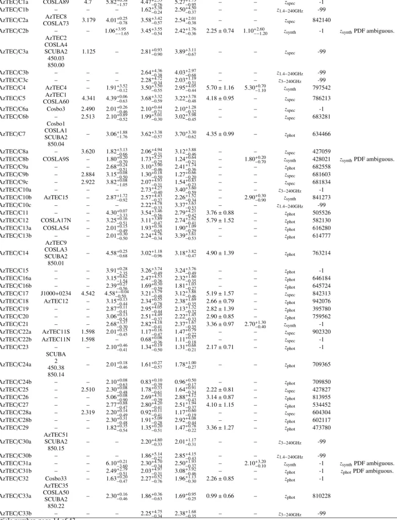
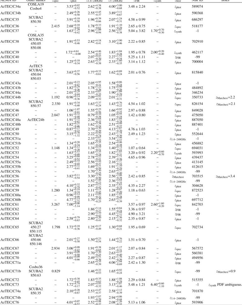
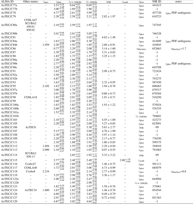
The sources, listed in Table 2, include 33 AzTEC sources that have been resolved into multiple components in the ALMA maps. These multi-component sources are noted by an alphabet-ical tag in order of their brightness (e.g., AzTEC/C1a is brighter than AzTEC/C1b). For an in-depth discussion of the ALMA ob-servations and source data see M. Aravena et al. (in prep). 2.2. UV-NIR
We used the latest COSMOS photometric catalog (COS-MOS2015 hereafter; Laigle et al. 2016), which includes pho-tometric measurements from the UV/optical to IR in over 20 bands, including 6 broad bands (B, V, g, r, i, z++), 12 medium bands, and 2 narrow bands, as well as Y, J, H and K s data from the UltraVISTA Data Release 2, new HyperSuprime-Cam Sub-aru Y band, and new SPLASH 3.6 and 4.5 µm Spitzer/Infrared Array Camera (IRAC) data (Sanders et al. 2007; Capak et al. 2007; McCracken et al. 2012; Ilbert et al. 2013; see Laigle et al. 2016 for details). The sources listed in the catalog were se-lected using the z++Y JHK s χ2 stacked mosaic generated after point-spread function homogenization across all bands (except GALEX and Spitzer/IRAC). For the homogenized bands aper-ture photometry is reported in the catalog, as well as the cor-rection of those to total magnitudes. The photometry in GALEX and Spitzer/IRAC bands was extracted using source-fitting tech-niques. Particular care was taken to robustly deblend the
lower-resolution IRAC photometry (using the tool IRACLEAN and prior positions extracted from the χ2 image; see Laigle et al. 2016 for details).
2.3. Spectroscopy
We also use the COSMOS spectroscopic redshift catalog (M. Salvato et al., in prep.), which compiles all available spec-troscopic redshifts, both available only to the COSMOS collab-oration and from the literature (zCOSMOS (Lilly et al. 2007, 2009), IMACS (Trump et al. 2007), MMT (Prescott et al. 2006), VIMOS Ultra Deep Survey (VUDS, Le Fèvre et al. 2015; Tasca et al. 2017), Subaru/FOCAS (T. Nagao et al., priv. comm.), and SDSS DR8 (Aihara et al. 2011)). In total, over 97,000 spectro-scopic redshifts are listed in the catalog, including 24 of our ALMA sources.
We also use the COSMOS spectroscopic redshift catalog (M. Salvato et al., in prep.), which compiles all available spec-troscopic redshifts, both available only to the COSMOS collab-oration and from the literature. This includes sources from the zCOSMOS bright survey, with sources selected based on an IAB magnitude < 22.5 (Lilly et al. 2007, 2009); the IMACS survey of x-ray and radio selected AGN with IAB < 24 (Trump et al. 2007); MMT which targeted quasars in the SDSS field with g band magnitudes <22.5 (Prescott et al. 2006); the VIMOS Ul-tra Deep Survey with sources selected for IAB < 25 (VUDS, Le Fèvre et al. 2015; Tasca et al. 2017); Subaru/FOCAS (T. Nagao et al., priv. comm.); and SDSS DR8 (Aihara et al. 2011)). In to-tal, over 97,000 spectroscopic redshifts are listed in the catalog, including 24 of our ALMA sources. At modest and high red-shifts (z&1) the various IABand optical selections will probe rest frame UV emission. Therefore these spectroscopic surveys may present a selection bias against high-redshift sources with ob-scured dusty star formation. This emphasizes the need to adopt alternate methods for determining redshifts when spectroscopic results are unavailable.
3. ALMA source counterparts and photometry
3.1. UV-NIR counterparts and photometry
We searched for UV-radio counterparts to our 152 ALMA sources by cross-matching our ALMA positions to the COS-MOS2015 catalog and the 3.6 µm Spitzer/IRAC selected catalog (Sanders et al. 2007) by relying on visual inspection of the opti-cal to NIR images. Visual inspection proved necessary to avoid potential mismatches from foreground sources. In total, we find counterparts for 135/152 (94%) sources. Out of these, 97 were drawn from the COSMOS2015 catalog. An additional 38 ALMA sources had blended catalog photometry (in some of the optical or NIR bands) or were not present in the COSMOS2015 cata-log. The latter occurs in case counterpart sources are present in bands blueward of z++ (e.g., i-band-detected sources; see e.g., AzTEC/C71b in Fig. 10) and/or redward of Ks (e.g., 3.6 µm; see e.g., AzTEC/C60b in Fig. 10), and not detected in the z++Y JHK stacked mosaic (see Laigle et al. 2016). For these 38 counter-parts we have specifically extracted the photometry in u, g, r, i, z++, UltraVISTA Y, J, H, K s, and Spitzer/IRAC 3.6, 4.5, 5.8 and 8.0 µm bands, and deblended where needed. This was done following the procedure described in detail in Smolˇci´c et al. (2012a), and further applied in Smolˇci´c et al. (2012b). Briefly, aperture and total magnitudes were first extracted for a sample of 100 randomly selected galaxies in the COSMOS field to cal-ibrate the photometry extraction, that is, match it to that in the
COSMOS2015 catalog. The same tool was then applied to ex-tract the photometry toward the 38 sources. Deblending was per-formed from case-to-case using prior positions, mostly fitting Gaussians to the blended sources, and subtracting the contam-inating source (see Smolˇci´c et al. 2012a for more details on the procedure). The extracted photometry for these sources is avail-able in the Appendix in Tavail-ables 3 and 4. All magnitudes are given in AB units.
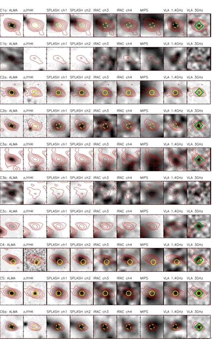
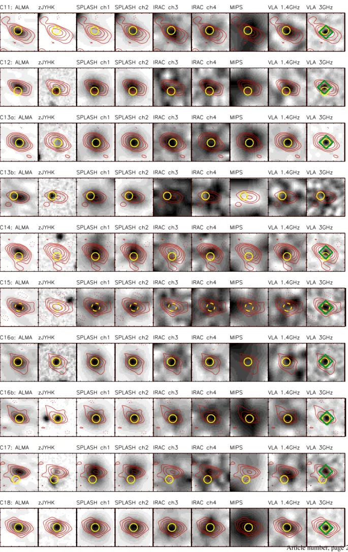
Zoomed images of the z++Y JHK s stacked, Spitzer/IRAC, and Spitzer/MIPS 24 µm (as well as 1.4 and 3 GHz radio maps – see Sect. 3.2) for each source, with ALMA contours overlaid and the counterpart indicated are shown in Fig. 10 in the Appendix. A list of the counterparts is given in Table 2.
The median separation between the ALMA position and that of the counterparts in the COSMOS2015 catalog for the 97 matches is 000. 25, with an interquartile range from 000. 11 to 000. 46, and a maximum separation of 000. 95. Out of the COSMOS2015 counterparts only 14/97 (14%) have separations larger than 000. 6.
3.2. Radio counterparts
We also cross-matched our ALMA catalog with an internal VLA-COSMOS 1.4 GHz catalog (see Schinnerer et al. 2007) as well as a 3 GHz catalog (Smolˇci´c et al. 2017).
Using search radii matching the mean resolutions in the ra-dio surveys (1.8 and 0.75” at 1.4 GHz and 3 GHz respectively) we find 48 counterparts at 1.4 GHz and 115 at 3 GHz (in to-tal 117 counterparts with either 1.4 GHz or 3 GHz counter-parts). This includes eight sources which do not have a UV-NIR counterpart. The median separation between the ALMA and 3GHz (S/N3GHz ≥ 5) radio positions is only 000. 12, with an in-terquartile range of 000. 07 − 000. 18, while for the 1.4 GHz sources (S/N3GHz ≥ 5) the median separation is 000. 20 and the interquar-tile range is 000. 13 − 000. 30.
The better agreement between the ALMA positions and the radio positions (compared to ALMA and the UV-NIR positions) is expected as i) the astrometric accuracy in the radio mosaic (000. 01 at S/N
3GHz> 20; Smolˇci´c et al. 2017) is much higher than that in the z++Y JHKstacked mosaic (better than 000. 15; Laigle et al. 2016), and ii) radio and mm wavelengths are both relatively unaffected by dust and are expected to trace roughly equivalent star-forming regions within the targeted galaxies. In practice, al-though the peak positions of radio and dust emissions appear to be coincident, the spatial scales appear different in the sense that the radio-emitting region of SMGs is on average about 2-4 times larger than that of the rest-frame FIR (see Miettinen et al. 2015b).
3.3. FIR - (sub-)mm counterparts and photometry
In addition to including flux densities from the 1.1 mm AzTEC observations (Aretxaga et al. 2011), we also cross-matched our ALMA sources with several submm and mm data sets including SCUBA 450 and 850 µm catalogs (Casey et al. 2013), LABOCA 870 µm (F. Navarrete, in prep.), SMA 890 µm data (Younger et al. 2007, 2009), MAMBO-2 1.2 mm (Bertoldi et al. 2007), and Herschel photometry from the Herschel Multitiered Extra-galactic Survey (HerMES) and PACS Evolutionary Probe (PEP) projects (Oliver et al. 2012 and Lutz et al. 2011, respectively). In cases of our ALMA multiple sources we used the low-resolution photometry from AzTEC and LABOCA to establish upper limits on flux densities. For photometry from SCUBA and MAMBO-2 we established upper limits only if the reported detections were
within one beam width of multiple ALMA sources (700, 1500, and 1100for SCUBA 450 µm, SCUBA 850 µm, and MAMBO-2 re-spectively) and otherwise associated the single dish photome-try with the ALMA source within half of a beam width. The Herschel photometry includes PACS and SPIRE photometry at 100,160, 250, 350, and 500 µm. Source photometry was ex-tracted and deblended according to techniques detailed in Mag-nelli et al. (2013), based both on our ALMA positions and 24 µm Spitzer sources as prior positions. For the AzTEC/C6 multi-SMG system we also included 870 µm ALMA data from Buss-mann et al. (2015).
4. Redshift determinations
4.1. Spectroscopic and photometric
In total we find spectroscopic redshifts for 30 objects; six of them are based on CO measurements: AzTEC/C1a (Yun et al in prep); C2a (D. Riechers, in prep); C5 (Yun et al. 2015); C6a and C6b (G. Guijarro, in prep; Wang et al. 2016); and C17 (Capak et al. 2008; Schinnerer et al. 2008). The source AzTEC/C3a has both a CO-determined spectroscopic redshift of 1.126 as well as an [O II] line-determined redshift of 1.124 (E. F. Jiménez Andrade, in prep.). As a working value we adopt z=1.125, although we note that it is possible this source lies at a much higher redshift (as in-dicated by its radio-mm and FIR SED determined redshifts) with the spectral lines coming from a foreground galaxy. The remain-der of our spectroscopic redshifts are drawn from the COSMOS spectroscopic catalog.
For sources with at least four observed UV-NIR photome-try bands we compute the photometric redshifts via a χ2 mini-mization procedure using this photometry, extracted as described above, and a set of spectral templates developed in GRASIL (Silva et al. 1998; Iglesias-Paramo et al. 2007) and optimized for SMGs by Michałowski et al. (2010). The minimization is done using Hyper-z (Bolzonella et al. 2000)1 assuming a Calzetti et al. (2000) extinction law, reddening varying from 0 to 5, and allowing for a redshift range of 0-7. We adopt this procedure from Smolˇci´c et al. (2012a), Smolˇci´c et al. (2012b), and Mietti-nen et al. (2015a). From the total χ2distribution for each source we construct the likelihood function (L ∝ e−χ2/2) and extract the most likely photometric redshift (corresponding to the maximum likelihood point) and its error (corresponding to the interval en-compassing 68% of the integrated likelihood function). The χ2 distributions and likelihood functions are shown in Figs. 11 and 12 in the Appendix. We reject the photometric redshift likeli-hood functions for three of our sources, AzTEC/C62, C101b, and C118, because the fit failed to converge to any solutions within the redshift interval 0-7.
In Fig. 1 we compare the derived photometric redshifts with the available spectroscopic redshifts. As discussed in Sect. 4.5, the χ2 distributions for photometric redshifts in several sources yield ambiguous photometric redshifts either because the red-shift likelihood function has significant power at the extremes of our redshift range, or the likelihood function has multiple signif-icant peaks indicating more than one likely redshift. Specifically, to determine whether a likelihood function has multiple signifi-cant peaks, we consider the set of redshift ranges (not necessar-ily continuous) which enclose 68% of the area in the likelihood function and also encompass the highest amplitudes of the like-lihood function. If this set includes more than one redshift range then we compare the areas enclosed in each redshift range. If
1 http://webast.ast.obs-mip.fr/hyperz/ Article number, page 4 of 43
any of the enclosed areas in these secondary peaks are greater than 33% of the largest enclosed area then we consider the like-lihood function to be significantly multi-peaked. These ambigu-ous photo-z values include two sources which also have a spec-troscopic redshift. For the time being we leave these sources out of our comparison. This leaves us with 24 sources from our sam-ple to compare photometric and spectroscopic redshifts. We ad-ditionally include AK03 and Vd-17871 (zspec=4.757 and 4.622, respectively) (Karim et al. in prep, Smolˇci´c et al. 2015) in our comparison. These were fit photometrically in an identical man-ner and are included to improve the robustness of our fit. In gen-eral our photometric and spectroscopic redshifts are consistent with a relatively small deviation of h∆z/(1 + zspec)i=0.096. Pre-viously Smolˇci´c et al. (2012a) found a weak trend with redshift indicating that the photometric redshifts are slightly underesti-mated at low redshifts and slightly overestiunderesti-mated at high red-shifts, consistent with our current data. Weighing by the photo-metric redshift uncertainty we find
zspec= 0.95 × zphot+ 0.20. (1)
At zphot ∼6 this results in a minor correction downward by ∆z=0.09, and at zphot ∼1 this results in a correction upward by ∆z=0.15. In Fig. 1 we show the raw uncorrected zphot as well as the systematic offset trend, Eq. 1. In Table 2 and throughout the remainder of the paper we use the corrected photometric red-shifts. The correction is applied to the nominal zphotvalues, their error bars, and the underlying redshift likelihood functions. 4.2. AGN templates and X-ray detected sources
Eight sources from our sample are also clearly associated with detections by the Chandra X-ray Observatory (Elvis et al. 2009, Puccetti et al. 2009, Civano et al. 2012, Civano et al. 2016). The likely presence of an active galactic nucleus (AGN) powering their X-ray emission could also significantly affect their UV-NIR SEDs and thus the reliability of our photometric redshift determinations. Marchesi et al. (2016) used the combined X-ray and UV-IR SEDs to fit photometric redshifts based on the pro-cedure from Salvato et al. (2011). Using SED templates based on either normal galaxies (Ilbert et al. 2009) or hybrid AGN and galaxy emission (Salvato et al. 2009) they established re-liable photometric redshifts for seven of the sources (with one source lacking an optical counterpart and therefore a photomet-ric redshift). Based on their careful treatment of X-ray-detected sources, we consider their photometric redshift determinations of these seven sources to be superior to ours. Table 2 notes the Salvato et al. (2011) redshifts for these sources. Five of the seven sources have spectroscopic redshifts, so the Marchesi et al. (2016) photometric redshifts represent the best redshift determi-nation for only two sources. An additional source, AzTEC/C74a, is also marginally associated with an X-ray source at a separa-tion of 100. 7. This separation is larger than expected and may be a spurious association, so we consider our photometric redshift (zphot= 2.10) in our analysis, but also note the photometric red-shift determined by Marchesi et al. (2016) (z= 2.948) in Table 2.
4.3. Radio - millimeter redshifts
We also consider redshifts determined by the radio - millimeter spectral index method pioneered by Carilli & Yun (1999, 2000). We follow the method presented in Aravena et al. (2010) in using the modeled SED of Arp 220 as an emission template
Fig. 1: (Top panel) Measured zphot as a function of zspec. zphot=zspec is plotted as a dashed black line. Four sources from our sample with ambiguous photometric redshifts have been ig-nored. We have also included two sources from outside our sam-ple, AK03 and Vd-17871 (zspec=4.757 and 4.622, repectively), plotted as stars. These were fit photometrically in an identical manner and are included to improve the robustness of our fit. We detect a slight systematic offset with zspec(Eq. 1) plotted as a red dotted line. (Bottom panel) ∆z/(1+zspec) as a function of zspec. With data and Eq. 1 plotted as in the top panel.
which we vary in redshift to model the observed spectral in-dex relating our 240 GHz ALMA continuum to radio contin-uum. This model is closely matched by a modified black body dust emission with Td=45 K and dust emissivity index β=1, al-though the redshift determination is not sensitive to modifica-tions in β=1-2.
In Fig. 2 we show the functions relating radio to mm spectral indices, α, to redshift. Spectral index is defined as αx
y ≡log(Sx/Sy)/log(νx/νy) where we have used x=240 GHz and both y=3 GHz and y=1.4 GHz. We calculate the uncertainty based on the intrinsic uncertainty of the observed spectral in-dex, as well as from the dust SED model, assuming a range of dust temperatures from 25 to 60 K, using the greater of the two uncertainty ranges. We note that at lower dust temperatures the spectral index actually turns over at z ∼5.7 with maximum spec-tral indices α240GHz
3GHz ∼1.06 and α 240GHz
1.4GHz ∼0.8. For spectral indices above these values we have an undefined upper limit on our red-shift. In these cases we assume an upper limit of z=7, which co-incides with the maximum photometric redshift considered. In sources without detected radio counterparts we use the 3σ de-tection thresholds of the radio surveys to establish lower limits on α and therefore lower limits on the redshift. Radio-mm deter-mined redshifts are also included in Table 2.
Fig. 2: Modeled radio-mm spectral indices, α as a function of redshift. The solid and dashed lines correspond to α240GHz
3GHz and α240GHz
1.4GHz, respectively, while the green and blue hashed regions correspond to the uncertainty range due to varying dust SED temperatures spanning 25 to 60 K. The axes for the two spec-tral indices have been offset for clarity. Green circles and blue squares indicate represent those sources in our sample with spec-troscopic redshifts which are detected at 3 and 1.4 GHz respec-tively. AzTEC/C61 demonstrates an inverted radio spectrum and is suspected of hosting an AGN, so its extreme spectral index is not used as a redshift indicator (Miettinen et al. 2017a).
4.4. Far-infrared redshifts
Dust warmed by star formation in SMGs emits in a characteristic modified black body spectrum typically peaking around 60-120 µm (e.g., Pope et al. 2008). Despite the breadth of this contin-uum feature, broad-band FIR to mm photometry has been used to select candidate high-redshift galaxies and even estimate the source redshifts (Greve et al. 2012; Weiß et al. 2013; Riechers et al. 2013; Dowell et al. 2014; Asboth et al. 2016; Ivison et al. 2016; Su et al. 2016). This estimate may be particularly useful in choosing from multiple photo-z solutions (in particular, low vs. high redshft).
We constructed FIR SEDs using our ALMA 1.25 mm detec-tions along with FIR - (sub-)mm observadetec-tions from the literature (see Sect. 3.3). For a robust fit to the FIR peak we required that sources be detected in at least four bands without obvious devi-ations from a plausible thermal dust SED (i.e., any anomalously low flux densities causing a dip in the middle of the SED were not counted toward the criterion of four good detections). We also required that the observations trace out a rising and falling SED to ensure sufficient wavelength coverage to locate the peak. To calibrate the SED fits we used a training set of 16 sources with spectroscopic redshifts that met our criteria. This includes 15 sources from our COSMOS ALMA sample and an additional galaxy, Vd-17871, at z=4.622 (Smolˇci´c et al. 2015). This addi-tional source, which is similar to the sources in our sample in that it is a COSMOS SMG, is included to improve the strength of the SED fits at redshifts z>4, for which we have few spec-troscopic candidates that meet our FIR fitting criteria. We fit the observed SED of each source with a simple parabola through χ2 minimization and recorded the wavelength of the parabola peak, λobserved peak along with an uncertainty range encompass-ing 68% of the resultencompass-ing likelihood distribution for λobserved peak. As shown in Fig. 3 we observe a strong positive correlation in our training set between peak wavelength and spectroscopic red-shift with a Pearson correlation coefficient R=0.88. We fit this
correlation with a straight line, z = m × λpeak + b, and find m= 0.0187 ± 0.0007, and b = −3.8 ± 0.2.
Fig. 3: Parabolic-fitted peak wavelength, λobservedpeak, vs. zspec for the sources in our zFIR training set. AzTEC/C113 and AzTEC/C45 are plotted although they were not used in our train-ing set since they are extreme outliers. The source Vd-17871 is included in the training set since it fits our training set selec-tion criteria and is a similar COSMOS field SMG (Smolˇci´c et al. 2015). The fitted correlation z = m × λpeak+ b is shown as a dashed line. Tracks of constant rest wavelength are overlaid as red lines progressing in intervals of 10 µm from λrestpeak=60 µm in the lower right to 140 µm in the upper left.
The sources AzTEC/C113 (zspec=2.09) and AzTEC/C45 (zspec=2.33) also meet our fitting criteria, however they are both outliers in the overall trend of wavelength peak versus redshift. AzTEC/C113 has the shortest rest-wavelength peak in our en-tire training set, and AzTEC/C45 has the longest. Although the correlation between spectroscopic redshift and peak wavelength remains strong even if these sources are included, (R=0.73), the overall fit suffers and is much poorer when compared to the larger sample of photometric redshifts. We therefore exclude them from our training set.
The correlation between λpeak and redshift remains strong even in a more diverse set of sources from the literature, although the scatter increases. In Table 1 and Fig. 4 we note the zFIRvalues calculated for our AzTEC sources with spectroscopic redshifts along with SMG sources from the literature. These include sev-eral highly lensed star-forming SPT sources. The correlation co-efficient in this expanded sample is R=0.72 (R=0.43 when our training set sources are excluded). In this extended sample of sources we find that the uncertainty derived from standard prop-agation of error based on the uncertainty of m, b, and λpeak is generally smaller than the observed discrepancy between zFIR and zspec. This is not surprising as, at any given redshift, a diverse population of galaxies will exhibit a wide range of FIR dust tem-peratures and we should not expect a one-to-one correspondence between λobserved peakand redshift. Since this is not considered in our fitting model we implement an empirically determined un-certainty that is 2.5 times larger than the error derived through standard error propagation. The expanded error bars encompass 68% (28 out of 41) of the tested literature sources with spectro-scopic redshifts.
Our straight-line fit between zspecand λobserved peak implies a continuous shift of the dust emission peak to shorter rest-frame wavelengths at high redshift. Although this is consistent with predictions of some models of galaxy formation (e.g.,
Fig. 4: Comparison of zFIRwith spectroscopic redshifts. Circles indicate AzTEC/C sources, squares represent SPT sources (Weiß et al. 2013), and asterisks represent galaxies from other surveys (see Table 1). The star represents Vd-17871 (also included in our training set). The error bars show the error due to the combined uncertainty of λpeakand the linear relation between λpeakand zspec multiplied by a factor of 2.5× such that 68% of the sample has consistent values of zFIRand zspec.
min et al. 2012) we caution against over interpretation based on these data. Our simple model does not attempt to character-ize the physical dust conditions such as mass, emissivity, mul-tiple dust components, and so on. which would be required for a detailed investigation into the evolution of galaxy SEDs. We also attempted fits to the FIR SEDs using more advanced equa-tions, including third degree polynomials and modified black-bodies. While these more complex models fit individual SEDs better, the overall correlation between spectroscopic redshift and FIR model redshift is strongest with the simple parabola-fitting method. We fit 81 sources in our sample with FIR redshifts. Al-though the FIR method is the primary redshift determination for only seven sources, it also helps constrain the photometric red-shifts in an additional seven sources (see Sect. 4.5).
4.5. Redshift comparison
We consider the redshift determination methods in decreasing order of reliability: spectroscopic, UV-NIR photometric, FIR dust peak, and radio-mm spectral index. In several cases, how-ever, the photometric redshift is ambiguous due to likelihood functions in which the confidence interval extends to either z=0 or z=7, or in which there are multiple significant local maxima yielding more than one potential redshift solution. Radio-mm and FIR redshift determinations can help refine these ambigu-ous photometric redshifts. For these sources we construct a fi-nal synthetic redshift likelihood function by convolving the pho-tometric redshift likelihood function with a likelihood function based on the next most reliable redshift indicator. For sources with zFIRwe use Gaussians with σ based on the zFIRuncertainty, and for sources with radio-mm redshifts we use two Gaussians stitched together in the middle with σ defined by the asymmetric error bars. We have constructed these synthetic redshifts for 17 sources. They are noted in Table 2 and their likelihood functions are overlaid on the photometric likelihood functions in Figs. 11 and 12.
Four of these source redshifts remain ambiguous even after constructing zsynth(noted in Table 2). In general they are char-acterized by large uncertainties and treated with caution in our analysis that follows. One of these sources, AzTEC/C8b with
Table 1: zFIRand zspecfor sources in Fig. 4.
Source zFIR zspec Ref.
AzTEC/C52 1.1 ± 0.6 1.148 COSMOS2015 AzTEC/C59 1.2 ± 0.6 1.280 COSMOS2015 AzTEC/C65 1.9 ± 0.7 1.798 COSMOS2015 AzTEC/C124 1.5 ± 0.8 1.880 COSMOS2015 AzTEC/C112 2.3 ± 0.9 1.894 COSMOS2015 AzTEC/C84b 2.6 ± 0.9 1.959 COSMOS2015 SPT0452-50 5.6 ± 1.4 2.010 Weiß et al. (2013) AzTEC/C47 1.4 ± 0.8 2.047 COSMOS2015 AzTEC/C113 0.1 ± 0.5 2.090 COSMOS2015 AzTEC/C95 1.9 ± 0.8 2.102 COSMOS2015 SPT0551-50 3.5 ± 1.2 2.123 Weiß et al. (2013) AzTEC/C118 2.8 ± 1.0 2.234 COSMOS2015 Cosmic Eyelash 2.6 ± 0.8 2.326 Swinbank et al. (2010)
Ivison et al. (2010) AzTEC/C45 4.5 ± 1.0 2.330 COSMOS2015 AzTEC/C36 2.6 ± 0.7 2.415 COSMOS2015 AzTEC/C25 2.2 ± 0.8 2.510 COSMOS2015 SMM J0658 4.0 ± 0.8 2.779 Johansson et al. (2012) AzTEC/C67 2.1 ± 0.8 2.934 COSMOS2015 SPT0103-45 5.0 ± 1.1 3.092 Weiß et al. (2013) AzTEC/C61 3.6 ± 1.0 3.267 COSMOS2015 SPT0529-54 6.0 ± 1.3 3.369 Weiß et al. (2013) SPT0532-50 3.3 ± 1.4 3.399 Weiß et al. (2013) SPT2147-50 4.1 ± 1.5 3.760 Weiß et al. (2013) GN20 5.1 ± 1.0 4.055 Tan et al. (2014) SPT0418-47 4.6 ± 1.1 4.225 Weiß et al. (2013) SPT0113-46 7.8 ± 1.7 4.233 Weiß et al. (2013) ID 141 3.9 ± 1.0 4.243 Cox et al. (2011) SPT0345-47 2.5 ± 1.3 4.296 Weiß et al. (2013)
AzTEC/C5 4.2 ± 1.0 4.341 Yun et al. (2015) SPT2103-60 6.4 ± 1.5 4.436 Weiß et al. (2013) SPT0441-46 5.2 ± 1.3 4.477 Weiß et al. (2013) AzTEC/C17 5.2 ± 1.6 4.542 Schinnerer et al. (2008) SPT2146-55 4.8 ± 1.8 4.567 Weiß et al. (2013)
Vd-17871 3.3 ± 2.7 4.622 Smolˇci´c et al. (2015) SPT2132-58 5.2 ± 1.7 4.768 Weiß et al. (2013) SPT0459-59 6.4 ± 1.9 4.799 Weiß et al. (2013) HLSJ091828.6+514223 5.8 ± 1.1 5.243 Combes et al. (2012)
AzTEC3 3.0 ± 1.1 5.298 Riechers et al. (2010) SPT0346-52 4.6 ± 1.2 5.656 Weiß et al. (2013) SPT0243-49 9.6 ± 1.7 5.699 Weiß et al. (2013) HFLS3 6.8 ± 1.1 6.337 Riechers et al. (2013)
photometric (and synthetic) redshift solutions at z ∼1 and 1.8, is also included in the COSMOS2015 catalog, with a photometric redshift of 2.02. Furthermore, fitting its panchromatic SED (cov-ering UV-radio wavelengths) shows a significantly better fit with a redshift of z ∼2 (Miettinen et al. 2017b). So for this source we suggest the higher synthetic z solution with an uncertainty interval that extends to the lower peak as well, z=1.8+0.2−0.8.
In Fig. 5 we compare the five main redshift determinations among our sample. Ultraviolet-NIR photometric redshifts have a well established record of use (e.g., Smolˇci´c et al. 2012a,b, Ilbert et al 2009), and they compare well to spectroscopic redshifts in our sample. AzTEC/C61, which has an ambiguous photometric redshift likelihood function that extends to z=7, is the one signif-icant outlier. The synthetic redshifts for AzTEC/C61 are in much better agreement with its spectroscopic redshift. The radio-mm redshift determinations based on either 3 GHz or 1.4 GHz com-pare less favorably with spectroscopic redshifts. The comparison between redshifts derived from FIR SEDs and spectroscopic red-shifts illustrates the good correlation found in our training set.
For completeness we note all available redshifts in Table 2. For each source in the analysis that follows we consider the most reliable redshift available. Our resulting sample of 152 sources and their best-determined redshifts then includes 30 sources with spectroscopic redshifts, 88 determined by our UV-NIR photo-metric methods, 2 based on the photophoto-metric redshifts established
by Marchesi et al. (2016), 11 synthetic redshifts, 7 determined from the FIR dust peak, 9 with lower limits determined from α240GHz
1.4GHz, and 5 with redshifts from α 240GHz 3GHz .
4.6. Redshift distribution
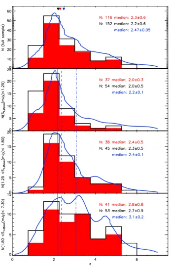
In Fig. 6 (top panel) we show the redshift distribution for our SMG sample. To investigate possible contamination of the red-shift distribution due to inclusion of uncertain redred-shifts, we show histograms of a strict sample, including only sources with spec-troscopic or unambiguous photometric redshifts (including both our own photometric redshifts and those from Marchesi et al. 2016), as well as an extended sample which includes all sources with redshift determinations or lower limits. The nine sources with lower limits are included in the histogram bin containing their limit. The strict sample consists of 116 sources and has a median redshift ˜z=2.3±0.6 (this uncertainty range corresponds to the median absolute deviation). The extended sample consists of 152 sources with a median of ˜z=2.2±0.6. The complementary set of 36 sources which are in the extended sample but excluded from the strict sample does appear to preferentially skew towards low redshifts. This is almost entirely due to our including those sources with redshift lower limits. When we exclude those nine sources with only redshift lower limits, a Kolmogorov-Smirnov (KS) test comparing the strict sample to the 27 sources in the complementary sample finds an associated probability of 0.32, providing no evidence that the samples are drawn from a di ffer-ent underlying population. In the same panel we also plot the redshift density likelihood function of the extended sample. This distribution is the cumulative addition of each source’s individ-ual redshift likelihood, constructed as in Miettinen et al. (2015a). Sources with spectroscopic redshifts are included as Dirac delta functions centered at zspec. Photometric and synthetic redshifts are included using their underlying likelihoods, and radio-mm and FIR-based redshifts are included as Gaussians with stan-dard deviations according to their associated redshift errors (as in the construction of the synthetic redshifts – see Sect. 4.5). The advantage of this estimation of the redshift distribution is that less certain redshift determinations affect the overall redshift dis-tribution less, and redshifts with significantly asymmetric posi-tive and negaposi-tive error bars can be appropriately accounted for. Sources with only lower limits are each included as a uniform likelihood extending from their lower limits to z=7 which avoids the problem of inappropriately reducing the overall redshift dis-tribution (seen in the slight difference between the median val-ues of the strict and extended histogram samples). We note that regardless of whether this small number of lower limits is in-cluded, our median redshift remains unchanged to two signif-icant figures. Redshifts are then randomly sampled from each of the 152 redshift likelihood functions and the sample median is determined in each of 1000 Monte-Carlo trials. The median value across all the Monte-Carlo runs is then reported as the redshift density likelihood function median, and the uncertainty corresponds to the range which encompasses 68% of the Monte-Carlo runs (i.e., 680 sample medians). Since this distribution properly takes into account the significant and asymmetric un-certainty in many of our redshifts, we take this to be the most accurate description of the sample redshift distribution. The me-dian of this distribution is ˜z=2.48±0.05.
With our large sample size, we are able to subdivide our sam-ple and directly examine how the redshift distribution is affected by the underlying flux density limit. In the bottom three panels of Fig. 6 we divide our sample roughly in thirds by flux density, showing the redshift distribution of sources with S1.25mm<1.25
Fig. 5: A comparison of the various redshift methods used in this work. For the top plot, photometric vs. spectroscopic, we have highlighted in red sources AzTEC/C61 and C8a which have am-biguous photometric redshifts. Source C61also has a synthetic redshift, which we have plotted as an open red circle. The large negative error bar for the photometric redshift of AzTECC61 has been suppressed for clarity. In the bottom plot, FIR vs. spectro-scopic, we have noted AzTEC/C113 and AzTEC/C45 which, de-spite meeting our criteria for being part of the training set, proved to be a significant outliers and were therefore ultimately ignored in our z vs. λpeakfit. The dashed line in each panel indicates a 1:1 redshift match.
Fig. 6: (Top panel:) Redshift distribution of our full SMG sam-ple. The filled red histogram includes only the 116 sources with spectroscopic or unambiguous photometric redshifts, our strict sample. The solid black line represents our extended sample, which additionally includes sources with radio-mm redshifts, FIR dust peak SEDs, less certain photometric redshifts, and sources which only have redshift lower limits. The smoothed blue line gives the redshift density likelihood function of the ex-tended sample. Median values are noted in the figure and plot-ted as red, black, and blue colored triangles for the strict sample histogram, extended sample histogram, and the extended sam-ple redshift density distribution (note that the strict and extended sample histogram medians are nearly coincident). (Bottom three panels:) The redshift distributions of our samples subdivided by their ALMA 1.25 mm flux density. Sources with flux densities Sν<1.25 mJy are shown in the second panel, 1.25 mJy ≤Sν≤1.8 mJy in the third, and Sν>1.8 mJy in the bottom panel. Our strict sample histogram, extended sample histogram, and redshift den-sity likelihood function are plotted as in the top panel. Three blue vertical lines spanning all three panels show the redshift density distribution median redshifts for the various subsamples. Solid, dashed, and dot-dashed lines correspond to the faintest to bright-est flux density divisions respectively.
mJy, 1.25 mJy <S1.25mm<1.8 mJy, and S1.25mm>1.8 mJy. The three flux density selections respectively include 37, 38, and 41 sources from our strict sample, and 54, 45, and 53 sources from our extended sample. The redshift density medians clearly in-crease with flux density, from ˜z=2.2±0.1 in the faintest sam-ple to ˜z=3.1±0.2 in the brightest sample, with strict and ex-tended samples presenting median values almost identical to each other. A KS test comparing the brightest and faintest ex-tended (strict) samples reveals an associated probability of 1.4e-3 (2.1.4e-3e-4) strongly indicating that the underlying redshift distri-butions in the brightest and faintest subsamples are different. 4.7. Multi-component SMGs
Several of our AzTEC/ ASTE sources are resolved into multiple components by ALMA. Given that a certain fraction of single-dish detected SMGs are expected to be composed of multiple systems in chance alignment, it is reasonable to ask how many of our multi-component sources are due to chance alignment and how many may be physically related (Wang et al. 2011; Hay-ward et al. 2013a). Here we discuss potential physical associ-ations based only on the source redshifts. For a discussion of the flux distribution among sources with multiple components see M. Aravena et al. (in prep), and for a comparison of our sample with clustering and evolutionary models see C. Jiang et al. (in prep). A total of 28 fields in our observations revealed two components within the area of the AzTEC primary beam. Among those resolved into two components, we consider nine pairs to be likely physical associations. The redshifts of the com-ponents in these paired systems are consistent with being iden-tical, and the individual redshift uncertainties are less than ±1. These systems include AzTEC/C 13, 22, 24, 28, 43, 48, 80, and 101. We also consider AzTEC/C 6 to be a likely physical as-sociation. Although the components C6a and C6b are separated by∆z=0.023, just slightly larger than the threshold Hayward et al. (2013a) suggest for differentiating between physical associa-tions and chance alignment, the system consists of at least five submm-bright sources (Bussmann et al. 2015) and is also located within an X-ray emitting cluster with 17 spectroscopically con-firmed member galaxies (Casey et al. 2015; Wang et al. 2016). The median separation of the pair components in all of our likely associations is 600. 5 (53 kpc at our median redshift, ˜z=2.47) with an interquartile range of 400. 9 to 1100. 3. The AzTEC/C6 and C22 systems, in particular, are likely to contain physically associ-ated components, as they each have spectroscopically confirmed components with similar redshifts. In the case of C22, the two components also appear to be connected by a radio-emitting bridge, which supports a scenario where the sources are gravita-tionally interacting (Miettinen et al. 2015b; Fig. 2 therein (their source AzTEC11); and Miettinen et al. 2017a).
An additional ten pairs are possible physical associations. Although their component redshifts are less well determined with uncertainties greater than ±1, they are within 1σ of one another. Their median component separation is 1300. 1 (106 kpc) with an interquartile range of 600. 5 to 1900. 2. Nine source pairs have larger redshift offsets, showing no signs of physical association (∆z>1σ). Their median component separation is 1200. 4 (100 kpc) with an interquartile range of 800. 0 to 1700. 0.
An additional five fields revealed three components. Three of these systems show tentative evidence that they may be phys-ically associated. The AzTEC/C9 triplet consists of two sources with spectroscopic redshifts of 2.922 and 2.884, and a third source with zphot = 2.68+0.24−0.51. Each of the components lies within 13” (101 kpc at z=2.9) of its closest neighbor. Although
these redshifts differ by more than is typical for physical as-sociations, the system lies within a BzK galaxy over-density. AzTEC/C90 includes three components within 13” (106 kpc at z=2.4) of one another and with photometric redshifts between 2.1 and 2.8. The AzTEC/C55 system includes one component with only a redshift lower limit, and two components with pho-tometric redshifts consistent with being identical. The compo-nents of this system are separated by up to 1700. 2 (141 kpc at z=2.55). The final triplet systems show no evidence of physi-cal association. AzTEC/C10 includes components separated by up to 1700. 4 (141 kpc at our median redshift, ˜z=2.47). Two com-ponents have effective lower limits from their radio-mm spec-tral indices (z3−240GHz = 3.40+3.60−0.59and z3−240GHz = 3.37+3.63−0.52 for C10a and C10c, respectively) and C10b has a redshift zsynth = 2.90+0.30−0.90, providing no useful evidence to evaluate their phys-ical association. AzTEC/C3 includes components separated by up to 20” (163 kpc). One component has only a redshift lower limit, one component, C3a, has a tentative zspec= 1.125 (as dis-cussed in Sect. 4.1), and one component has a radio-mm redshift, z3−240GHz = 2.03+1.19−0.31, which suggests that the components are a chance alignment.
5. Discussion
There is considerable discussion surrounding the differences in reported SMG redshift distributions and their associated selec-tion biases. Several studies of SMG redshifts suggest a positive correlation between flux density and median redshift (Ivison et al. 2002, Pope et al. 2005, Younger et al. 2007, Biggs et al. 2011, Smolˇci´c et al. 2012b), as well as a correlation between longer, mm-wavelength-based selections and higher redshifts (Blain et al. 2002, Zavala et al. 2014, Casey et al. 2013), while other works have not borne out this trend (Simpson et al. 2014, Miettinen et al. 2015a).
In Fig. 7 we compare the redshift distribution of our extended sample to previous SMG survey results. The sources represented in our redshift distribution are subject to two selection criteria: they were initially selected at or above a deboosted flux limit of 3.5 mJy at 1.1 mm on the ASTE instrument, and later detected by ALMA at 1.25 mm reaching a 5σ sensitivity of 750 µJy beam−1. While the initial 1.1 mm selection is a more restrictive flux limit, several sources are resolved as multiples by ALMA, indicating that the the achieved ALMA sensitivity also effects our sample selection.
Chapman et al. (2005) includes 76 SMGs selected from 850 µm SCUBA surveys which were identified with VLA radio counterparts and spectroscopically observed with Keck I to de-termine redshifts. Their SCUBA sample reaches a characteristic flux limit of 3 mJy, equivalent to 1 mJy at our selection wave-length of 1.25 mm. The radio observations reach a flux limit of 30 µJy. It is expected that the submm limit is most restrictive for SMGs at low redshifts, while the radio limit is most restric-tive at high redshift. Directly comparing our sample with theirs is complicated by the redshift desert at z∼1.5 for which few op-tical spectroscopic identifications were accessible, resulting in significant incompleteness in their sample over this range. After correcting for this incompleteness their calculated median red-shift is ˜z=2.2. We have attempted to compensate for the redshift desert in the histogram representation of their redshift distribu-tion in Fig. 7 in the same spirit as Smolˇci´c et al. (2012b). In ad-dition to the original Chapman et al. (2005) sample we augment the redshift distribution with 19 SMGs deliberately targeted in the redshift desert by Banerji et al. (2011), weighting the samples
by their survey area (721 arcmin2for Chapman et al. (2005) and 556 arcmin2for Banerji et al. (2011)) (Chapman, priv. comm.).
The sample from Simpson et al. (2014) is from an ALMA 870 µm follow up of the 870 µm LABOCA ALESS catalog (Hodge et al. 2013, Karim et al. 2013). Sources were identified with multiwavelength counterparts at wavelengths spanning UV through radio. Seventy-seven SMGs (ten with spectroscopic and 67 with photometric redshifts) were used to construct their red-shift distribution, resulting in a median redred-shift of ˜z=2.3±0.1. The Simpson et al. (2014) redshift distribution is similar to ours. With a KS probability of 0.87, we have no evidence to indicate the two samples are drawn from different underlying popula-tions. Much like our sample, the sources in the final redshift dis-tribution of Simpson et al. (2014) underwent two selection crite-ria, S870µm>4.4 mJy with LABOCA and a much fainter flux den-sity cut with ALMA. Their ALMA selection required S/N>3.5 and RMS<0.6 mJy beam−1 suggesting a characteristic source flux density limit ∼2.1 mJy at 870 µm. Assuming dust emission at z∼2.3 and β=1.5, the corresponding flux density at 1.25 mm is a factor of 2.8 lower, implying a limit of 740 µJy, very close to the characteristic flux limit for our ALMA sources. Indeed, the overall flux distributions of our sample and Simpson et al. (2014) shown in Fig. 8 are very similar, especially at the faint end. This suggests that survey flux limits are very important in explaining redshift distributions. Danielson et al. (2017) further investigated an ALESS sample by undertaking a spectroscopic redshift survey using optical and infrared spectrographs on the VLT and Keck telescopes. Their final sample, consisting of 52 sources with spectroscopic redshifts and 37 sources with pho-tometric redshifts, overlaps considerably with the sample from Simpson et al (2014), but the flux distribution of their sample is skewed slightly higher (Fig. 8). They also find a slightly higher median redshift of ˜z=2.4±0.1, but, comparing to our redshift dis-tribution, still shows no evidence of being drawn from a different underlying population than ours (a KS probability of 0.23).
The sample from Strandet et al. (2016) is a complete flux density limited sample at S1.4mm>16 mJy from the SPT Deep Field; it consists of 39 sources with spectroscopic redshifts identified primarily through ALMA spectral scans. Ambiguous sources with uncertain line identifications were followed up with targeted observations using APEX instruments FLASH, SEPIA, and Z-spec. In 35 sources, multiple line detections provide an un-ambiguous redshift, while in the remaining four sources a single line is detected and supporting FIR observations provide a rough redshift range and a most-likely line identification. The sources are expected to be strongly lensed due to their high flux density selection bias, so it is not surprising that their redshift distribu-tion has a significantly higher median redshift, ˜z=3.87. Strandet et al. (2016) attempt to account for the bias introduced by lens-ing by dividlens-ing their redshift distribution by the probability of lensing as a function of redshift, at an assumed lensing magnifi-cation of µ ∼10. This reduces their median redshift to ˜z=3.1 and effectively reduces their flux density cut to S1.4mm>1.6 mJy. For a modified black body with dust emissivity β=1.5 at z ∼3.1 the corresponding flux density at 1.25 mm is 2.23 mJy. For the 31 sources in our sample above this flux cut we find a very similar observed median redshift of ˜z=3.25.
The interferometric sample from Miettinen et al. (2015a) is based on a sample of 1.1 mm detected COSMOS SMGs ob-served with AzTEC on the James Clerk Maxwell Telescope (Scott et al. 2008). The fifteen brightest sources were then fol-lowed up with observations using the SMA at 890 µm (Younger et al. 2007, 2009) and the next fifteen with the Plateau de Bure Interferometer at 1.3 mm. Their selection at 1.1 mm, flux limited
to S1.1mm≥3.3 mJy, is very similar to ours, although their obser-vations at 1.3 mm are less sensitive, reaching an average RMS of 0.2 mJy and establishing a source flux density cut at 1.3 mm of ∼0.9 mJy. The redshift distribution of the 1.1 mm selected JCMT/AzTEC SMGs shown in Fig. 7 was revised from Mietti-nen et al. (2015a, 2017a). Twelve of these JCMT/AzTEC SMGs (AzTEC 1, 2, 4, 5, 6, 8, 9, 11-N, 11-S, 12, 15, and 24b) are com-mon with the present ALMA sample. The photometric redshifts from Miettinen et al. (2015a, 2017a, and references therein) were derived using a similar HyperZ analysis with SMG templates as in the present work. One exception is AzTEC 17a, for which Miettinen et al. (2017a) adopted a photo-z of 2.96+0.06−0.06from the COSMOS2015 catalog (Laigle et al. 2016) instead of the lower spec-z of 0.834 used earlier by Miettinen et al. (2015a). Also, the lower redshift limits for some of the JCMT/AzTEC SMGs were derived using the same Carilli-Yun redshift indicator (Carilli & Yun 1999, 2000) as employed in the present study. As described by Miettinen et al. (2017a), the sources AzTEC 24a and 24c were not detected in our ALMA 1.3 mm imaging of AzTEC 24 (=AzTEC/C48 field), and are very likely to be spurious. Hence, these sources were omitted from the redshift distribution plotted in Fig. 7. The final sample size is 37, out of which 25 sources are different from the present ALMA sample. Using the same survival analysis as in Miettinen et al. (2015a) to take the lower zlimits (right-censored data) into account, we derived the mean and median redshifts of hzi= 3.29 ± 0.22 and ˜z = 3.10 ± 0.28 for the revised redshift distribution of the JCMT/AzTEC SMGs. The quoted uncertainties represent the standard errors of the mean and median. If we cut our sample at a flux density of 0.9 mJy we find a redshift density median of ˜z=2.48. While this is lower than the JCMT/AzTEC SMGs, we are unable to determine if the difference is meaningful due to the small sample of sources that are not in common.
Previous works have attempted to model and predict ob-served redshift distributions based on underlying population dis-tributions and models of galaxy evolution and formation (e.g., Baugh et al. 2005; Lacey et al. 2016; Cowley et al. 2015; Bether-min et al. 2012, 2015). In particular, BétherBether-min et al. (2015) used their updated phenomenological models of main sequence and starburst galaxy evolution to model SMG number counts and redshift distributions. Their models characterize predicted red-shift distributions as a function of flux density limits and selec-tion wavelength, and they generally show good agreement with SMG surveys and bear out the correlation between brighter and longer wavelength-selected samples lying at higher redshifts. In Fig. 9 we show the Béthermin et al. (2015) predicted median redshifts at 1.2 mm as a function of flux limit, along with the results from our sample and from Simpson et al. (2014). Above our characteristic flux limit of 750 µJy, we find a median from our redshift density distribution of 2.49±0.05, consistent with the prediction of ˜z=2.49 from Béthermin et al. (2015). We also consider cutting our sample at the brighter flux densities used in Fig. 6, S1.25mm>1.25 mJy and S1.25mm>1.8 mJy (note that here we are cutting the sample based on a flux density minimum rather than a minimum and maximum as used in Fig. 6). Our median redshifts rise with the increasing flux density limit to 2.7±0.1 and 3.1±0.2, reflecting the consistent rise over this range dicted by Béthermin et al. (2015) and nearly matching the pre-dicted median redshifts of 2.70 and 2.86, respectively. This is a striking confirmation that flux density and wavelength selec-tion are crucial determining factors in redshift distribuselec-tion. We have also included the redshift predictions from Hayward et al. (2013b) in Fig. 9. Their faint selection at 1.1 mm (S1.1mm>1.5 mJy) is consistent with our observations. At greater flux
densi-Fig. 7: Redshift distribution of our extended sample (solid black line) compared to previous SMG surveys (green filled his-tograms). From top to bottom: Chapman et al. (2005) (cor-rected for redshift desert using SMGs from Banerji et al. (2011)), Simpson et al. (2014) as well as the updated ALESS sam-ple from Danielson et al. (2017) (orange dashed histogram), JCMT/AzTEC SMGs (revised from Miettinen et al. (2015a, 2017a)), Strandet et al. (2016). Histograms have been normal-ized by their sample size such that each histogram contains equal area. Median values for each distribution are indicated by trian-gles above the distributions. (Here we use our observed median redshift ˜z=2.3 rather than the median calculated from the red-shift density likelihood function to compare directly to the other surveys’ observed medians.)
ties their prediction differs considerably from Béthermin et al. (2015), however we do not have a sufficient sample at these flux densities to test the respective models. The data from Simpson et al. (2014) follows a similar trend. Their median redshift is 2.31±0.06 for their sample above their characteristic flux limit of ∼2.1 mJy. Considering only the brightest 50% of sources in their sample (S870µm>4.4 mJy), the median redshift rises to 2.5±0.1. These redshift are nearly consistent with although slightly lower than the 850 µm predictions by Béthermin et al. (2015) of 2.5 and 2.7, respectively.
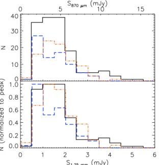
Fig. 8: (Top panel) Flux density distribution for our extended sample (solid black line), the Simpson et al. (2014) ALESS sam-ple (blue dashed line), and the Danielson et al. (2017) ALESS sample (orange dot dashed line). The top x-axis, noting S870µm for the ALESS samples, has been scaled from S1.25mmby a fac-tor of 2.8 corresponding to the ratio of continuum emission ob-served at 870 µm vs. 1.25 mm coming from a modified black-body with emissivity β=1.5 at z ∼2.4. (Bottom panel) Same as the top panel, but the samples have been normalized to their peaks to compare relative sample sizes.
6. Summary
Our ALMA observations provide one of the deepest mm se-lected SMG surveys with high spatial resolution, ∼1”. We de-tect a total of 152 sources within our primary beam at greater than 5σ significance, with an average RMS of 150 µJy beam−1. Although SMGs are typically difficult to cross-identify at other wavelengths, the high resolution of our survey combined with the broad multiwavelength coverage in COSMOS allows us to unambiguously identify counterparts across the UV-NIR, FIR, and radio spectral regimes. This unique data set permits us to compile the spectroscopic redshifts for 30 sources, as well as photometric redshifts for 113 sources through a variety of meth-ods including UV-NIR photometric fits, radio-mm spectral in-dices, and FIR dust SED fits. For the remaining nine sources, we determine lower redshift limits. While some redshift estima-tions have large uncertainty, (particularly those redshifts deter-mined through radio-mm spectral indices, FIR dust SED fitting, or ambiguous UV-NIR photometric fits), these do not appear to systematically affect our redshift distribution.
Our sample has a median redshift of ˜z=2.48±0.05, gener-ally consistent with previous SMG distributions. Simpson et al. (2014) and Chapman et al. (2005) both find very similar median redshifts. Although recent work by Strandet et al. (2016) finds a significantly higher median redshift of ˜z=3.87, this difference is well explained by their very bright flux limit, which largely restricts their sample to highly lensed sources. Deeper investiga-tion into subsets of our sample, split by flux density, bear out the trend toward higher redshifts with increasing flux density limits. In particular, our 1.25 mm data, restricted to various flux limits, show redshift distributions very consistent with the models of Béthermin et al. (2015).
Fig. 9: Green circles denote our survey results which include the extended sample above the characteristic flux limit of 750 µJy, and also cut at S1.25mm >1.25 mJy and S1.25mm >1.8 mJy. Cyan squares denote results from Simpson et al. (2014), including the sample above their characteristic flux limit of 2.1 mJy and also cut at S870µm > 4.4 mJy such that half their sample is included. Plotted results and error bars represent the medians calculated through our Monte-Carlo trials and the extent of 68% of the me-dian values. Meme-dian redshift as a function of survey flux den-sity limit is also shown. The green and cyan lines give model predictions based on Béthermin et al. 2015. Models from Hay-ward et al. (2013b), plotted as green (blue) crosses, give mean redshift estimates for 1.1 mm (850 µm) at flux density limits of S1.1mm >1.5 mJy and S1.1mm >4.0 mJy (S850µm >3.5 mJy and S850µm >9.0 mJy). Our observed redshift distribution rises with increasing flux density limits, consistent with both the models of Béthermin et al. (2015) and Hayward et al. (2013b).
The high resolution of our survey reveals several submm sources to be multi-component systems. A thorough investiga-tion of their physical associainvestiga-tions is beyond the scope of this paper, however, based on the redshifts of the components within our multiple systems, we have identified nine likely and 13 pos-sible physical associations of SMGs. An additional eleven sys-tems either have no evidence for physical association (compo-nents with unidentified redshifts), or evidence indicating chance alignment (widely discrepant component redshift estimates).
7. Acknowledgements
We thank the anonymous referee for insightful comments and advice. D. B. acknowledges partial support from ALMA-CONICYT FUND No. 31140010. and FONDECYT postdoc-torado project 3170974. M.A. acknowledges partial support from FONDECYT through grant 1140099. V. S., O. M. and I. D. acknowledge funding from the European Union’s Seventh Framework program under grant agreement 337595 (ERC Start-ing Grant, ‘CoSMass’). The work of O. M. was performed in part at the Aspen Center for Physics, which is supported by National Science Foundation grant PHY-1066293. The work of O. M. was partially supported by a grant from the Si-mons Foundation. A. K. acknowledges support by the Col-laborative Research Council 956, sub-project A1, funded by the Deutsche Forschungsgemeinschaft (DFG). C. M. C. thanks UT Austin’s college of natural science for support. D.R. ac-knowledges support from the National Science Foundation
der grant number AST-1614213 to Cornell University. C.J. ac-knowledges support from Shanghai Municipal Natural Science Foundation (grant 15ZR1446600) The Flatiron Institute is sup-ported by the Simons Foundation. This paper makes use of the following ALMA data: ADS/JAO.ALMA#2013.1.00118.S and 2011.0.00539.S. ALMA is a partnership of ESO (representing its member states), NSF (USA) and NINS (Japan), together with NRC (Canada), NSC and ASIAA (Taiwan), and KASI (Repub-lic of Korea), in cooperation with the Repub(Repub-lic of Chile. The Joint ALMA Observatory is operated by ESO, AUI/NRAO and NAOJ. This research has made use of data from HerMES project (http://hermes.sussex.ac.uk/). HerMES is a Herschel Key Pro-gramme utilizing Guaranteed Time from the SPIRE instrument team, ESAC scientists and a mission scientist. HerMES is de-scribed in (Oliver et al. 2012).