HAL Id: tel-00439669
https://tel.archives-ouvertes.fr/tel-00439669
Submitted on 8 Dec 2009
HAL is a multi-disciplinary open access
archive for the deposit and dissemination of
sci-entific research documents, whether they are
pub-lished or not. The documents may come from
teaching and research institutions in France or
abroad, or from public or private research centers.
L’archive ouverte pluridisciplinaire HAL, est
destinée au dépôt et à la diffusion de documents
scientifiques de niveau recherche, publiés ou non,
émanant des établissements d’enseignement et de
recherche français ou étrangers, des laboratoires
publics ou privés.
A study of the performance of a nulling interferometer
testbed preparatory to the Darwin mission
Pavel Gabor
To cite this version:
Pavel Gabor. A study of the performance of a nulling interferometer testbed preparatory to the Darwin
mission. Astrophysics [astro-ph]. Université Paris Sud - Paris XI, 2009. English. �tel-00439669�
´
ETUDE DES PERFORMANCES D’UN BANC
INTERF ´
EROM ´
ETRIQUE EN FRANGE NOIRE
DANS LE CADRE DE LA PR ´
EPARATION
DE LA MISSION DARWIN
Soutenue publiquement le 22 septembre 2009 devant le jury :
Jean-Pierre Bibring,
Pr´esident
Peter Lawson,
Rapporteur
Franc¸ois Reynaud,
Rapporteur
Jonathan Lunine,
Examinateur
Daniel Rouan,
Examinateur
Alain L´eger,
Directeur de th`ese
0.5 Organisation of the dissertation . . . ix
1 Astrobiology and Exoplanetology 1 1.1 Are we alone? . . . 1
1.1.1 What is life? . . . 1
1.1.2 Current scientific approaches. . . 4
1.2 Exoplanets. . . 5
1.2.1 Indirect detection . . . 6
1.2.2 Direct observation . . . 7
1.2.3 Step by step . . . 9
1.3 Formation-flying nulling interferometer . . . 9
1.3.1 Design overview . . . 10 1.3.2 Nulling ratio . . . 11 1.3.3 Stability. . . 13 2 Nulling Interferometry 15 2.1 Bracewell’s principle . . . 15 2.2 Performance parameters . . . 16
2.3 Achromatic Phase Shifters . . . 18
2.4 The Dispersive Prisms APS. . . 20
2.5 Wavefront filtering . . . 20
2.6 Stability . . . 22
ii CONTENTS
3 Description of S & N 27
3.1 Introduction . . . 28
3.1.1 The purpose of this Chapter . . . 28
3.1.2 General note . . . 28
3.1.3 Historical background . . . 29
3.2 General overview . . . 32
3.2.1 An outline . . . 32
3.2.2 General layout . . . 33
3.3 Purpose of the subsystems . . . 36
3.3.1 A point source observed by two apertures . . . 36
3.3.2 Three remarks on single-mode fibres. . . 36
3.3.3 Off-axis parabolic mirrors . . . 37
3.3.4 Symmetry. . . 38
3.3.5 Flux balancing . . . 40
3.3.6 Stability. . . 41
3.3.7 Optical path . . . 43
3.4 Sources . . . 44
3.4.1 Ceramic black body . . . 44
3.4.2 3.39 µm HeNe laser . . . 46
3.4.3 Supercontinuum laser source . . . 46
3.4.4 2.32 µm laser diode. . . 47
3.5 Modal filters. . . 48
3.5.1 Fluoride-Glass Single-Mode Fibres . . . 48
3.5.2 Fibre output aperturing . . . 48
3.6 Spectral filters . . . 48
3.7 Polarisers . . . 50
3.8 Detectors . . . 50
3.8.1 Array detector . . . 50
3.8.2 Single element detector. . . 50
3.9 Phase shifter prototypes. . . 53
3.9.1 Focus Crossing or Through Focus . . . 53
3.9.2 Field Reversal or Periscope. . . 53
3.9.3 Dispersive prisms. . . 54
3.10 Electronics & Software . . . 54
3.10.1 Lock-in amplifier . . . 55
3.10.2 Software . . . 56
3.11 S . . . 60
4.3.3 Cycle parameters . . . 70
4.4 Results. . . 72
4.4.1 K band . . . 72
4.4.2 Laser light . . . 75
4.5 Comparison with some other experiments . . . 77
4.6 Discussion. . . 77
5 S results update 81 5.1 Preliminaries . . . 82
5.1.1 Thermal and mechanical instability . . . 82
5.1.2 Detector calibration. . . 82
5.1.3 Transmission . . . 82
5.2 Techniques . . . 83
5.2.1 Zero optical path difference and the CaF2Prisms . . . 83
5.2.2 Fringe dispersion . . . 83
5.2.3 Fourier transform . . . 84
5.2.4 Direct nulling measurements . . . 84
5.2.5 Experimental protocol . . . 84
5.3 Nulling levels reached with S . . . 85
5.3.1 The 2000 K black body. . . 86
5.3.2 First effective stabilisation . . . 86
5.3.3 3.39 µm HeNe laser and polarisers . . . 86
5.3.4 S II: Improved mechanics and alignment . . . 89
5.3.5 Supercontinuum source. . . 89
5.3.6 Focus crossing APS . . . 89
5.3.7 Narrow band centred at 2.3 µm. . . 90
5.3.8 Fibre curvature . . . 90
5.3.9 L band . . . 90
iv CONTENTS
6 Error budget 93
6.1 Tests and models . . . 93
6.1.1 Detector nonlinearity . . . 93
6.1.2 Beam path . . . 94
6.1.3 Polarisation . . . 94
6.1.4 Chromatic shear and other dispersive effects. . . 96
6.1.5 CaF2Prisms: multiple working points . . . 98
6.1.6 Coatings . . . 99 6.1.7 Inhomogeneities . . . 99 6.1.8 Spectral mismatch . . . 101 6.1.9 Wavefront quality. . . 101 6.2 Testing on N. . . 102 6.3 Error budget . . . 102 6.4 Summary . . . 104
7 Conclusions and perspectives 105 7.1 What was to be done . . . 105
7.2 What was done . . . 106
7.2.1 My contribution . . . 106
7.3 Perspectives . . . 107
7.3.1 N . . . 107
7.3.2 Polarisation . . . 107
7.3.3 Tests of achromatic phase shifters . . . 107
7.3.4 Flux-balance stabilisation . . . 108
7.3.5 Experiments around 10 µm. . . 108
7.4 Towards a flagship space mission . . . 108
7.5 Summary . . . 109
Appendices 111 A Cosmic Pluralism 113 A.1 Millennia of speculation . . . 113
A.2 Links and implications . . . 113
A.3 Historical notes . . . 114
A.3.1 Three forms of cosmic pluralism . . . 114
A.4 Ideology and historiography . . . 116
A.4.1 “Pre-Socratic light”. . . 116
A.4.2 “Medieval darkness” . . . 117
A.4.3 Nicolas of Cusa . . . 118
a style where I try to explain things in simple terms. In order to do that I was often led to a deeper understanding of the subject matter.
Most of all, I am grateful for this opportunity to take a step back, and look at my work in a broader context, with a deeper understanding, and a better grasp of the network of details which is an experiment’s fibre of being.
0.1
Teamwork
Ptolemy (Almagest IX, 2) mentions that Hipparchus refrained from formulating a definitive theory of plane-tary motion, providing a legacy of observations to future generations, whom Hipparchus invited to continue collecting data to the best of their ability. Ever since Hipparchus realised that one lifetime’s worth of as-tronomical observations cannot provide empirical evidence of sufficient scope to decide certain scientific issues, astronomy has been the first discipline to become aware of itself as a collective effort (ˇSpelda 2006, , p. 243) spanning generations. In recent decades, teamwork has become the rule in astronomy, especially when it comes to the construction of instruments, data acquisition and reduction.
0.2
Initiation
How does a humble adept become a part of this wonderful adventure? First, there is some schoolwork in order to acquire sufficient knowledge and a some skills. But I now view all of my years of study as mere preparation for the real challenge, the rite of passage called “PhD”. Then he enters a cavern where the initiation takes place, labouring there not for nine days like the Greater Eleusinian Mysteries, but for three years!
My previous experience allowed me to realise the importance of being with good people. I am very grateful to Michael Heller, George Coyne, Pierre-No¨el Mayaud, Pierre L´ena, and Daniel Rouan who en-couraged me and helped me choose the door on which to knock.
viii 0.3. WORK IN A TEAM: MY ACKNOWLEDGMENTS
0.3
Work in a team: my acknowledgments
Then the door opened, allowing me to enter and participate in the Mysteries. I stepped over the thresh-old with trepidation. What frightful challenges would I have to face? Would I have to face them alone, struggling to overcome them surrounded by indifference or even hostility at the Temple called “Institut d’Astrophysique Spatiale”?
I am at a loss how to express how fortunate I feel to have found such a wonderful group of people there. Let me merely list the names (in the order in which I met them): Alain L´eger, the paradigm of a physicist; Marc Ollivier, the brilliant experimentalist and nulling pioneer; Frank Brachet, the builder of S; Bruno Chazelas, the open-source wizard; Sophie Jacquinod, also known as Sophie Bond; Michel Decaudin, the star optician; Alain Lab`eque, the intrepid inceptor of S; Jo¨el Charlet, the elusive elec-trician; Claude Valette, the cryogenic cameraman; Pascal Bord´e, the moving spirit of the press review; Philippe Duret, the irreplaceable and imaginative Chagall of Shadoks; Vaitua Leroi, the friendly Martian; Peter Schuller, the fringe forebear/foreman; Benjamin Samuel, the Periodographic Nimrod; Thomas Lau-rent, who accompanied us on our obscure path but for a short while; and finally, Olivier Demangeon, my courageous successor.
I am truly sorry that I cannot list everybody, and I know this is not right. Let me at least mention two more categories of people. John S. Bell in one of his papers on quantum systems remarks that quantum measurements are interactions between microscopic sytems and macroscopic systems, the latter being dif-ficult to delimit, and he asks whether the institute’s administrative staff should also be counted as a part of the measuring apparatus. After my experience at the Institut d’Astrophysique Spatiale I have become convinced that all the “support” staff was very much a part of the team, and contributed significantly to our work.
Last but not least I would like to mention our colleagues from Nice, Cannes, Heidelberg, Li`ege, Delft, Grenoble, Pasadena — Yves Rabbia, Jean Gay, Marc Barillot, Ralf Launhardt, Olivier Absil, Pierre Kern, Peter R. Lawson, Bob Peters, Stefan Martin, Andrew Booth, Rob Gappinger, and all the nulling interfer-ometrist around the world. May the light of nulling grow ever fainter!
Working as a team without reaching the expected performance parameters and results, we had to master our frustration, maintain good morale, perseverance and creativity. Regardless of how the optical experi-ment went, the sociological and psychological one was an extraordinary success.
In most of the text, I shall not even try to describe my contribution. More often than not the collective “we” does not stand for the author but for the team. An account of my personal efforts will be given in the last Chapter (7.2.1).
0.4
Goals and objectives
In distinguishing goals and objectives I am following a usage where “goals” are general teleological per-spectives, whereas “objectives” are concrete performance parameters to be reached by a given date. The objectives were primarily imposed by outside commitments (an ESA contract). During the period of my graduate studies they evolved quite considerably. Just as an example, let me mention that at first we worked towards testing three achromatic phase shifter prototypes, by the end of 2008 this goal was practically no longer an objective (although it remained a goal – the difference being that there is no deadline set for the tests). I shall therefore not present our work against the background of these shifting objectives, but rather of the goals which remained unchanged throughout.
In this sense, the goals of this work are twofold. First, there are the science goals, namely, advancement of nulling interferometry in view of a future interferometric space mission capable of detecting biomarkers in spectral studies of Earth-like extrasolar planets. Second, there are pedagogical goals of the hands-on training in intrumental development. Although the pedagogical goals are, ultimately, the main purpose of post-graduate study, the dissertation is not the place to discuss them in any detail. Let me just say that I am very grateful that I worked in a small group where we had to develop many things from scratch and we
0.5
Organisation of the dissertation
A French r´esum´e is added at the very end of the volume, hopefully making it easier to find without a lot of page-turning.
The first two Chapters introduce the subject. The first (Chap.1) gives a very brief overview of the issue of cosmic pluralism in the context of current scientific research. The second (Chap.2) describes the principles of nulling interferometry. Chapter3is a description of the testbeds at Institut d’Astrophysique
Spatiale, Orsay, called S and N. Chapter4describes a stabilisation technique which we developed and used during our work on the testbeds. It closely follows the papersGabor et al.(2008a,b). Chapter 5 is a report on the results obtained with S II, closely following the articleGabor et al. (2008c). (Readers who are familiar with these papers can skip Chapters4,5, and go directly to Chapter6 which is a presentation of our work aiming to achieve a better understanding of the broadband null-depth limitation, performed on S II. Chapter7describes what was to be done, what was done, my personal contribution, what is to be done, i.e., future work to be carried out on the N testbed, and some conclusions, including those regarding the broader context of spaceborne nulling interferometry.
1.1.2 Current scientific approaches. . . 4
1.2 Exoplanets . . . . 5
1.2.1 Indirect detection . . . 6
1.2.2 Direct observation . . . 7
1.2.3 Step by step. . . 9
1.3 Formation-flying nulling interferometer . . . . 9
1.3.1 Design overview . . . 10
1.3.2 Nulling ratio . . . 11
1.3.3 Stability. . . 13
1.1
Are we alone?
The question of cosmic pluralism has a long and complicated history, linked to its many interdisciplinary overlaps. AppendixAcontains a study on the subject1. Speculation was the only possible approach for generations. The scientific community is currently developing observational techniques designed to bring the first quantitative answers. This dissertation is an account of a small part of these efforts.
1.1.1
What is life?
The speculation on humanity’s uniqueness or mediocrity is doubtless fascinating in its own right but in order to explore all the possible scientific approaches we shall have to broaden the horizon of our investigation to include not only intelligent extraterrestrials but life in the Universe in general. Hence the question: “What is life?”
The discussion is ongoing. As the historian of science, James Strick, puts it:
What is life? Is it the assemblage of the operations of nutrition, growth, and destruction, as Aristotle thought? Or is it organization in action, as French physician and biologist Franc¸ois-Xavier Bichat defined it? Or might it be the continuous adjustment of internal relations to 1Presented at the conference Darwin’s Impact on Science, Society, and Culture held in Braga (Portugal), 9-12 September 2009.
2 1.1. ARE WE ALONE?
external relations, as the British philosopher and sociologist Herbert Spencer believed? (Strick 2003)
Let us make it quite clear from the outset that we are not going to discuss the question of the nature of life. It is by and large still an open issue with a captivating history and an even more confused historiography than cosmic pluralism.
We shall limit ourselves to an utilitarian approach, providing a rough outline of what exactly is meant by the extraterrestrial life that contemporary science seeks. We shall completely forego certain important chapters from the history of scientific thought, such as the theory of vitalism, in order to concentrate on the current position of the problem, starting with the Fermi Paradox, introducing Drake’s Equation, and ending with a discussion of extremophiles, silicon-based life and spectroscopic biomarkers.
1.1.1.1 The Fermi Paradox
Stephen Webb presents the “canonical version” of the episode established byJones(1985):
Fermi was at Los Alamos in the summer of 1950. One day, he was chatting to Edward Teller and Herbert York as they walked over to Fuller Lodge for lunch. Their topic was the recent spate of flying saucer observations. Emil Konopinski joined them [... Then] there followed a serious discussion about whether flying saucers could exceed the speed of light. [...] The four of them sat down to lunch, and the discussion turned to more mundane topics. Then, in the middle of the conversation and out of the clear blue, Fermi asked: “Where is everybody?” His lunch partners Teller, York and Konopinski immediately understood that he was talking about extraterrestrial visitors. And since this was Fermi, perhaps they realised that it was a more troubling and profound question than it first appears. York recalls that Fermi made a series of rapid calculations and concluded that we should have been visited long ago and many times over. (Webb 2002, pp. 17-18)
A quantitative estimate of the number of space-worthy extraterrestrial civilisations in our own Galaxy, the Milky Way, led Enrico Fermi to the conclusion that there must be millions of them. Different authors after Fermi obtained different results, and it should be noted that Fermi’s estimate is one of the more optimistic ones. Indeed, it would appear that over the last six decades sentiments among researchers have varied widely, and that some even find that pessimism and optimism have been coming and going in waves, an optimistic period succeeding a pessimistic one over the decades.
The discovery of extrasolar planets has, understandably, brought about a wave of optimistic estimates which is largely still upon us. Let us note, however, that (Santos et al. 2003) seem to indicate that our own planetary system, the Solar system, is rather unique since it would appear that giant planets migrate towards their stars in the early stages of the system’s formation more often than not. The fact that Jupiter did not migrate through the habitable zone is very likely an important factor in the emergence of life on Earth. We shall not enter into the detail of this speculation: we believe more data are vitally needed in order to obtain a clearer picture of comparative planetology. Suffice it to say, that this study, as well as other convictions, led a number of researchers to adopt a more pessimistic view of cosmic pluralism in recent years. They would appear to be in a minority, nonetheless.
1.1.1.2 Drake’s Equation
Ever since the 1960’s, Fermi’s estimate of the number of extraterrestrial civilizations in our Galaxy with which we might come in contact has been facilitated by the factorisation known as the Drake equation (Drake 1961; Drake and Sobel 1992). It permits us to quantify the individual factors intervening in the estimate:
• fiis the fraction of the above that actually go on to develop intelligent life,
• fcis the fraction of the above that are willing and able to communicate,
• L is the expected lifetime of such a civilization.
In this form, the temporal limitations are included as the product R∗L, i.e., the rate of star formation
per unit of time multiplied by the lifetime of a civilisation. Another form of the equation is often used, determining the same temporal limitations taking the expression N∗L/T∗, where N∗is the number of stars in the Galaxy and T∗is a star’s lifetime. This alternative form can thus be written as:
n = N∗× fp× ne× fl× fi× fc× L
T∗ (1.2)
Contemporary empirical knowledge allows us to obtain estimates of some of these factors and of their uncertainties. Currently, the value of R∗ is estimated as 7 per year (one also often encounters the older estimate of R∗= 10 per year). Using the alternative approach, the value of N∗can be estimated as 1.6 1011,
whereas T∗can be taken as equal to
T∗= M∗
M⊙
!−2.5
1010years, (1.3)
i.e., for stars with M∗= 0.75M⊙we obtain
N∗ T∗ =
1.6 1011
(M∗/M⊙)−2.51010 per year = 8 per year, (1.4)
roughly the same number as our estimate for R∗.
The study of the extrasolar planets in the next two decades is likely to lead to good estimates for the values of fpand ne. The issue at hand is a better understanding of mechanisms behind the formation and
evolution of planetary systems. The factor neis often understood as the number of planets per star which
are in the so called “habitable zone”, i.e. at such a distance from the star where liquid water can be found on their surface. Naturally, this is already a statement of a position regarding the physical and chemical conditions for life.
So far, we have little useful observational evidence for an assessment of the factor fl. Indeed,
consider-ing how controversial and problematic a definition of “life” is, it is rather doubtful that a reasonable answer will be forthcoming in the next one or two generations.
However, if we restrict our notion of “life” somewhat, and make some presumptions about its biochem-istry, we may be able to find a value of the factor flthrough spectroscopy of exoplanetary atmospheres.
4 1.1. ARE WE ALONE?
1.1.1.3 Identifiable life
There are several assumptions that we can safely make about the chemistry of the life we want to search for. There are two aspects to this restriction. One has to do with feasibility and practicality: There may be other sorts of life but they would be even harder to identify. The other has more to do with our scientific understanding of the processes involved: It seems that it is easier for complex structures to form under certain conditions rather than under other conditions.
Two or three such assumptions stand out as an intersection of consensus among most researchers. Thus, we expect this “identifiable life” to
• be based on the chemistry of the element carbon simply because the alternatives (e.g., silicon) appear considerably less promising;
• have biomembranes defining the internal volume of the lifeform as opposed to its environment; • use liquid water: this is mostly understood as “life in a liquid-water solution” but it could just mean
that water is likely to play a rˆole in the metabolic processes of all lifeforms.
Obviously, this still leaves a very broad space to explore. An interesting approach is based on the idea of hypothetically detecting terrestrial life from space. Studies (e.g.,Kaltenegger et al. 2007) were conducted to see whether the presence of a biosphere on Earth could have been detected by remote sensing over our planet’s history. Spectroscopic methods may be able to detect the presence and mutual proportion of various chemicals in the planetary atmospheres.
1.1.1.4 Spectroscopic biomarkers
Supposing that sought-after extra-solar life is somewhat akin to the terrestrial biosphere, we may expect to observe its spectroscopically blatant impact on extra-solar planetary atmospheres. The possibility that O2and O3are ambiguous identifications of Earth-like biology, but rather a result of abiotic processes, has
been considered in detail (L´eger et al. 1999;Selsis et al. 2002). Various production processes have been evaluated, e.g., abiotic photodissociation of CO2and H2O followed by the preferential escape of hydrogen
from the atmosphere, cometary bombardment introducing O2 and O3 sputtered from H2O by energetic
particles. The conclusion is that a simultaneous detection of significant amounts of H2O and O3 in the
atmosphere of a planet in the habitable zone presently stands as a criterion for large-scale photosynthetic activity on the planet. Future space missions like Darwin and TPF-I thus focus on the region between 6 µm to 20 µm, containing the CO2, H2O, and O3spectral features of the atmosphere.
Spectroscopic search for biological markers in exo-planets is therefore a goal to be achieved. The issue at hand is, “How?”
1.1.2
Current scientific approaches
We have introduced Drake’s equation and we mentioned the issue of identifying the presence of a biosphere on an exoplanet. Let us now take a step back and look at the panorama of current scientific approaches to the question: “Are we alone?”
1.1.2.1 SETI
Drake’s equation was inspired by the search for extraterrestrial civilisations rather than extraterrestrial life as such. We saw that some of the factors in the equation can be estimated by astrophysical observations. There is another avenue that is worth exploring, however. If there are extraterrestrial civilisations out there, they might produce artificial radiation in the domain of radio waves. In other words, they might be producing identifiable signals. And it would suffice to listen attentively in order to receive them. This programme is known as SETI, the Search for ExtraTerrestrial Intelligence.
Titan. The largest of Saturn’s moons, Titan, was the destination of the Huygens-Cassini space mission. The instruments reached Saturn’s system in June 2004. The Huygens probe descended into Titan’s atmo-sphere discovering a new and intriguing world where liquid methane plays a rˆole analogous to water on Earth: there are vast lakes of methane, and methane rainfall. Cassini remains in orbit around Saturn updat-ing our knowledge of the surface of Titan at every flyby. The most interestupdat-ing point regardupdat-ing Titan is this: If we find life there, based on methane as solvent, it becomes clear that life emerged independently twice in the Solar System. If it happened twice in one planetary system, it is very likely that life is ubiquitous in the Universe.
Enceladus. The Cassini mission discovered evidence that Enceladus, a natural satellite of Saturn, resem-bles Europa in having an ocean of liquid water under a crust of ice. Space mission proposals to study the Saturn system were submitted to the US and European space agencies (Titan Saturn System Mission, TSSM; Titan and Enceladus Mission, TandEM), and although a joint mission to the Jupiter system (EJSM) was selected in February 2009, the mission to Saturn’s satellites will continue to be studied.
1.1.2.3 Exoplanetology
One of the most dynamic fields of astrophysical inquiry is exoplanet research. Its goals are • a survey of planetary systems and a classification of their types,
• a census of exoplanets and their typology, morphology and geophysics, • a better understanding of planet formation and the underlying mechanisms, and • a study of the properties of exoplanetary atmospheres.
This list does not pretend to be exhaustive. Its purpose is to show that exoplanetology searches for answers that are of utmost pertinence to astrobiology.
1.2
Exoplanets
The direct observation of an exoplanet, in the sense of identifying and studying the photons emitted by an exoplanet, is very challenging. There are three major obstacles to be surmounted:
1. angular resolution: levels better than 0.1 arcsec are needed because there always is a very bright object at a very small angular distance, viz., the parent star around which the exoplanet revolves;
6 1.2. EXOPLANETS
2. the contrast in brightness between the exoplanet and its star is such that even the starlight contained in the comparatively very dim outer diffraction pattern is still brighter than the planet; and
3. zodiacal and exozodiacal light, i.e., the environment of the Earth and of the observed exoplanet (as well as the intervening cosmic medium) contains sources of diffuse thermal emissions (gas and dust) at the same wavelength as those of the exoplanet.
1.2.1
Indirect detection
These challenges mean that direct observation of exoplanets cannot be performed so far. The information we have gained comes from indirect detection methods.
There are two types of effects of the exoplanet on the observation of its parent star:
1. motion: the orbital movement of the exoplanet influences the position of the observed star’s photo-centre;
2. photometry: the presence of the exoplanet may influence the brightness of the observed star. The orbital motion of an exoplanet is coupled with an orbital motion of the star around a common centre of mass. Each of the bodies revolves on an elliptical path with the centre of mass in one of its foci. The semimajor axis a∗of the star’s orbit can be expressed in terms of the semimajor axis of the exoplanet’s orbit
apand of the masses of the star and of the exoplanet, m∗and mp, respectively, as follows:
a∗= mp
m∗+ mp
ap. (1.5)
This means that the star is in motion which is due to the orbital movement of the exoplanet. The star’s velocity vector can be decomposed into the component along the line of sight from the Earth and into the two components in the plane tangent to the celestial sphere.
There are five methods based on these phenomena:
1. Astrometry: which observes the motion of the star on the celestial sphere. It provides an unambigu-ous measure of the planet’s mass and orbital parameters.
2. Radial velocimetry: which measures the radial component of the star’s velocity vector using spectro-scopic methods. Using this technique, the planet’s mass can be determined only indirectly as m sin i where i is the inclination of the planet’s orbit with respect to the line of sight.
3. Pulsar timing: which also measures the radial component of the star’s velocity vector, but applied to pulsars, this quantity can be deduced from the precise timing of the their pulses.
4. Transits: If the exoplanet passes in the line of sight between its parent star and the Earth, the star’s light appears to decrease somewhat during the exoplanet’s transit in front of the star’s disc. This technique allows the planet’s size to be estimated. In conjunction with radial velocimetry, it provides a measure of the exoplanet’s density (the m sin i ambiguity is minimised by the fact that orbital planes of transiting exoplanets must be approximately aligned with the line of sight).
5. Gravitational microlensing: When a massive object lies between the observer and the observed object, the image of the latter can be deformed by the gravity of the lens, i.e., the intervening object. In a simple case, the lens amplifies the light of a faint star. If there is a favourably positioned exoplanet orbiting the star, then the lightcurve of the microlensing event contains a secondary peak due to the exoplanet. No follow-up observations of the objects detected by this technique are likely, and therefore the primary contribution of gravitational microlensing to exoplanetology is in statistical estimates of exoplanet populations.
D
where λ is the wavelength. This means that working in the visible domain a telescope smaller (typically a few metres) than in the infrared suffices to overcome diffraction. In the infrared domain, a single telescope will not be practical.
At the same time it must be noted that the star-planet contrast is wavelength-dependent. Fig.1.1shows that the spectrum of the Earth contains three elements:
1. The reflected sunlight with its peak in the visible domain; λmax=
b Teff
=2898 µm K
5778 K ≈ 0.5 µm; (1.7)
2. Earth’s thermal emission with the peak at λmax=
2898 µm K
300 K ≈ 10 µm; (1.8)
3. absorption features of various molecules in the Earth’s atmosphere.
The spectral region highlighted in Fig.1.1offers two advantages over the visible:
• It features essential biomarkers,
• the star-planet contrast is the least unfavourable.
As was already said, a single telescope in the infrared spectral range, would need to have a very large aperture because of diffraction. The alternative is to employ interferometric techniques. This leads us to the disadvantages of the infrared:
• Multiple space telescopes are needed, and • they need to fly in formation.
Coronography. The approaches studied for exoplanet observation in the visible spectral range concen-trate on coronography. There are two basic concepts:
• A single spacecraft with a sophisticated optical payload, including a substantial primary mirror (Fig.1.2);
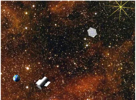
• A simple space telescope with another spacecraft at a distance of about 50 000 km whose rˆole would be to carry an occulting screen (Fig.1.3).
2Even though in some favourable cases the transit method can allow for such separation of the photons emitted by the planet itself
8 1.2. EXOPLANETS
Figure 1.1 - Sun-Earth contrast observed from 10 pc with the main spectral features of O2, O3,
H2O, and CO2(Beichman et al. 1999).
Figure 1.2 - Terrestrial Planet Finder Coronograph. An example of a single-spacecraft visible coronograph. The observed star with its planetary system is represented on the left. The Sun is on the right. The telescope is heavily shielded from sunlight. (Courtesy NASA/JPL.)
Figure 1.3 - New Worlds Observer. An example of a space occulter. There are two space vessels: a telescope and a screen-bearing spacecraft. (Courtesy W. Cash, University of Colorado.)
Interferometry is a technique introduced to enhance angular resolution. Bracewell (1978) proposed a variant where reduction of star-planet contrast is achieved applying a π phase shift between the light collected by two telescopes. A detailed discussion of the technique will be provided in the next Chapter (2).
Exoplanetary radio emissions. Apart from the Sun, the brightest radio object in our sky is the planet Jupiter. This fact leads radio astronomers to study the possibility of observing radio emissions of exoplanets (Lazio et al. 2009).
1.2.3
Step by step
After the discovery of giant planets, detection techniques are growing more and more efficient and will soon be able to detect planets of comparable size to the Earth’s. Space missions will be needed to detect Earth-like planets in their stars’ habitable zones, i.e., at distances of the order of the A.U. (SIM-Lite is the mission proposal most likely to succeed in this respect). Yet more powerful space observatories will be needed to observe these worlds, and to measure their spectra. The most promising mission proposal not only in terms of general observations and spectroscopy but also in terms of astrobiology is the Darwin/TPF-I project, a formation-flying nulling interferometer.
1.3
Formation-flying nulling interferometer
L´eger et al.(1993) proposed the Darwin mission to the European Space Agency, a nulling interferome-ter comprising several telescopes and a combiner module flying in formation in space. A development (Angel and Woolf 1997) of this proposal was submitted to NASA. The American project is known as the Terrestrial-Planet Finder Interferometer (TPF-I).
It should be pointed out that although the primary aim of Darwin/TPF-I is clearly the search for life in the Universe, there are not a few other questions that the mission could elucidate. Indeed, all three main themes of exo-planet research (as identified inPerryman et al.(2005)) may benefit from it:
10 1.3. FORMATION-FLYING NULLING INTERFEROMETER
• characterising and understanding the planetary populations in our Galaxy;
• understanding the formation and evolution of planetary systems (e.g. accretion, migration, interac-tion, mass-radius relainterac-tion, albedo, distribuinterac-tion, host star properties);
• the search and study of biological markers in exo-planets, with resolved imaging and the search for intelligent life as ‘ultimate’ and much more distant goals.
1.3.1
Design overview
Many improvements of the concept have been included over the years. By 2007 there was an agreement in design principles between the researchers at NASA and ESA, and the architecture for both TPF-I and
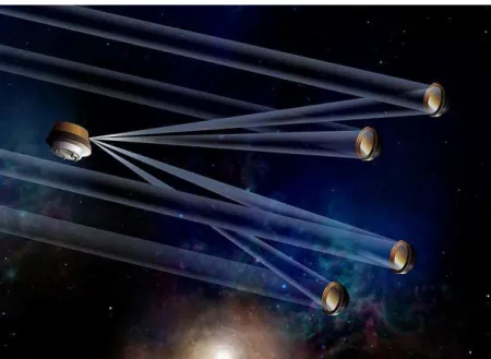
Darwin converged (Lawson et al. 2007). Fig.1.4shows an artist’s view of the space observatory which has to orbit the Sun with the same angular velocity as the Earth but at a distance 1.5 million km greater than the Earth, oscillating around the Sun-Earth L2 point. This positioning offers a number of advantages. Both the Earth and the Sun are always “behind” the spacecraft, facilitating cooling and observation planning. Less propellent is required for formation flying at L2 than in Earth orbit and even in an Earth-trailing orbit.
Figure 1.4 - Darwin/TPF-I space observatory. An artist’s view of the Emma X-array configuration with four telescopes. Each points in the direction of and receives light from the star-planet system. The four beams are transmitted to the central beam combiner which also provides, together with the communication station, metrological reference for the required formation flying. (Courtesy Peter R. Lawson, NASA/JPL.)
Search for biomarkers is a major factor when considering the spectral band. The values found are 6–20 µm. Regarding the diameter and number of telescopes, photometric, interferometric, and technical considerations lead to a trade-off of four 2 m apertures arranged in the so called Emma X-array.
Fig.1.5(Lawson and Dooley 2005) shows the provenance of the photons detected by Darwin/TPF-I. The figure shows the intensity of the local and exo-zodiacal emission, the leakage from the nulled star, and the background from the 35 K telescope. The resultant signal-to-noise ratio is shown on the right-hand scale. At 7 µm, the largest part of the measured flux is due to the star, then to the exozodiacal light, closely followed by local zodiacal light. The signal emitted (or reflected) by the planet is several orders of magnitude smaller.
Figure 1.5 - The signal in photo-electrons in a 105s integration period from an Earth-like planet
observed through the 1 AU, 3.5 m version of TPF. The planet shows CO2 absorption at 16 µm.
The spectral resolution is R=20. Also shown are the other signals that contribute to the total photon shot noise. The bottom curve shows the signal-to-noise ratio (SNR) on the planet using the right-hand scale. (Beichman et al. 1999)
The typical star-planet contrast that the instrument will need to operate with is 107. First, the nulling
must reduce the contrast by a factor 105.3 The whole observatory must rotate around the line of sight, maintaing a stable nulling level (Fig.1.6). A technique called phase chopping (or internal modulation) (Mennesson et al. 2005; Woolf and Angel 1997) is applied at the same time. The purpose of combining rotation and phase chopping is to distinguish between the centre-symmetric diffuse exozodiacal and the point-like planetary emissions (Fig.1.7). Together with instrument stability which enables long exposure times to reduce the noise (Sec. 1.3.3), this yields another factor 100, reaching 107 star-planet contrast reduction. An additional factor 10 can be obtained using the technique of spectral fitting (Lay 2006).
1.3.2
Nulling ratio
The output of a simple interferometer at any given moment is a single intensity measurement. Changing the optical path length of one beam with respect to the other (Optical Path Difference, OPD) leads to variations of intensity, i.e., when the OPD is scanned, a pattern of interference fringes emerges. Interference can only occur between beams which are coherent with respect to each other. Even beams generated by the same source may not be coherent if the OPD is too great: there is a certain coherence length to consider. A fringe pattern is observable around zero OPD, spanning the coherence length. The minima and maxima of the fringe pattern correspond to OPD’s of kλ/2 where k is even for the maxima and odd for the minima. The fringes can be circumscribed by an envelope symmetric around the zero OPD. The form of the envelope is given by a Fourier transform of the beam’s spectrum. Classical interferometry combines two coherent beams constructively. In order to do this, the beams have to be in phase. Then the fringe pattern’s global maximum is at zero OPD, and the fringes and the envelope have the same symmetry. Nulling interferometry inverses the fringes within the envelope, placing an interference minimum at its centre, i.e., at the zero OPD. This can be done by introducing a phase shift of π between the two interfering beams.
3This value is a result of a trade-off. Nulling reaches its nominal performance for on-axis light only, i.e., for light coming from a
12 1.3. FORMATION-FLYING NULLING INTERFEROMETER
Figure 1.6 - As the interferometer rotates around the line of sight to a target star, the planet (a 3R⊕ planet is shown for clarity in this TPF-I simulation) produces a modulated signal as it moves in and out of the interferometer fringe pattern. TPF would produce ≈ 20 such data streams, one for each of the observed wavelengths, that would be combined to reconstruct an image of the solar system and the spectra of any detected planets. (Beichman et al. 1999)
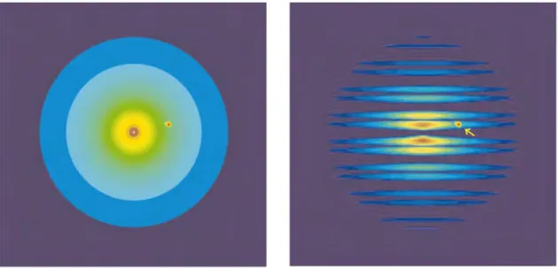
Figure 1.7 - The emission from a face-on exo-zodiacal dust cloud (left) with a single planet, and as it will be measured through the interferometer’s transmission pattern (right). (Beichman et al. 1999)
1.3.3
Stability
As already mentioned, because of the length of the planned exposure times during Darwin/TPF-I observa-tions, instrumental stability must be regarded as a serious concern.Chazelas et al.(2006), referring to this fact as to the variability noise condition, analyse the problem, stating that instrumental stability is required regardless of telescope size and stellar distance.
We have seen that although the star-planet contrast is of the order of 107
(4 × 10⁷at 7 µm in the case of
the Sun and the Earth), rotation & chopping techniques allow a reduction of the contrast by a factor 100, which means that the instrument has to provide a stable nulling ratio of 10−5(Eq.1.10). As pointed out
by Lay (Lay 2004), this implies a high degree of null stability. Let us examine the contributions to the instability of the signal, i.e., to the noise of Darwin/TPF-I measurements.
AppendixBcontains a discussion of these points because our work was to a large extent concerned with stability (Gabor et al. 2008a, cf. Chapter4). Here, let us merely present the result (Eq.B.10)
σhnli(λ, 10 days) ≤ 2.5 10−9 λ 7 µm
!−3.37
, (1.11)
which is expressed in terms of a quantity we shall define in Section2.2. In broad terms it can be interpreted if we recall the well-known truth of photography: the longer the exposure time, the sharper the picture. This is only true if the noise is of a certain sort. It is called the white noise, and it decreases with exposure time τ as √τ. The above Darwin/TPF-I requirement implies that the instrument noise has to be such that it allows for an improvement of the star-planet contrast over a period of 10 days.
4Sometimes also referred to as stellar leakage although this term refers more properly to stray starlight due to the fact a star is not
2.3 Achromatic Phase Shifters . . . 18
2.4 The Dispersive Prisms APS . . . 20
2.5 Wavefront filtering. . . 20
2.6 Stability. . . 22
2.7 State of the art. . . 23 In the previous Chapter (1), we saw that nulling interferometry is a promising approach in future re-search on exoplanets and astrobiology. We described, in very broad lay terms, the principle of Darwin/TPF-I. We listed the mission’s main requirements imposed on the nulling interferometer itself (Eqs.1.10,B.10), deriving the requirement Eq.B.10in detail.
The purpose of this Chapter is to discuss two-beam nulling interferometers and their components.
2.1
Bracewell’s principle
Interferometry is primarily a technique the purpose of which is angular-resolution improvement. Without having to resort to prohibitively large apertures, a classic two-aperture interferometer can increase angular resolution by separating two smaller telescopes by a certain distance, called base B. The beams collected by the individual apertures have to be combined under carefully controlled conditions. The interference pattern is then analysed and spatial or angular information about the target can be obtained. In order to obtain an image, it is necessary to perform a series of measurements with different lengths and orientations of the base, densely covering the parameter space.
Each measurement is done with the telescopes aligned and observing the same object. We ensure that the on-axis light from both telescopes arrives simultaneously, i.e., the two optical paths are equal, to the beam-combiner system where it merges on a single-element detector.1 The output is therefore a single value.
A set of such measurements for various values of Optical-Path Difference (OPD) forms an interference pattern. The zero OPD difference corresponds to the interference maximum, known as the white fringe. In theory, the white fringe does not have an intensity which would be just the sum of the intensities of the two interfering beams: its intensity is double the sum, i.e., four times the intensity of one interfering beam. This
16 2.2. PERFORMANCE PARAMETERS
Figure 2.1 - Bracewell’s nulling interferometer: two telescopes pointing in the direction of the star, the light of which is extinguished using an achromatic phase shifter (+π) so that the bright-ness contrast between the star and the planet is reduced.
is possible because in case of perfect interference of two monochromatic beams, there is strictly no flux at the interference minima. Thus the mean value of the flux is the expected sum of the two incident beams.
In the case of natural light (broad band), the white fringe, which corresponds to zero OPD, is still well defined, but the interference minima occur at different values of OPD for different wavelengths. This gives the interference pattern the characteristic shape of a packet of fringes: each successive fringe less and less pronounced.
A variant of this technique was proposed byBracewell(1978). Instead of combining the beams con-structively, he proposed to combine them destructively. The zero OPD corresponds to the interference minimum, known as the dark fringe. While this is trivial in the case of monochromatic light, natural light cannot be combined destructively unless an achromatic (wavelength-independent) phase shift is introduced. Supposing we have a perfectly achromatic phase shifter that shifts the phase of one of the beams by π, we obtain an inversion of the interference pattern. The dark fringe is symmetrically surrounded by imperfect white fringes, called grey fringes. The on-axis light is combined destructively. This property of the nulling interferometer makes it the instrument which can increase angular resolution and reduce the star-planet contrast.
In its simplest form (Fig.2.1), a two-telescope nulling interferometer introduces a π phase-shift between the two apertures, resulting in destructive interference along the line of sight. At the same time, light at small off-axis angles from the line of sight will experience constructive interference, thus allowing a faint object close to a bright star to be discernible.
2.2
Performance parameters
Let us recall the quantities used in characterising the performance of nulling interferometers.
Nulling ratio was defined in Eq.1.9as
nl(λ, τ) = Imin
averages hnliτ, each averaged over exposure time τ, and calculate its standard deviation σhnli(τ). Now,
repeat the procedure for a number of different windows widths τ, and inspect the dependence of σhnli(τ) upon τ. If it is consistent with τ−1/2(i.e., white noise behaviour) up to a certain τmax, then
σhnli(τ = τmax) (2.4)
is a good expression of the nuller’s stability.
Rudiments of interferometry. In the simplest, monochromatic case, we can represent a single wave with an amplitude of A as a function of the phase φ:
S1= A1eiφ1, (2.5)
and the corresponding intensity I1is:
I1= |A1|2. (2.6)
Let us make two such waves interfere. The resulting complex sum is:
S = S1+ S2= A1eiφ1+ A2eiφ2, (2.7)
and the intensity I is
I = |A1|2+ |A2|2+ 2|A1||A2| cos(φ1− φ2), (2.8)
which can be expessed as
I = I1+ I2+ 2
p
I1I2cos(φ1− φ2). (2.9)
If I1= I2, the interference pattern’s maximum, Imax, corresponds to |φ1− φ2| = 0, i.e.,
Imax= 2I1+ 2I1cos(0) = 4I1, (2.10)
whereas the minimum, Imin, corresponds to |φ1− φ2| = π, i.e.,
Imin= 2I1+ 2I1cos(π) = 0, (2.11)
hence the nulling ratio is
nl = Imin
Imax = 0. (2.12)
Let us examine the behaviour of the nulling ratio close to this value, i.e., for |φ1− φ2| = ∆φ ≪ 1. In this
case we obtain nl = Imin Imax = 1 + cos(π + ∆φ) 1 + cos(∆φ) = 1 − cos(∆φ) 1 + cos(∆ϕ) (2.13)
18 2.3. ACHROMATIC PHASE SHIFTERS nl ≈ 1 − 1 + ∆φ2 2 1 + 1 −∆φ22 ≈ ∆φ 2 4 for ∆φ ≪ 1. (2.14)
Let us now return to the situation where |φ1− φ2| = 0, and examine what happens if I1 ,I2. Supposing
I2= (1 + ǫ)I1, (2.15)
where ǫ ≪ 1. This means that the relative flux flux mismatch ∆I/I is ∆I I = I2− I1 I1 = (1 + ǫ)I1− I1 I1 = ǫI1 I1 = ǫ. (2.16)
The nulling ratio nl then is
nl = Imin Imax =I1+ I2+ 2 √ I1I2cos(π) I1+ I2+ 2 √ I1I2cos(0) = I1+ I2− 2 √ I1I2 I1+ I2+ 2 √ I1I2 , (2.17) nl = I1+ (1 + ǫ)I1− 2I1 √ 1 + ǫ I1+ (1 + ǫ)I1+ 2I1 √ 1 + ǫ = 2 + ǫ − 2 √ 1 + ǫ 2 + ǫ + 2√1 + ǫ, (2.18) developing √1 + ǫ: √ 1 + ǫ = 1 + ǫ 2 − ǫ2 8 + ... (2.19) nl ≈ 2 + ǫ − 2(1 + ǫ 2− ǫ2 8) 2 + ǫ + 2(1 + ǫ2−ǫ82) = −2−ǫ82 4 + 2ǫ + 2−ǫ82, (2.20) nl ≈ ǫ 2 16. (2.21)
2.3
Achromatic Phase Shifters
One of the key components of the Bracewell interferometer is the Achromatic Phase Shifter (APS). It is an optical element designed to introduce a given difference in phase in a beam regardless of the wavelength.
Let us state clearly that in real life there are no perfect optical elements that would fulfil this function ideally. There are many workable solutions, however, always representing a compromise between the “neatness” of the phase shift (how well does the real phase shift correspond to the required value), and the width of the spectral band in which it is to be achieved.
For a given Optical-Path Difference (OPD) between the two optical paths, the corresponding phase difference ∆ϕ can be expressed as
∆ϕ = 2πOPD
λ , (2.22)
where λ is the wavelength.
The phase shift therefore depends on the wavelength, ∆ϕ = ∆ϕ(λ). In order to obtain a wavelength-independent phase shift of π at zero OPD, an APS has to be introduced into the setup.
There are alternative approaches, however. The “adaptive nuller” was tested at the JPL (Peters et al. 2008), and at Delft, polarisation and multi-axial nulling interferometry were studied (Spronck et al. 2006). Many different concepts of achromatic phase shifters are available in the literature (Rabbia et al. 2001, 2000). The Darwin collaboration studied ten APS concepts (ESA 2002), promising nl < 10−6. The spectral range was that of 6–20 µm, with 6–18 µm mandatory, the extension to 18–20 µm priority number 2, and that to 4–6 µm priority number 3. Their various merits will eventually need to be evaluated experimentally. Not all of these concepts are currently in the research and development process. Some, although promising
(c) Focus Crossing or Through Focus (d) Fresnel’s Rhombs
Figure 2.2 - The four APS concepts investigated by ESA.
in the long run, require a substantial effort to overcome technical hurdles chiefly because of the novelty and of the required spectral range (e.g., integrated optics, zero order gratings).
Out of the ten, four APS concepts were selected for further study by ESA in recent years (Fig.2.2):
1. Dielectric or Dispersive Prisms,
2. Focus Crossing or Through Focus, 3. Field Reversal or Periscope, and 4. Fresnel’s Rhombs.
The S testbed uses two pairs of CaF2 Prisms (Sec.3.11) as a Dispersive Prisms APS and, at
the same time, the prisms form an intrinsic part of the setup because they also function as a compensator balancing the cumulative thickness of dielectric in the optical path.
A Dispersive Prisms APS prototype with three pairs of prisms of three different materials was developed by Thales Alenia Space (Sec.3.9.3). A Focus Crossing APS prototype was designed by the Observatoire de Cˆote d’Azur, Nice, France (Sec.3.9.1). And, last but not least, a Field Reversal APS prototype was manufactured at Max-Planck-Institut f¨ur Astronomie in Heidelberg in collaboration with Kayser-Threde GmbH in Munich and the IOF Fraunhofer Institute for Applied Optics in Jena (Sec.3.9.2).
20 2.4. THE DISPERSIVE PRISMS APS
2.4
The Dispersive Prisms APS
Let us now look in more detail at the Dispersive Prisms APS because it of its rˆole in the S setup. This method is directly inspired by the practice of opticians who try to minimise chromatic aberrations in lens systems.
We shall examine one of the simplest cases when a pair of dispersive prisms is introduced into each arm of the interferometer. The beams thus propagate in two different media, viz., in air and in the dielectric. The refractive index ndielof the dielectric varies with wavelength,
ndiel= ndiel(λ). (2.23)
We shall consider air as not dispersive, i.e., its index nairdoes not vary with wavelength
nair(λ) = 1. (2.24)
Because of the presence of the dispersive elements, the phase difference ∆φ between the two beams will vary with wavelength
∆φ = ∆φ(λ). (2.25)
It can be expressed as
∆φ(λ) = 2π
λ [nair· (OPD + e) − e · ndiel(λ)] , (2.26) where e is the difference in thickness of dielectric encountered by the beams. Note that we can consider the total geometric length of the optical path constant, i.e., adding dielectric into the optical path reduces the air column in it by the same amount. We can thus write
∆φ(λ) = 2π
λ [OPD · nair+ e · (nair− ndiel(λ))] . (2.27) Now we can impose
∆φ(λ1) = π, (2.28)
∆φ(λ2) = π, (2.29)
for two distinct wavelengths λ1,2. This is a set of two equations with two unknowns, e and OPD,
2π
λ1 [OPD · n
air+ e · (nair− ndiel(λ1))] = π, (2.30)
2π
λ2 [OPD · n
air+ e · (nair− ndiel(λ2))] = π. (2.31)
For given two wavelengths there are values of e and OPD which correspond to a perfect nl = 0. If the material and the waveband are chosen appropriately, a Dispersive Prisms APS can provide nulling better than a specified value within the waveband (Fig.2.3).
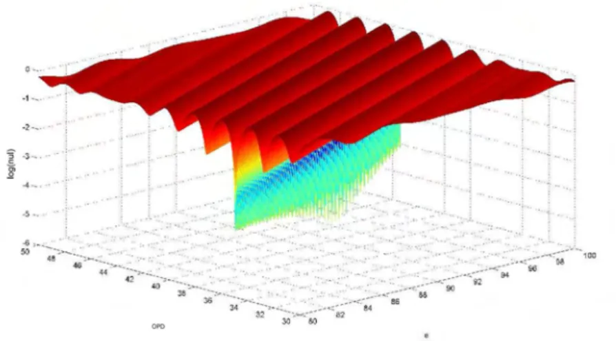
Let us look at the dual problem: How do we find the working point if we have the means to explore the parameter space (OPD, e)? Fig.2.4shows that there are many local minima, and thus we need to understand this space better in order to find the global minimum. Performing an OPD scan for a given value of e will yield a fringe packet. If the fringe packet is symmetric, we find a minimum (Fig.2.5). It could be a local minimum, however. The ambiguity can be lifted by looking at neighbouring minima. Section6.1.5 describes a practical application of this technique.
2.5
Wavefront filtering
Another important ingredient in nulling interferometry is wavefront filtering. Achieving high levels of destructive interference implies stringent requirements in terms of wavefront quality. These requirements can be reduced using a wavefront filter (Mennesson et al. 2002).
Figure 2.3 - Nulling ratio as a function of wavelength (in µm) produced by Dispersive Prisms APS with two thicknesses of CaF2, one per beam. Appropriate selection of thicknesses ensures
that in a given spectral band (highlighted) the nulling ratio is nl < 10−4. This is possible because CaF2is dispersive, i.e., its refractive index varies with wavelength.
Figure 2.4 - Map of the (OPD, e) space. There are many local minima in the (OPD, e) parameter space. Nonetheless, the global minimum is unique.
22 2.6. STABILITY
Figure 2.5 - Three OPD scans for different values of e. Performing an OPD scan for a given value of e will yield a fringe packet. If the fringe packet is symmetric, we find a minimum. It could be a local minimum, however. The ambiguity can be lifted by looking at neighbouring minima.
1. Pinholes, i.e., spatial filters;
2. Single-Mode optical Fibres (SMF’s), i.e., modal filters.
A SMF is, effectively, a waveguide that transmits only one resonance mode. We can view the fibre as a resonance cavity with a single resonance mode in the given spectral band. This resonance mode is a solution of Maxwell’s equations and is not confined to the internal volume of the fibre. In fact, it extends from both extremities of the fibre as lobes. Therefore, whatever the properties of the optical field incident upon the fibre head, the output of the fibre will be an extension of this proper mode.
Nulling interferometers require that the wavefront be without distortion to a level of λ/1000 if the nulling ratio nl is to be less than 10−5(Sec.3.3.6). The reason is easily seen when we realise that if there
are defects in the wavefront, a part of the flux arrives at the point of interference out of phase. Without wavefront filtering, the λ/1000 requirement would be prohibitively strict because it implies that all the optical surfaces must be polished to that level of precision.
Unfortunately, the only way to estimate the quality of SMF’s is to measure it with a specialised nulling interferometer (Ksendzov et al. 2007).
2.6
Stability
Experimental studies of nulling interferometer testbeds (Serabyn 2003;Schmidtlin et al. 2005;Ollivier et al. 2001;Vink et al. 2003;Alcatel;Brachet 2005) show that even in simple setups, the interference pattern is unstable, drifting with time. Even interferometers breadboarded on an optical bench in the relatively well-controlled laboratory environment (a priori simpler than the actual Darwin/TPF-I, with its multiple tele-scopes rotating in space) display drifts.Chazelas et al.(2006) give a quantitative summary of these effects, using data fromOllivier(1999);Alcatel;Vink et al.(2003).
demonstrated 4-beam nulling with nl = 4 × 10⁻⁶and the detection of a simulated planet at a contrast level of 2 × 10⁶(Martin et al. 2006).
24 2.7. STATE OF THE ART
0.0 0.1 0.2 0.3 0.4 0.5
Bandwidth / central wavelength 10-7 10-6 10-5 10-4 10-3 10-2 Null Depth Bokhove 2003 Bokhove 2003 Bokhove 2003 Brachet 2005 Gabor 2008 Gabor 2008 Buisset 2006 Buisset 2006 Weber 2004 Morgan 2003 Vosteen 2005 Schmidtlin 2005 Schmidtlin 2005 Tavrov 2005 Flatscher 2003 Flatscher 2003 Ollivier 1999 Ollivier 1999 Martin 2003 Mennesson 2003 Mennesson 2003 Wallace 2004 Mennesson 2006 Gappinger 2009 Gappinger 2009 Gappinger 2009 Gappinger 2009 Gappinger 2009 Samuele 2007 Samuele 2007 Wallace 2000 Labadie 2007 Peters 2008 Visible H band K band N band Laboratory Nulling Results 1999-2009
0.00 0.01 0.02 0.03 0.04 0.05 0.06 0.07
Bandwidth / central wavelength 10-6 10-5 Null Depth Bokhove 2003 Gabor 2008 Buisset 2006 Weber 2004 Martin 2003 Martin 2003 Wallace 2003 Schmidtlin 2005 Schmidtlin 2005 Flatscher 2003 Flatscher 2003 Martin 2003 Martin 2003 Martin 2005 Haguenauer 2006 Gappinger 2009 Gappinger 2009
Zoom on Laser Nulling Results
Figure 2.6 - Chart of nulling ratios achieved in laboratory experiments. The plot summarises the best results reported in the indicated papers, plotting the null depth against the bandwidth (given as a fraction of the central wavelength). The unabridged bibliographical references are provided in Table2.1. Bottom plot provides a zoom on the narrow-band and laser experiment sector.
2.1 × 10
650 nm 0.05 8.3 × 10⁻⁶ + Schmidtlin et al.(2005) Opt. Pl. Det. Int., JPL
650 nm 0.12 3.2 × 10⁻⁵ + Schmidtlin et al.(2005) Opt. Pl. Det. Int., JPL
650 nm 0.15 1 × 10⁻⁶ – Samuele et al.(2007) Northrop, Redondo B.
650 nm 0.18 7.1 × 10⁻⁵ + Wallace et al.(2000) JPL
700 nm 0.28 7 × 10⁻³ – Morgan et al.(2003) Nulling B. Comb., JPL
1306 nm 8 × 10⁻⁵ 2.5 × 10⁻⁶ – Flatscher et al.(2003) Astrium, Friedrichshafen
1.54 µm 3 × 10⁻⁶ 1.3 × 10⁻⁶ + Weber(2004) MAII I, Cannes
1.545 µm 0.02 3.1 × 10⁻⁵ – Flatscher et al.(2003) Astrium, Friedrichshafen
1.55 µm 0.05 2.7 × 10⁻⁵ – Buisset et al.(2007) MAII II, Cannes
1.55 µm 0.05 6 × 10⁻⁶ + Buisset et al.(2007) MAII II, Cannes
1.55 µm 1 × 10⁻³ 4.3 × 10⁻⁶ – Flatscher et al.(2003) Astrium, Friedrichshafen
1.57 µm 0.05 1.7 × 10⁻⁴ – Weber(2004) MAII I, Cannes
1.65 µm 0.18 5 × 10⁻⁴ – Mennesson et al.(2006) Fiber Nuller, JPL
2.2 µm 0.18 2.5 × 10⁻⁴ – Brachet(2005) S I; IAS Orsay
3.39 µm 3 × 10⁻⁶ 1 × 10⁻⁵ + Gabor et al.(2008c) S II; IAS Orsay 3.39 µm 3 × 10⁻⁶ 1 × 10⁻⁴ – Gabor et al.(2008c) S II; IAS Orsay 9.5 µm 0.2 2 × 10⁻⁵ + Gappinger et al.(2009) Achr. Nulling T., perisc. 9.5 µm 0.25 4 × 10⁻⁵ + Gappinger et al.(2009) Achr. Nulling T., perisc.
9.5 µm 0.25 6.7 × 10⁻⁴ – Gappinger et al.(2009) Achr. Nulling T., FC
9.5 µm 0.30 9.1 × 10⁻⁵ – Gappinger et al.(2009) Achr. Nulling T., 2Prism
9.5 µm 0.30 8.8 × 10⁻⁵ – Gappinger et al.(2009) Achr. Nulling T., 1Prism
10 µm 0.30 1 × 10⁻⁴ – Wallace et al.(2004) Warm Nulling Testbed, JPL
10 µm 3 × 10⁻⁶ 3.3 × 10⁻⁶ + Gappinger et al.(2009) Achr. Nulling T., perisc.
10 µm 3 × 10⁻⁶ 1.1 × 10⁻⁵ – Gappinger et al.(2009) Achr. Nulling T., perisc.
10 µm 0.4 1 × 10⁻⁵ + Peters et al.(2008) Adaptive Nuller T., JPL
10.6 µm 3 × 10⁻⁶ 1 × 10⁻³ – Ollivier(1999) IAS Orsay; typ.
10.6 µm 3 × 10⁻⁶ 7 × 10⁻⁴ – Ollivier(1999) IAS Orsay; best
10.6 µm 3 × 10⁻⁶ 1.1 × 10⁻⁶ – Martin et al.(2003a) MMZ Nuller, JPL
10.6 µm 3 × 10⁻⁶ 7 × 10⁻⁷ + Martin et al.(2003a) MMZ Nuller, JPL
10.6 µm 3 × 10⁻⁶ 7.3 × 10⁻⁶ – Martin et al.(2005) Planet Detection T., JPL
10.6 µm 3 × 10⁻⁶ 5.6 × 10⁻⁵ – Labadie et al.(2007) Grenoble
10.675 µm 0.18 5.9 × 10⁻⁵ – Mennesson et al.(2003) Keck Nuller B. Comb., JPL 10.775 µm 0.29 1.3 × 10⁻⁴ – Mennesson et al.(2003) Keck Nuller B. Comb., JPL
Table 2.1 - Main nulling-interferometry laboratory results, ordered according to spectral band (first column). The second column gives the bandwidth (as a fraction of the central wavelength), the third column give the best null achieved, the “Pol” column indicates whether polarisers were used at the output. The “Reference” and “Experiment” columns indicate the setup (“Achr. Nulling T.” is the Achromatic Nulling Testbed at the JPL which had several phase shifter options: “perisc.” was the periscope, “FC” was the through focus or focus crossing, “1Prism” was a setup with ZnSe dispersive prisms, “2Prism” was a setup with ZnSe and ZnS prisms).
3.1.2 General note . . . 28
3.1.3 Historical background . . . 29
3.2 General overview . . . 32
3.2.1 An outline. . . 32
3.2.2 General layout . . . 33
3.3 Purpose of the subsystems. . . 36
3.3.1 A point source observed by two apertures . . . 36
3.3.2 Three remarks on single-mode fibres. . . 36
3.3.3 Off-axis parabolic mirrors . . . 37
3.3.4 Symmetry. . . 38
3.3.5 Flux balancing . . . 40
3.3.6 Stability. . . 41
3.3.7 Optical path. . . 43
3.4 Sources . . . 44
3.4.1 Ceramic black body . . . 44
3.4.2 3.39 µm HeNe laser . . . 46
3.4.3 Supercontinuum laser source. . . 46
3.4.4 2.32 µm laser diode. . . 47
3.5 Modal filters . . . 48
3.5.1 Fluoride-Glass Single-Mode Fibres . . . 48
3.5.2 Fibre output aperturing . . . 48
3.6 Spectral filters . . . 48
3.7 Polarisers . . . 50
3.8 Detectors . . . 50
3.8.1 Array detector . . . 50
3.8.2 Single element detector. . . 50
3.9 Phase shifter prototypes. . . 53
3.9.1 Focus Crossing or Through Focus . . . 53
3.9.2 Field Reversal or Periscope. . . 53
3.9.3 Dispersive prisms. . . 54