Reconstructing modern and past weathering regimes using boron isotopes in river sediments

(1)

HAL Id: tel-02176267

https://tel.archives-ouvertes.fr/tel-02176267

Submitted on 8 Jul 2019

HAL is a multi-disciplinary open access archive for the deposit and dissemination of sci-entific research documents, whether they are pub-lished or not. The documents may come from

L’archive ouverte pluridisciplinaire HAL, est destinée au dépôt et à la diffusion de documents scientifiques de niveau recherche, publiés ou non, émanant des établissements d’enseignement et de

Reconstructing modern and past weathering regimes

using boron isotopes in river sediments

Christian Ercolani

To cite this version:

Christian Ercolani. Reconstructing modern and past weathering regimes using boron isotopes in river sediments. Geochemistry. Université de Strasbourg; University of Wollongong (Wollongong, Australie), 2018. English. �NNT : 2018STRAH008�. �tel-02176267�

(2)

UNIVERSITÉ DE STRASBOURG

École Doctorale des Sciences de la Terre et de l’Environnement

Laboratoire d’Hydrologie et de Géochimie de Strasbourg (LHyGeS)

THÈSE

présentée par :

Christian ERCOLANI

soutenue le : 25 septembre 2018

pour obtenir le grade de :

Docteur de l’université de Strasbourg

Discipline/ Spécialité

: Géochimie

Reconstruction des régimes d’altération actuels et

passés à partir des isotopes du bore dans les sédiments

de rivière

THÈSE dirigée par :

LEMARCHAND Damien MCF, HDR, Université de Strasbourg

DOSSETO Anthony Associate Professor, University of Wollongong

RAPPORTEURS :

NÄGLER Thomas Professor, Universität Bern

PUCÉAT Emmanuelle MCF, HDR, Université de Bourgogne

EXAMINATEURS :

CHABAUX François Professeur, Université de Strasbourg

(3)

Reconstruction of modern and past weathering regimes using

boron isotopes in river sediments

Christian Paul Ercolani

Supervisors: Dr. Anthony Dosseto Dr. Damien Lemarchand

This thesis is presented as part of the requirement for the conferral of the degree: Doctor of Philosophy

The University of Wollongong School of Earth and Environmental Science

(4)

Christian ERCOLANI

Reconstruction of modern and

past weathering regimes using

boron isotopes in river

sediments

Résumé

Cette thèse a les objectifs suivants :

1. Mieux comprendre comment les isotope du bore dans les sédiments fluviaux modernes enregistrent le régime d’altération à la échelle du bassin versant.

2. Mieux comprendre comment le « signal » d’altération porté par les sédiments fluviaux est transféré des zones sources vers l’environnement de dépôt.

3. Déterminer si les isotopes du B dans les dépôts sédimentaires (paléo-canaux) peuvent être utilisés pour reconstituer les conditions paléo-climatiques et paléo-environnementales et ainsi révéler

comment l’altération continentale au sens large (production et transport de sédiments) a réagi à la variabilité climatique au cours du dernier cycle glaciaire-interglaciaire (derniers 100 ka).

Ces objectifs ont été examinés en étudiant les matériaux fluviaux des fleuves Gandak (Himalaya) et Murrumbidgee (NSW, Australie) et des dépôts de sédiments fluviaux de la Riverine Plain (bassin versant de Murrumbidgee, Australie). La connaissance des paramètres qui contrôlent le

fractionnement isotopique du bore des sédiments fluviaux au cours de la formation et du transport a d'abord été acquise dans les systèmes modernes, puis appliquée à d'anciens dépôts de

paléochenaux.

Résumé en anglais

This thesis has the following objectives:

1. To better understand how boron isotopes in modern fluvial sediments record the weathering regime at the catchment scale.

2. To better understand how the weathering “signal” carried by river sediments is transferred from source areas to the depositional environment.

3. To determine if boron isotopes in sediment deposits (paleochannels) can be used to reconstruct paleo-weathering and paleo-environmental conditions and reveal how continental weathering at large (production and sediment transport) responds to climatic variability over the last glacial-interglacial cycle (approximately the last 100 ka).

These objectives were addressed by studying fluvial material from the Gandak (Himalayas) and Murrumbidgee (NSW, Australia) Rivers and fluvial sediment deposits from the Riverine Plain (Murrumbidgee catchment, Australia). Knowledge of the parameters that control boron isotope

(5)

ABSTRACT

Chemical weathering coupled with carbonate precipitation in the oceans is largely responsible for the sequestration of atmospheric CO2, which balances CO2 inputs into the atmosphere from

mantle degassing and thus participates in the global climate regulation at the geological time scale. Despite the importance of chemical weathering in maintaining habitable conditions on the Earth's surface, quantification of past and present chemical weathering remains difficult. The intensity of modern chemical weathering is generally determined from the geochemistry of solutes and sediments transported by rivers. However, this approach suffers from the lithological control on the composition of the dissolved load and granulometric/mineralogical sorting during sediment transport. Alternatively, boron (B) isotopes have physicochemical properties suitable to study of water-rock interactions, including those involving a biological component. The processes responsible for B isotope fractionation are adsorption on clay and detrital particles, precipitation in secondary phases, and recycling through vegetation. While several studies have used B isotopes as a proxy to quantify chemical weathering reactions in the dissolved load of rivers, few have focused on river sediments. As a result, the parameters that control B isotope behavior during the production of secondary products and subsequent transport from source areas to the deposition environment are not fully understood. Additionally, the use of B isotopes as potential proxy for weathering and paleo-environment reconstruction is relatively unknown. In the Gandak River (Himalayas) suspended and river bank sediments were collected along the course of the river in order to better understand the parameters that control B isotope fractionation in sediments transported by rivers. Grain size fractions were analyzed for B isotopes and major and trace element ly fractionated with respect to the primary minerals, represented by the sand fraction (63 µm - 2 mm), and evolve downstream, while all other size fractions have a constant composition. The downstream evolution of B isotope compositions and concentrations in the clay fraction reflect differences in the weathering regime; dissolution reactions are dominant in the headwaters, while secondary phase precipitation reactions dominate downstream. Similarly, bank sediments and the dissolved load of the Murrumbidgee River and its tributaries (NSW, Australia) were analyzed to assess the role of lithology, climate, and geomorphology on B isotope fractionation in weathering products and their transport from source areas to the depositional environment.

(6)

Boron isotopes in the clay fraction of bank sediments also show an increase in isotope ratios downstream in the watershed, a behavior attributed to changes in the weathering regime in sediment production areas. The B isotope composition of clay fractions is disconnected from that of the dissolved load of the river, which reflects both an absence of isotopic exchange during transport and a disconnection between the fluid that produces the clay and the fluid that composes the dissolved phase of the river. A mass balance model reveals that the composition of the clay fraction represents a mixture of sediment sources throughout the watershed. Therefore, no chemical or isotopic evolution of the sediments was observed during transport. Paleochannel sediments in the Murrumbidgee catchment were also analyzed for boron and neodymium (Nd) isotopes, major and trace element concentrations, and sediment mineralogy. After identification and removal of samples which were affected by post-depositional alteration, distinct B isotope variations between paleochannel systems can be made. This B isotope record in the paleochannels correlates with a sea surface temperature (SST) and vegetation cover records over the last 100 ka indicating that clay formation in source areas has responded to climatic variability, particularly temperature and vegetation cover. During warmer and wetter periods (Marine Isotope Stages 1, 3, and 5), the role of vegetation on pedogenesis is greater than during colder periods (Marine Isotope Stage 2). Finally, Nd isotopes in the clay fraction show that there has been no significant change in sediment provenance for the last 100 ka. These results highlight the potential for the use of B isotopes to quantify modern and past weathering regimes, including their use in sediment deposits as a proxy to reconstruct paleo-weathering and paleo-environmental conditions.

(7)

ACKNOWLEDGEMENTS

The opportunity to earn a doctoral degree comes but once in a life time. Success is not measured by how much you achieve, but rather how many times you attempt to achieve success. Hardships and mishaps are just part of the experience, which in the end, often lead to much better and interesting results. Patience and perseverance are two skills I learned through the undertaking of this degree; skills I will use the rest of my life. I would like to thank my PhD supervisors, Drs. Anthony Dosseto and Damien Lemarchand for their continual guidance, wisdom, and support they have given me throughout every step of this process. Without their oversight and encouragement, this project would not have reached its full potential. Likewise, my potential as a scientist may not have been realized.

I would like to thank both the University of Wollongong and the Université de Strasbourg for providing matching post-graduate scholarships which made this research possible. I would also like to thank both institutions for hosting me and giving access to their fine laboratory equipment and space. This includes the assistance from lab technicians Lili Yu, José Abrantes, Thierry Perrone, Mathieu Granet, René Boutin and Professors Brian Jones and Tim Cohen. I would like to thank my PhD colleagues who have helped with my work, both in the field and lab, including Philippe Roux, Leo Rothacker, Ashley Martin, and Gabriel Enge.

I also give many thanks to my family, especially my parents, who have provided continual love and support, not only through this process but throughout my life. They taught me to make my dreams a reality, which is what I did.

I would like to thank my colleagues and friends I’ve made along this journey for their support, encouragement, and guidance during this difficult time. It was great to have these wonderful people in my life.

Finally, I truly may not have made it without the endless love and support of my partner, Andrew, who undertook this adventure with me. With you by my side, I know anything is possible. You are my rock.

(8)

TABLE OF FIGURES

Figure 1-1. A model of the long-term carbon cycle (Berner 2003) ...19 Figure 1-2. Arrhenius diagrams of the log Si effluent concentrations from both fresh and

weathered granitoid rocks (White et al. 1999)...21 Figure 1-3. Total dissolved solids vs. runoff for rivers worldwide. (Holland 1978)...25 Figure 1-4. Ice core data from Vostok, Antarctica (Petit et al. 1999)...32 Figure 1-5. Chemical Index of Weathering (CIW), Chemical Index of Alteration (CIA), and

Plagioclase Index of Alteration (PIA) taken from a weathering profile consisting of bedrock and saprolite (Price and Velbel, 2003)...41 Figure 1-6. Relationships between the fluxes of material coming from chemical weathering of

silicates and a) the fluxes of cations from the weathering of silicate material and b) the flux of CO2removed from the atmosphere from weathering attributed to aluminosilicate

weathering (Gaillardet et al. 1999) ...45 Figure 1-7. Evolution of the normalized mobile elements composition (relative to Si) of

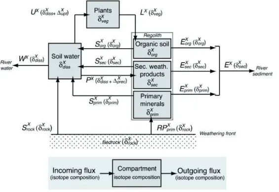
Himalayan sediments (Lupker et al. 2012) ...47 Figure 1-8. Conceptual diagram of an Al-normalized soluble element concentration (X/Al)

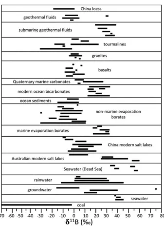
used as a weathering index, as function of Al/Si, used as a grain size proxy (Bouchez et al. 2013) ...49 Figure 1-9. Schematic diagram of the weathering zone model (Bouchez et al. 2013) ...55 Figure 1-10. Boron isotopic compositions in nature (Xiao et al. 2013) ...58 Figure 1-11. a) Boron adsorption distribution coefficient as a function of pH (Palmer et al.

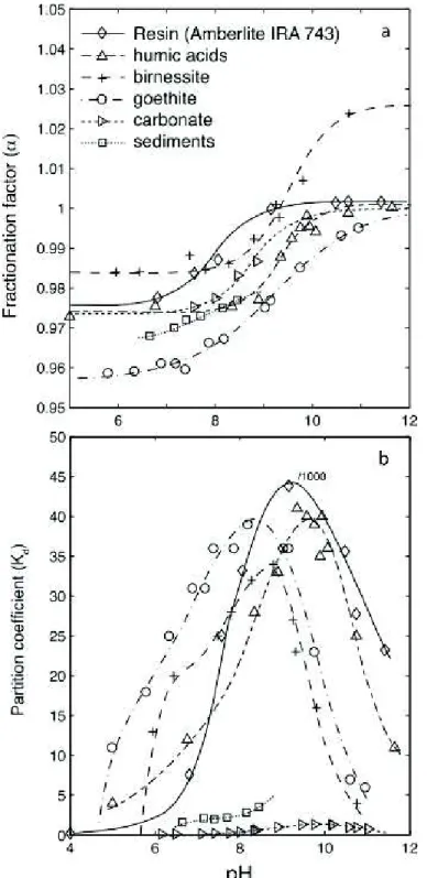
1987) ...61 Figure 1-12. Kd – pH and – pH relationships for different geology and synthetic material.

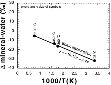
...63 Figure 1-13. Boron isotope fractionation as a function of reciprocal temperature ...66 Figure 1-14. B/Ti* (a) and 11B in bulk soil samples as a function of depth taken in the

Strengbach forest catchment (France) (Lemarchand et al. (2012)...70 Figure 1-15. Published boron isotopes compositions in bulk soils as function of the Al/Si

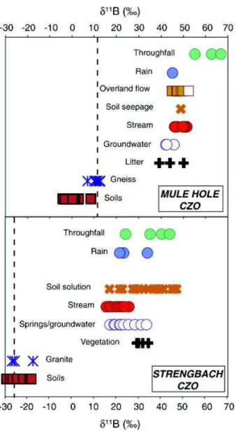
ratio in different soil profiles (Gaillardet and Lemarchand (2017)...72 Figure 1- 11_{B values in the different compartments of two contrasted Critical Zone}

Observatories, Mule Hole basin, India and Strengbach basin, France ...74 Figure 1-17. Modelled changes in B isotopes in Himalayan soil porewaters during weathering

processes as a function of water pH (Rose et al. 2000) ...76 Figure 1-18. Boron isotope compositions as a function of B concentrations for Réunion

Island rivers and springs ...78 Figure 1-19. Modeled temporal evolution of the B isotope ratio in shallow groundwaters in

the Mackenzie River basin in response to changes in the weathering conditions (caused by past glacial events) ...81 Figure 1-20. Evolution of the 11B solid-dissolved as a function of the Al/B mass ratio

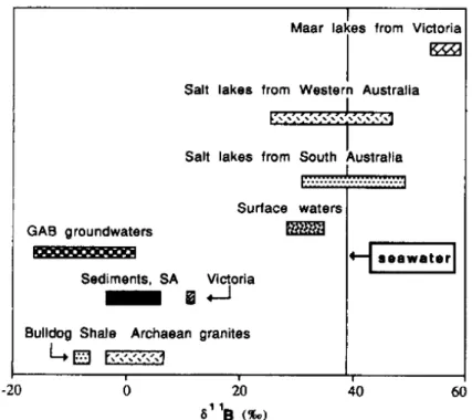
measured in suspended sediments of the Changjiang basin rivers ...82 Figure 1-21. 11B compositions in some Australian brines, surface waters, groundwaters,

sediments, and bedrock ...83 Figure 2-1. Lithology and digital elevation map (DEM) of the upper Murrumbidgee River

and tributaries displaying sampling points for sediments and water (black dots) and sampling points for sediment, water, and bedrock in monolithological catchments with respective drainage catchment areas (hashed areas)...90

(12)

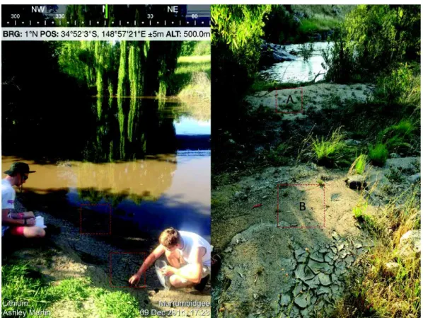
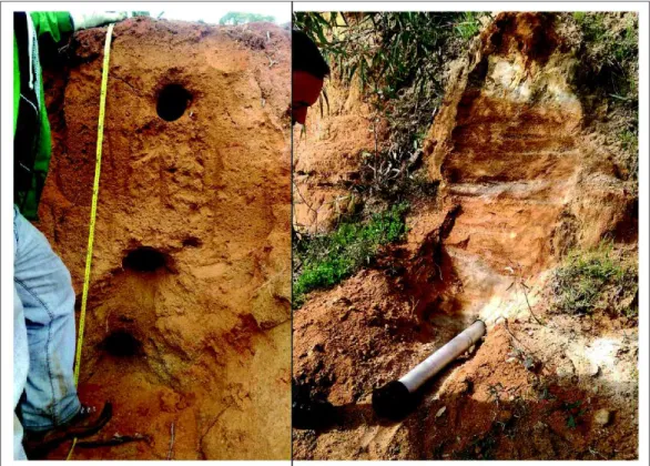
Figure 2-2. Examples of river sediment collection on the river bank of the Murrumbidgee River...91 Figure 2-3. River water sample taken from the middle of the stream (Murrumbidgee)...92 Figure 2-4. Paleochannel sediment deposit profiles showing sampling strategy ...94 Figure 2-5. XRD diffraction pattern of a clay fraction sample showing the non-glycol (green) diffraction patter overlain by the glycol (red) diffraction pattern...95 Figure 2-6. XRD diffraction pattern of a clay fraction sample being quantified by the

SIROQUANT software...96 Figure 2-7. Components of the MC ICP-MS Neptune Plus (Thermo Fisher Scientific)...108 Figure 2-8. Typical peak shape measured on mass 11 after tuning in a 50 ppb NIST 951

solution during an analytical session on the Neptune Plus MC ICP-MS at WIGL, UOW ...110 Figure 2-9. MC ICP-MS instrument performance over time assessed by measurement of the

standard AE 120...111 Figure 2-10. Reproducibly of 11_B/10_{B ratio measurements ( 2SE) for A) standard solution}

ERM AE120 (n = 7), B) W-2a diabase (n = 6), C) seawater (n = 4), D) BCR-2 basalt (n = 4), and E) sample replicate BLK 4D (n = 6) ...113 Figure 2-11. Elution profiles for Nd chromatography procedure. ...118 Figure 2-12. The 143_Nd/144_{Nd isotope ratios for IGG Nd (200 µg L}-1_{) in-house standard}

spiked with different and increasing amounts of Ce from Ce/Nd 10-4 to 101. Modified from Yang et al. (2011)...119 Figure 2-13. Reproducibility of 143_Nd/144_{Nd ratio measurements (± 2SE) for geochemical}

reference materials GSP-2 (n = 9), JG-2 (n = 8) and BCR-2 (n = 7). The agreement between replicates demonstrates low carryover and a high degree of reproducibility. .122 Figure 2-14. Results of 143_Nd/144_{Nd ratio measurements in rock standards compared to}

previously published values...124 Figure 3-1. Evolution of B chemical and isotopic composition in weathered minerals ...129 Figure 3-2. Location of the Gandak River in the Ganges-Brahmaputra-Meghna basin in the

Himalayas. ...135 Figure 3-3. Geology of the Nepal ...137 Figure 3-4. Map of the Gandak River showing sample locations #1 – #8 (numbers correspond

to samples listed in Table 3-1 and Table 3-2)...140 Figure 3-5. Weathering proxies B/Al, Ca/Al, Mg/Al and Na/Al as a function of the grain size

proxy Al/Si for suspended load (<0.2 µm), bulk (< 2 mm), clay (<2 µm), and sand fractions (2 mm – 63 µm) in the Gandak River, Ganges Basin...143 Figure 3-6. Conceptual diagram of an Al-normalized soluble element concentration (X/Al)

used as a weathering index, as function of Al/Si, used as a grain size proxy...144 Figure 3-7. Boron isotope composition of the bulk fraction of the suspended load, and the

bulk, sand, and clay fractions of bank sediment from the Gandak River as a function position downstream ...147 Figure 3-8. B isotope composition of hand-picked biotite and muscovite minerals from the

bulk fraction of bank sediment samples from the Gandak River as function of position downstream ...148 Figure 3- 11Bclay-sand values as a function of downstream position of Gandak River

11_B

clay-sandvalues as a function of the mass transfer coefficient (૎ۯܔ, ۰)

...150 Figure 3-10. Fluvial catchment of the Murray-Darling Basin in southeastern Australia

showing the location of the Darling and Murray Rivers, and the Murray’s largest

tributary, the Murrumbidgee River ...155 Figure 3-11. River catchments with the Murray-Darling Basin in southeastern Australia ...156

(13)

Figure 3-12. Tectonic units within the Murray-Darling Basin displaying the Murrumbidgee catchment and the Murrumbidgee River...157 Figure 3-13. Lithology and digital elevation map (DEM) of the upper Murrumbidgee River

and tributaries displaying sampling points for sediments and water (black dots) and sampling points for sediment, water, and bedrock in monolithological catchments with respective drainage catchment areas (hashed areas)...158 Figure 3-14. Proportions of the lithologies drained by the Murrumbidgee River catchment at

different locations along the main channel ...164 Figure 3-15. Mineral composition of the monolithological sediment and bedrock measured

by XRD ...165 Figure 3-16. Boron isotope compositions in bedrock, the clay fraction (< 2µm) of sediments

from monolithological drainage catchments, and of the clay (<2 µm) and sand fractions (63-2000 µm) from the Murrumbidgee River and its major tributaries ...169 Figure 3-17. Major and trace elemental concentration ratios in clay fractions of

Murrumbidgee River and main tributaries...172 Figure 3-18. A) Boron isotopic composition and B concentration of the dissolved load

11_{B composition as}

function of its position downstream; B) B/Mg ratio of the dissolved load used a proxy to test for evaporation C) B/Na ratio of the dissolved load also used as a proxy testing for evaporation...174 Figure 3-19. Calculated chemical and B isotopic compositions as a function of measured

compositions of Murrumbidgee River sediment...177 Figure 3- 11Bclay-bedrockvalues in monolithological catchments observed in the

11_B

clay-sand values from the Gandak River both as a

function of the mass transfer coefficient ( Al,B) ...179

Figure 3-21. Schematic representation of the parameters controlling B isotopes in the clay fraction of soils ...183 Figure 3-22. Numerical results of the transport reactive Equations (3-6) and (3-10) in the case

where the dissolution and precipitation rates are kept constant...185 Figure 3-23. Zoom of the top 100 m along the flowpath...185 Figure 3-24. Numerical results of the transport reactive Equations (3-6) and (3-10) in the case

where the dissolution and precipitation rates are increased by a factor of 100 at -10m ...187 Figure 3-25. Schematic representation of B isotope systematics in a closed system where B

isotopes of the soil solution and clay fraction evolve by Rayleigh distillation ...188 Figure 3-26. Albite mineral surface displaying a porous surface where soil solution may

become trapped and evolve in a partially-closed system...189 Figure 4-1. Boron content and isotope composition of the acid-soluble phases in the samples

taken from the Luochuan loess section on the Chinese Loess Plateau ...194 Figure 4-2. Paleoclimate reconstruction data over the last interglacial cycle compared to

various proxies (magnetic susceptibility, B isotopes, and CIW index) taken from the Yangguo Reservoir Profile, China. Source: Wei et al. (2015)...195 Figure 4-3. Major climatic features of Australia displaying rainfall patterns and the

Murray-Darling Basin ...199 Figure 4-4. Climatic reconstructions of the last glacial cycle in the Murray-Darling Basin .201 Figure 4-5. Temperature reconstruction records over the last glacial cycle ...202 Figure 4-6. Location of the paleochannel systems investigated in this study...209 Figure 4-7. Examples of a paleochannel systems on the Riverine Plain, Murrumbidgee River

catchment, near Darlington Point ...210 Figure 4-8. Riverine Plain paleochannel stratigraphic models ...213

(14)

Figure 4-9. Revised model of the Riverine Plain paleochannel stratigraphy displaying sequential development of a migrational mixed-load system and an aggradational

bedload system...215

Figure 4-10. TL dates for fluvial and aeolian sediments taken from the Murrumbidgee and Murray-Goulburn sectors of the Riverine Plain...216

Figure 4-11. Map of Murrumbidgee River paleochannel systems on the Riverine Plain displaying sampling locations (stars) in this study and channel dates...225

Figure 4-12. Yanco A paleochannel site, Yanco System...226

Figure 4-13. Thurrowa Road paleochannel site, Yanco System...227

Figure 4-14. Wanganella Pit paleochannel site, Yanco System ...228

Figure 4-15. Tabratong paleochannel site, Gum Creek System ...229

Figure 4-16. Headless Horseman paleochannel site, Kerarbury System ...230

Figure 4-17. Kerarbury Pit, south face (not sampled), Kerarbury System ...231

Figure 4-18. Kerarbury Pit, south face, Kerarbury System. A) Upper portion of profile (sampled); B) Surface layer showing sampling location and CaCO3pisoliths embedded in the top 60 cm of the profile...232

Figure 4-19. Gala Vale paleochannel site, Coleambally System...233

Figure 4-20. Gala Vale South paleochannel site, Coleambally System ...234

Figure 4-21. Bundure Pit paleochannel site, Coleambally System...235

Figure 4-22. Mineralogy of the modern Murrumbidgee and paleochannel channel sediment clay fraction measured by XRD...239

Figure 4-23. Boron isotope compositions of the sand fraction of paleochannel deposits as a function of deposition age compared to that of the modern Murrumbidgee River and modern sediment deposits from monolithological catchments...240

Figure 4-24. Boron isotope compositions of the clay fraction as a function depth within the Coleambally paleochannel sediment deposits taken at Gala Vale, Gala Vale South, and Bundure Pit ...245

Figure 4-25. Boron isotope compositions of the clay fraction as a function depth within the Kerarbury paleochannel sediment deposits taken in the Kerarbury and the Headless Horseman Pits ...246

Figure 4-26. Boron isotope compositions of the clay fraction as a function depth within the Gum Creek System paleochannel sediment deposits taken Tabratong, GC at Darlington Point, Yarrada Lagoon, and Yarrada Lagoon West...246

Figure 4-27. Boron isotope compositions of the clay fraction as a function depth within the Yanco System paleochannel sediment deposits taken Wanganella Pit, Thurrowa Road Pit, Yanco A, Yanco at Bundure, and Yanco at Morundah ...248

Figure 4-28. Boron isotope clay fraction compositions of all Murrumbidgee sector paleochannels (Yanco, Gum Creek, Kerarbury, and Coleambally Systems) and modern Murrumbidgee River deposits on the Riverine Plain, southeast Australia ...249

Figure 4-29. Neodymium isotope compositions of the clay fraction of paleochannel sediments and modern Murrumbidgee River catchment bedrock ...251

Figure 4-30. 11_B clay-sand as a function of B/Al in the clay fraction in both the modern Murrumbidgee River and Riverine paleochannel sediments ...254

Figure 4-31. Boron isotope composition of Murrumbidgee paleochannel clay fractions as a function of depth. All sites from each system are labeled in the same color...257

Figure 4-32. Boron isotope composition between the clay and sand fraction ( 11Bclay-sand) as a function of depth within the Murrumbidgee paleochannel deposits on the Riverine Plain ...262

(15)

Figure 4-33. 11B clay-sandcompositions of paleochannel sediment as a function of

depositional age plotted with a SST reconstruction record of the Southern Ocean

(Barrows et al., 2007)...263 Figure 4-34. 11_B

clay-sandcompositions of paleochannel sediment as a function of

depositional age plotted with pollen-based vegetation cover reconstruction record for New Zealand and southeastern Australia (Barrows et al., 2007)...264

(16)

TABLE OF TABLES

Table 1-1. Summary of symbols corresponding to Figure 1-9. (Bouchez et al. 2013)... 55 Table 2-1. XRD results of bedrock and clay fraction sample replicates ... 96 Table 2-2. External reproducibility of major and trace element concentrations using reference

materials BCR-2, JG-2, and GSP-2 ... 99 Table 2-3. Recommended values for BCR-2, JG-2, and GSP-2 geologic reference materials. ... 99 Table 2-4. Full procedure blanks for both major and trace elements ... 100 Table 2-5. Ion exchange chromatography protocol for the separation of B from silicate materials

and waters ... 103 Table 2-6. External reproducibility and accuracy of boron concentration measurements of

geological reference materials and sample replicates processed through the entire chemical procedure... 105 Table 2-7. Full procedure blank measurements processed with silicate and dissolved load (water) samples throughout the course the study ... 106 Table 2-8. Neptune Plus MC ICP-MS measurement settings for B isotopes at WIGL... 110 Table 2-9. Boron isotope ratios of reference material processed through the entire chemical

procedure... 114 Table 2-10. Ion exchange chromatography protocol for the separation of Nd from silicate

materials... 116 Table 2-11. Faraday cup configuration on the MC ICP-MS ... 119 Table 2-12. Results of 143Nd/144Nd ratio measurements of various geochemical reference

materials... 122 Table 3-1. Major element concentrations and boron isotope compositions of Gandak River

sediments... 145 Table 3-2. Trace element concentrations of Gandak River sediments ... 146 Table 3-3. Boron isotope compositions and concentrations of hand-picked biotite and muscovite

minerals from the bulk fraction of bank sediment samples ... 147 Table 3-4. Mean temperature and annual rainfall at both higher and lower locations in the

Murrumbidgee River catchment ... 162 Table 3-5. One-way ANOVA single-factor between groups, statistical tests comparing the annual

mean temperature, annual mean rainfall, and average catchment slope in the high elevation catchments (HEC) compared to the lower elevation catchments (LEC) ... 163 Table 3-6. Mineral compositions of monolithological bedrock samples from the Murrumbidgee

River catchment ... 164 Table 3-7. Mineral composition of the clay fraction of riverbank samples from creeks draining

monolithological units in the Murrumbidgee River catchment ... 166 Table 3-8. Boron isotope compositions, B concentration, and major element concentrations of

the clay fraction, dissolved load, and bedrock samples taken in monolithological

catchments... 168 Table 3-9. Boron isotope, B concentration, and major element concentrations of the clay fraction,

sand fraction, and dissolved load of Murrumbidgee River and tributaries... 170 Table 3-10. Replicates sediment samples taken at the same sites in the Murrumbidgee River

(17)

Table 4-1. TL dates of paleochannel sediments taken from the Murrumbidgee sector of Riverine

Plain ... 216

Table 4-2. Estimated bankfull discharges of Murrumbidgee sector paleochannel systems on the Riverine Plain based on reconstructed cross-sections. ... 219

Table 4-3. Mineral compositions of Murrumbidgee paleochannel clay fractions ... 238

Table 4-4. Major element and B isotope composition of paleochannel clay fractions... 241

Table 4-5. Trace element concentrations of paleochannel clay fractions ... 242

Table 4-6. Neodymium isotope compositions of Murrumbidgee paleochannel systems and modern Murrumbidgee River catchment bedrock ... 252

(18)

Chapter 1

(19)

1.1 Introduction to chemical weathering

The study of chemical weathering has been a topic of scientific exploration and advancement dating back to the 1800s with various implications in a wide range of fields such as geology, biology, chemistry, and more recently, global climate. Chemical weathering of rocks forms part of the geologic cycle in which rocks are continuously formed, broken down, and recycled, thereby shaping the surface of the Earth. Chemical weathering occurs because silicate rocks and minerals are formed under very different conditions deep in the Earth than those that are present on the surface. Examples of these differences include changes in temperature, pressure, oxygen availability, and water content (Livingstone, 1972). The process is initiated when primary minerals formed at high temperature and pressure deep in the Earth’s interior are transported to the surface via uplift or erosion and exposed to circulating water on or near the surface. Surface processes that have the greatest influence on silicate weathering are associated with the chemistry and flow patterns of water and the term “weathering” implies strong dependency on processes associated with the hydrosphere, atmosphere, and biosphere. Exposure to increased water content, lower temperature and pressure, and increased atmospheric oxygen causes exposed rocks and minerals to become thermodynamically unstable in ambient conditions at the Earth’s surface (Garrels, 1988). During this process, minerals in rocks are dissolved primarily by water and other solutes releasing various elemental constituents to the soil. This in turn provides raw material needed for soil development and formation, nutrients for living organisms, and defines the chemical composition of soil solutions and rivers. The biogeochemical cycle of nearly every element is affected by chemical weathering.

During chemical weathering protons are the primary weathering agent, commonly derived from the dissolution of carbon dioxide gas in water (1-1). Protons can also be derived through chemical reactions such as the oxidation of sulphide minerals and organic matter. Acid hydrolysis occurs when a mineral react with protons in water which changes the chemical composition of the mineral. Examples of this reaction involving a silicate (anorthite) and a carbonate (calcite) are shown in Equations 1-2 and 1-3, respectively.

(20)

ܥܽܣ݈ଶܵ݅ଶ଼ܱ (௦)+ 2ܥܱଶ(௚)+ 3ܪଶܱ(௟) ֖ ܪସܣ݈ଶܵ݅ଶܱଽ (௦)+ܥܽ(ଶା௔௤)+ 2ܪܥܱଷ (௔௤)ି (1-2)

ܥܽܥܱଷ (௦)+ ܪଶܱ(௟)+ ܥܱଶ (௚) ֎ ܥܽ(ଶା௔௤)+ 2ܪܥܱ(ି௔௤) (1-3)

In Equation 1-1, the combination of C02 and H2O produces carbonic acid, which dissociates

into bicarbonate (HCO_ଷି) and a hydrogen ion (Hା), both active weathering agents. Notice the difference between the silicate (1-2) and carbonate (1-3) examples. Unlike the carbonate reaction, the weathering of silicates rarely results in the total dissolution of the initial mineral, leading to the production of secondary minerals, kaolinite (H_ସAl_ଶSi_ଶO_ଽ), in the example used in Equation 1-2. This reaction holds true regardless of the type of silicate mineral, as weathering results in the release of cations and bicarbonate into the environment, coupled to the consumption of atmospheric CO2 (White and Brantley, 1995). As shown in Equations 1-2 and 1-3, chemical

weathering of silicate and carbonate minerals is associated with the conversion of atmospheric CO2to HCO_ଷିin an aqueous solution. By this mechanism, mineral weathering consumes CO2and

the rate of mineral dissolution reactions therefore determines the importance of mineral weathering as a sink for atmospheric CO2 (Jenny, 1941). The release of the bicarbonate ions from this reaction

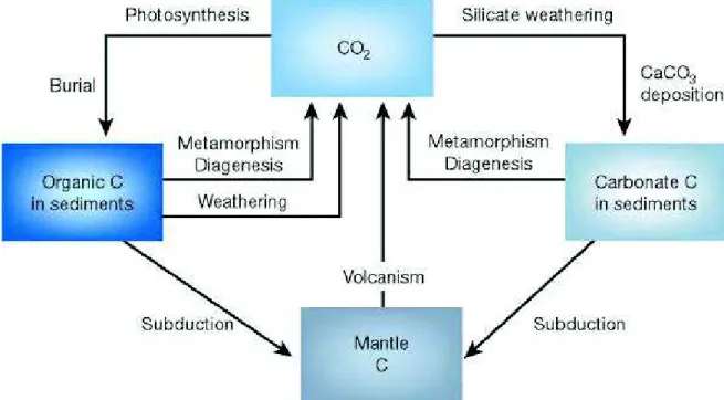
into solution will be transported across Earth’s surface by the rivers that eventually flow to the ocean. During this process, silicate weathering supplies cations (Caଶା and Mgଶା) to the oceans where they react with carbonate ions and precipitate Ca-Mg carbonate minerals. The weathering of silicate minerals followed by the deposition of carbonate minerals in the ocean to form carbonates and eventually sedimentary rocks is the main process by which carbon dioxide is transferred from the atmosphere back to solid earth (Figure 1-1) (Berner, 1992, 2003; Siever, 1968). The deep burial and thermal decomposition of carbonates releases carbon dioxide back into the atmosphere. After burial, carbon is recycled in the crustal material through plate subduction, where rocks under extreme temperature and pressure melt and recombine into silicate mineral. Finally, upon volcanic eruption, CO2is released back into the atmosphere where it can once again

bind with water molecules to form carbonic acid, react with silicate minerals when precipitated, and ultimately be consumed via silicate weathering (right side) or photosynthesis (left side), shown in Figure 1-1. In the case of photosynthesis uptake of CO2, carbon would be transferred to organic

material; upon death and burial, it will be transformed into organic carbon in sediments and eventually hydrocarbons. Oxidation or burning of organic matter / hydrocarbons releases CO2 to

(21)

the atmosphere, while deep burial and plate subduction returns carbon to the mantle where it is recycled (Berner, 2003).

Silicate weathering is governed by the rate of dissolution reactions which should depend mineralogy of the rocks and their characteristics (i.e. supply, exposed surface area, reactivity, etc.), availability of water and its residence time in the soil, soil pH, presence of vegetation (i.e. increasing production of organic acids and humic matter), and Arrhenius’ rate law which describes the temperature-dependency of the weathering reaction (Kump et al., 2000; Lasaga et al., 1994; Jackson, 1975). The temperature-dependence of this reaction on Earth’s surface

Figure 1-1. A model of the long-term carbon cycle. Source: Berner (2003).

has been proposed to provide the feedback mechanism that regulates climate over geologic timescales (Berner et al., 1983; Walker et al., 1981) and maintains relative climatic stability over Earth’s history. This hypothesis and other competing hypotheses regarding the chemical weathering – climate relationship will be further discussed in the next section (Section 1.2).

If temperature plays a crucial role in silicate weathering and thus promoting stable climatic conditions on Earth, being able to distinguish the role of the temperature from other factors that influence mineral dissolution reactions is vital. However, isolating the effect of temperature from other variables influencing chemical weathering such as precipitation, geomorphology, vegetation, and lithology has proven to be a difficult task (West et al., 2005).

(22)

There are two general approaches that are used to investigate the role of temperature on chemical weathering: laboratory experiments that focus on the mineral dissolution (rate-dependencies) as a function of temperature; and natural field experiments on various scales (individual rock types, soil profiles, and small and large catchments) typically measuring solute discharges. Field experiments are often used in combination with laboratory experiments to ground-truth laboratory results (Velbel, 1993a). Decades of laboratory experiments have focused on systematically defining the rate-dependency of silicate weathering reactions and mineral dissolution on these controlling factors, including temperature and solution chemical composition. The effects of temperature on the weathering rates of certain silicate minerals such as feldspars (Blum and Stillings, 1995), granites (White et al., 1999), quartz (Dove, 1995), and pyroxenes and amphiboles (Brantley and Chen, 1995) have been well established. These studies indicate that an increase in temperature from 0 – 25 C should increase weathering rates by approximately an order of magnitude (based on average experimental dissolution activation energies of 50 – 80 kJ/mol); an effect that is observable in natural environments. The activation energy is the energy that must be available for the chemical reaction to occur (Brady and Carroll, 1994). The effect of temperature on chemical weathering was also investigated both experimentally and in the field on fresh and weathered granitoid rocks, showing that increasing temperature correlates with an increase in Si dissolution, measured at four different sites (White et al., 1999) (Figure 1-2). Temperature trends for Si effluents are parallel for fresh and weathering paired granitoids, indicating that their sensitivity to temperature changes are similar regardless if they have experienced natural weathering. This implies that the nature of the weathering reactions are also similar. However, at any temperature, Si effluent concentrations from weathered rocks are lower than effluents taken from pristine rocks. White et al. (1999) also found similar relationships between the dissolution of Na and K in both fresh and weathered granitoids as a function of temperature (not shown). Additionally, a coupled temperature-precipitation model (White et al., 1999) produced apparent activation energies for Si which were comparable to those derived in the experimental field sites. This finding reinforces the fact that temperature significantly impacts natural silicate weathering rates. Several other studies have also shown the effects of temperature on the weathering and dissolution of various silicate minerals (e.g. anorthite, augite, kaolinite, smectite), demonstrating than in most cases an increase in temperature positively correlates with the rates of silicate mineral dissolution (e.g. Bauer and Berger, 1998; Brady and Carroll, 1994, among others). However,

(23)

silicate dissolution rates between laboratories are often inconsistent (within two orders of magnitude) and therefore generally considered to be not well-constrained (Brantley and Chen, 1995).

Figure 1-2. Arrhenius diagrams of the log Si effluent concentrations from both fresh and weathered granitoid rocks. The inverse of absolute temperature is displayed in the lower x-axis and the nonlinear scale to the temperature increase ( C) on the upper x-axis. Solid and dashed lines both correspond to linear fits of the effluent measurements of fresh and weathered granitoid rocks. Source: White et al. (1999).

Long term, direct observations in natural systems is the alternative approach to derive mineral weathering rates. Although this approach is a more direct way to study the relationship between temperature and weathering, it proves to be difficult because chemical, biological, and physical conditions, i.e. mineral compositions, temperature, surface area, fluid residence times and pathways, are generally not well-constrained. In addition, the time scale on which natural

(24)

weathering occurs is rarely able to be duplicated in experimental studies, accounting for and possibly explaining contradictions in silicate weathering rates among studies (White and Hochella, 1992). In general, as the scale in which we study weathering processes increases, our ability to detect and isolate a temperature signal decreases. This is mainly due to the complexity of interacting factors in larger systems and may explain why the comparison of solute concentrations and fluxes in the world’s largest rivers systems often fail to detect a temperature effect that is independent from other factors (Huh et al., 1998; Edmond et al., 1995). However, there have been a relatively small number of studies that have successfully isolated the effects of temperature from other factors. For example, estimated elevation-dependent temperature differences on the weathering of plagioclase minerals was determined in the Coweeta watershed (North Carolina) with a calculated activation energy of 77 kJ mol-1_{by Velbel (1993b) while Dorn and Brady (1995)}

used plagioclase porosity in Hawaiian basaltic flows sampled at different temperatures/elevations to calculate an activation energy of 109 kJ mol-1. In contrast, the study of weathering as function of temperature on the smaller scale has proved to be more rewarding. A compilation of works illustrating the impact of mean annual air temperature on weathering rates from various small granitoid catchments worldwide has been compiled by White and Brantley (1995) which collectively point to increased temperature and precipitation as a means to explain rapid weathering rates in various geographical settings (White et al., 1999). These efforts have significantly assisted weathering and kinetic models, for example, by providing rate constants for the dissolution of primary minerals (Brantley and Olsen, 2013; Hilley et al., 2010; White and Brantley, 1995). The positive correlations between dissolution rates of various minerals and rocks as a function of temperature both in the field and laboratory have provided support for the linkage between climate and silicate weathering on Earth’s surface.

Lithology is considered to be a major control on chemical denudation and weathering rates by controlling the composition of minerals involved in water-rock interactions and their susceptibility to weathering (Bluth and Kump, 1994; Meybeck, 1987; Peters, 1982; Garrels and Mackenzie, 1971). For example, mafic silicates in basalts such as olivine and pyroxene tend to be more reactive and weather much faster than felsic minerals in granites like quartz and feldspar. Meybeck (1987) reported a relative index of chemical weathering rates for common continental rocks ranging from 1–80: granites and gneisses being the lowest (1 - least likely to weather); limestones (12 – low to

(25)

intermediate) and saltrocks (80 - easier to weathering). This is because different minerals are composed of different elemental compounds which have different degrees of solubility in water. Generally, field studies that have sought to estimate the supply of major ions coming from specific lithologies often have had difficulties because the mobility of elements is dependent upon the parent rock composition (mineral composition, grain size, joints/fractures) and not geochemical processes alone (Sayyed, 2014). This problem became apparent in early studies that investigated the controls of stream chemistry at the watershed scale, i.e. (Peters, 1982; Garrels and Mackenzie, 1971), who found that the rates of dissolution and dissolved load chemistry are directly related to catchment lithology and the permeability of soils and bedrock material. The study of dissolved load chemistry at the basin scale, such as the Amazon, was undertaken by Stallard and Edmond (1983). The objective of this study was to determine the relationship between the major dissolved species in Amazonian rivers and factors such geology, topography, and the role of catchment soils. Results from this study also revealed that substrate catchment lithology and associated erosional regime were the major controls on the chemistry of surface waters within a catchment. For example, rivers that drained siliceous lithologies were relatively high in silica content and low in total dissolved cations; rivers draining carbonates were found to be high in alkalinity and intermediate levels of total cations. These results are consistent with mineral susceptibility trends for minerals in tropical environments such as the Amazon. More recent studies focusing on determining the global weathering rates and budgets by analyzing the dissolved load and suspended loads in large river systems (i.e. Bluth and Kump, 1994b; Gaillardet et al., 1999a) also report the dominant control lithology has on stream chemistry. Gaillardet et al. (1999a) reports that the chemical weathering (and possibly climate) signals carried by the rivers was also found to be dependent on and obscured by effects from parent lithology. The observation of the dependency of silicate weathering rates and intensities on parent lithology is not unique to studies focusing on large catchments nor to studies only using major and trace element as proxies for chemical weathering. For example, the chemical and isotopic compositions of dissolved load and solid phases carried by the river in small catchments may also be affected. A recent study of detrital material in stream sediments points to the strong control lithology has on the lithium (Li) isotopic composition of the clay fraction and therefore correct for it by subtracting the composition of bedrock from that of the sediment clay fraction before making any chemical weathering interpretations (Dellinger et al., 2017). Due to the inherent problem lithology often causes when

(26)

trying to get estimates of silicate weathering rates and access to the weathering regime in the field, many find it preferable to perform laboratory experiments on specific minerals (e.g. illites or smectites) (Williams et al. 2001a), or rock types such as basalts or granites (e.g. White and Brantley, 1995) and field experiments in small watersheds where monolithological units can be identified and studied (e.g. Dessert et al., 2003; Meybeck, 1987; Nesbit and Wilson, 1992).

The contributions of cations provided to streams and rivers by silicate weathering is to a large extent influenced by watershed hydrology and surface runoff and ultimately control the total dissolved yield in rivers (Garrels and Mackenzie, 1971). Additionally, the rates at which silicate weathering occur are thought to be a function of hydrology (Lasaga et al., 1994; Berner, 1978). Generally, the dissolution of minerals in water-saturated rocks, soils, and sediments are expected to rise with increasing flushing/flow rates up to a certain threshold where increased flow rates have no effect on dissolution (Berner, 1978); beyond the threshold, weathering reactions are no longer transport-controlled and become surface reaction-controlled. Therefore, one could expect weathering to be transport-limited at low flushing rates and surface-reaction controlled, also referred to as interface-limited, at high flushing rates. Holland (1978) reported TDS data from rivers worldwide as a function of runoff (Figure 1-3) which show that increasing flushing rates above a critical value do not increase the dissolve solid concentration in rivers throughout the world, but rather dilute them; a theory that is in agreement with Berner (1978). According to Schnoor (1990), lower flushing rates of field systems can account for the lower Si release rates observed in natural systems. Although this is the first order relationship between total dissolved solids (TDS) concentrations and runoff, other hydrological factors may also take part in this relationship to a lesser degree such as the activation of alternative flow ways and increasing drainage area during large storm events (Burns et al., 2001).

1.2 Chemical weathering and climate

Our current understanding of Earth’s climate system from Quaternary geology, including sedimentary, isotopic, and glaciological records, is that the climate system appears to be extremely sensitive to perturbations, particularly near critical thresholds between glacial and interglacial conditions (e.g. Rasmussen et al., 2014; Clement and Peterson, 2008; Ganopolski and Rahmstorf, 2001) . However, on longer time scales (millions to billions of years), we find a climate system

(27)

that is relatively stable and resilient to external forcing (Kasting, 1993). This would indicate that the processes affecting climate on shorter, millennial time scales may be components of positive feedbacks (where an initial change in the climate system leads to a secondary change which in turn enhances or magnifies the initial change) and those affecting climate on longer geologic time scales most often create negative feedbacks (where an initial change in the climate system leads to a secondary change which acts to reverse that initial

Figure 1-3. Total dissolved solids vs. runoff for rivers worldwide. The solid curve shows the general trend between TDS and annual runoff; solid line shows the dilution trend. The red dot shows the average values for the rivers worldwide. This figure demonstrates that past a critical threshold, increased runoff dilutes rather than increases TDS. Source: Holland (1978).

change) (Kump et al., 2000). Through positive feedbacks, subtle changes within the climate system can be detected and amplified (e.g. Curry et al., 1995), while the long-term response of the climate system acts within stable bounds through negative feedbacks (Walker et al., 1981). In the following, the current state of knowledge regarding potential drivers of chemical weathering and its relation to climate variability over both millennial and geologic timescales will be discussed.

(28)

1.2.1 Chemical weathering over geological timescales

Using the stratigraphic record, we can roughly estimate climatic conditions on Earth’s surface for the last 2.4 billion years, with more coherent estimates over the last 700 million years (Hambrey and Harland, 1981). Over the last 570 million years, four major glaciation events are recognized: Late Precambrian (1st_{); Ordovician-Silurian boundary (2}nd_{); Permo-Carboniferous}

(3rd); and, the present Cenozoic Era (4th) (Harland, 1981). The first, third, and fourth events are spaced roughly 300 million years apart and occur during times of continually low sea level (Vail et al., 1977). In contrast, the time period between the 1st and 3rd glaciations (Early- and Mid-Paleozoic), including the 2ndglaciation, corresponds to a general period of high sea levels and is similar climatically to the Mesozoic. Prior to Phanerozoic glaciations, there are several approximately known intervals of glaciation in the Proterozoic, with the oldest being in the Early Proterozoic (2.5 – 2.1 Ga ago) and several intervals in the Middle to Late Proterozoic (1.0 – 0.57 Ga) (Christie-Blick, 1982).

Significant climatic oscillations between greenhouse and icehouse states indicate that the mechanism(s) responsible for climatic regulation on Earth’s surface is (are) not perfect. However, they are able to correct for large climatic variations, thus promoting climatic stability over geological timescales and have not allowed the Earth to become locked into an inescapable Snowball Earth state (Caldeira and Kasting, 1992). Although some of the original energy-balance climate models such as those by Budyko (1969) and Sellers (1969) have predicted that a slight (2-5%) decrease in solar output could lead to a runaway glaciation, we now know that solar fluxes were 25-30% lower than present (Gough, 1981; Sagan and Mullen, 1972) and did not lead to irreversible freezing on Earth’s surface. Hence, the stability of Earth’s climate therefore requires a negative feedback between chemical weathering and climate and a mechanism allowing the extent of regulation or strength of the feedback to vary (Ruddiman, 1997).

Principle components of climate, i.e. temperature and precipitation, have been proposed to be responsible for controlling the rates of surficial silicate weathering and balancing the rates of atmospheric CO2production, thereby producing stable climatic conditions on Earth (Broecker and

Sanyal, 1998; Berner and Berner, 1997; Walker et al., 1981). Walker et al. (1981) suggested that the partial pressure of carbon dioxide in the atmosphere is buffered by a negative feedback

(29)

mechanism where the rate of weathering of silicate minerals, and subsequent deposition of carbonate minerals, is controlled by surface temperature, and surface temperature, in turn, depends on the carbon dioxide partial pressure via the greenhouse effect. If this hypothesis is correct, a link must exist between climate and tectonics in which a balance must be reached between planetary degassing of CO2 and the supply of CaO derived from the chemical weathering of

silicates. In theory, if the supply of CaO to the oceans were too small to match the input of CO2to

the ocean-atmosphere system, then the CO2 content of the atmosphere would rise, thereby

increasing the rate of chemical weathering until the system was balanced. On the contrary, if the rate of CaO supplied to the oceans were larger than the amount of CO2 inputted to the

ocean-atmosphere system, then the ocean-atmosphere’s CO2content would be drawn down causing the planet

to cool and thereby reducing the rate of chemical weathering. Although the quantitative estimates of this mechanism were crude, they were considered reasonable in partially explaining the stabilization of Earth’s surface temperature against the continuous increase in solar luminosity. Several subsequent studies (e.g. Broecker and Sanyal, 1998; Berner and Caldeira, 1997; Berner and Kothavala, 1994; Lasaga et al., 1985; Berner et al., 1983) have agreed with the hypothesis proposed by Walker et al. (1981).

For example, Berner et al. (1983) reconstructed the CO2 content of the atmosphere over

the last 100 Myr using a series of assumptions based on carbon cycling and geologic processes. Model outputs indicate that the CO2 content of the atmosphere is highly sensitive to changes in

rates of seafloor spreading and continental land area. Accordingly, this study reports that plate tectonics may have a major control on world climate. By calculating the changes in the carbonate chemistry of the modern surface ocean as function of varying amounts of CaO and calcite, Broecker and Sanyal (1998) conclude that the most likely mechanism to “police” or stabilize Earth’s climate is the CO2content of the atmosphere because it controls silicate weathering rates.

Berner and Caldeira (1997) found through a series of carbon mass balance equations that in the absence of a negative feedback mechanism, atmospheric CO2 levels would highly fluctuate.

Important conclusions were drawn from this study that support the now-accepted “Walker hypothesis”:

– Carbon inputs and outputs to and from the oceans, atmosphere, and biosphere are closely balanced over geological time scales

(30)

balance

– Silicate weathering response to climatic variability is sufficient to provide this negative feedback

– The rate of CO2 supply to the surficial system along with imbalances in the organic

carbon cycle control long-term global weathering rates

However, the CO2policing mechanism proposed by Walker et al. (1981) and agreed on by

others (e.g. Berner and Kothavala, 1994; Lasaga et al., 2013) did not go unchallenged by the scientific community. Raymo et al. (1988) and Raymo and Ruddiman (1992) were the first to challenge this concept which lead to a significant amount of controversy regarding the role of chemical weathering in regulating the atmospheric partial pressure of CO2, thus the extent and

strength of the greenhouse effect and global climate (Kump et al., 2000). Arguments in the literature generally center around the sensitivity of chemical weathering to various climatic factors, particularly temperature and to a lesser extent precipitation. Those that do not accept the climate-continental silicate weathering-atmospheric CO2relationship proposed by Walker et al. (1981) not

only question the effect of surface temperature on chemical weathering, but also point to other drivers of long-term control on atmospheric CO2such as tectonic uplift, denudation, and erosion

(Raymo et al., 1988), a combination of both tectonic uplift and climate (West et al., 2005), and global climate change (Molnar and England, 1990). Most notably, the hypothesis first proposed by Raymo et al. (1988) is likely the strongest opponent of the “Walker hypothesis” and is the center of controversy in the literature because it fundamentally challenges the idea that the Earth’s “thermostat” is controlled by balancing the rates of CO2 production via silicate weathering and

carbonate deposition which is ultimately a function of climate. The challenging “Raymo hypothesis” proposes that episodes of orogenic activity, i.e. tectonic uplift and erosion, may have caused increases in chemical weathering rates which resulted in a decrease of atmospheric CO2

concentration over the last 40 million years (Myr). This argument stems from the suggestion that the rapid uplift of the Himalayan-Tibetan plateau region and the Andes in the late Cenozoic had a significant impact on atmospheric circulation (Ruddiman et al., 1988). Using ocean box models of the geochemical cycles of strontium (Sr), calcium (Ca), and carbon (C) in marine sediments, Raymo et al. (1988) showed that the their record of carbonate sedimentation, calcite compensation depth,Ɂ଼଻Sr, and ɁଵଷC indicate increasing fluxes of weathering products to the sea over the past 5

(31)

Myr. It is proposed that this increase in chemical weathering rates over that time period caused a drawdown of atmospheric CO2 and therefore may have caused global cooling. By pairing their

marine record data with evidence of substantial mountain building throughout the world, enhanced uplift rates, and an apparent increase in global erosion, Raymo et al. (1988) conclude that chemical weathering rates and dissolved fluxes to the sea would increase stating the following reasons:

– rapid mechanical breakdown of rocks in areas experiencing rapid uplift would enhance exposure of primary minerals to chemical weathering, while abrasion of mountain stream would remove the iron-oxide coating that inhibits and slows weathering reactions (Stallard and Edmond, 1983)

– dissolved load of rivers are highest in areas that drain easily-eroded sedimentary rocks, a characteristic that is found in highly tectonic areas (Stallard and Edmond, 1983)

– Chemical and physical weathering rates increase with runoff which is often highest in mountainous regions because of the orographic effects of mountain ranges on precipitation patterns

The hypothesis that rapid uplift of the Himalayas and Tibet has the potential to change Earth’s atmosphere and climate over the Cenozoic period, proposed by Raymo et al. (1988), Raymo and Ruddiman (1992), and Ruddiman (1997), has found support of subsequent studies such as Hilley et al. (2010); and Hilley and Porder (2008). In an effort to shed light on how tectonics, climate, and rock-type influence silicate weathering and drive global rates, Hilley and Porder (2008) developed a model that considers whether local erosion rates, GCM-derived dust fluxes, temperature, and water balance can adequately capture global variation in silicate weathering. The model predicts that 50% of the atmospheric CO2 drawdown via silicate

weathering occurs in active mountain belts worldwide (20% within the Indo-Asian mountains) which lend support to the hypothesis that the continual uplift of the Himalayas over the late Cenozoic played a major role in regulating climate proposed by Raymo and Ruddiman (1992).

Hilley et al. (2010) then attempts to clarify the relative role that mineral supply and reaction may play on a select group of various mineral phases by modeling denudation and reaction kinetics. Laboratory and field measurement values of silicate weathering kinetic constants, observed weathering zone thicknesses, and denudation rates inferred from topography, were used

(32)

in the model. The study concludes that fresh mineral supply plays a dominant role in moderation silicate weathering fluxes for the minerals considered which suggests that the concentration of atmospheric CO2, which is regulated by silicate weathering over geological timescales, may

depend on those factors that control long-term erosion rates.

Another competing hypothesis to Walker et al. (1981) and Raymo et al. (1988) which essentially stems from the “Raymo hypothesis” is that proposed by Molnar and England (1990). In this case, the recent uplift of most mountain ranges documented by increased denudation and sedimentation rates, along with paleo-botanical evidence suggesting a shift to colder climatic conditions, are proposed to be the result of late Cenozoic climate change

In essence, they support the finding that erosion is controlled by climate (Wilson, 1973; Fournier, 1960), i.e. sediment yield is directly related to precipitation, and propose that increasing precipitation rapidly enhances erosion which causes isostatic rebound and uplift of the landscape. However, they argue that the mean elevation of the Himalayas perhaps did not rapidly accelerate over the Cenozoic, when accounting for both erosion and isostatic compensation of the landscape but that climate change, weathering, erosion, and isostatic rebound might interact in a system of positive feedback causing further global cooling. A more recent study (Willenbring and von Blanckenburg, 2010) has provided evidence of long-term stability of global weathering and erosion rates over the Cenozoic which partly contradicts the hypothesis proposed by Molnar and England (1990). Using the ocean dissolved 10Be/9Be record as a proxy for chemical weathering, stable weathering fluxes are observed over the past 12 Myr. Results from this study question whether the apparent fourfold increase in global sedimentation rates (driven by increased precipitation) proposed by studies such as Hay et al.(1988) has actually occurred. These results agree with other studies (e.g. Derry and France-Lanord, 1996) which suggest that an increase in burial of young organic matter (which would accompany increased sedimentation) is not apparent. Accordingly, the conclusions from this work are that neither global erosion nor weathering have increased as a results of climate change over the timescale of analyses (4 Mya) in spite of pulses of mountain building.

(33)

Over the last 420 ka, we observe four distinct glacial-interglacial sequences (Petit et al., 1999) (Figure 1-4); interglacial periods are characterized by a thicker greenhouse atmosphere (higher atmospheric CO2 and CH4 content), higher atmospheric temperatures, greater June

insolation (at 65 N), and more positive Ɂଵ଼O values in the atmosphere; during glacial periods we observe the opposite. The pattern of climate variability observed in the ice core can be described as ‘sawtooth’ during warm inter-glacial periods (stages 11.3, 9.3, 7.5 and 5.5), followed by increasingly colder interstadial events which end with a rapid return towards the following interglacial period (Petit et al., 1999). The coldest part of each glacial cycle occurs immediately before glacial termination and return to interglacial conditions, except in the third glacial cycle (225,000 to 325,000 yr BP), which according to Petit et al. (1999) may reflect a greater influence from the June 65 N insolation minimum prior to the transition. The ice core record presented by Petit et al. (1999), and others from Antarctica (Augustin et al., 2004) and Greenland (Andersen et al., 2004), have shown that the climate of the Earth over short timescales is sensitive to perturbations while oscillating within a stable bound between glacial and interglacial conditions.

Over 60 years have passed since the discovery of glacial-interglacial cycles via Ɂଵ଼O measurements in carbonates (Emiliani, 1955) and nearly 20 years since they have been thoroughly investigated using ice cores. Nevertheless, our current understanding of how silicate weathering has or will respond to climatic variability remains limited. This is primarily because until very recent times, the role of chemical weathering was thought to be slowly reactive to climate change and therefore only considered in studies investigating geologic climate variability (e.g. Livingstone, 1972). However, recent modeling efforts (Beaulieu et al., 2012) have shown that the weathering regime can respond very quickly (<100 yr) to changes in climate and may regulate atmospheric CO2 levels over short time periods. Although the role of climate on chemical

weathering is still debated, several studies (Bastian et al., 2017; Dosseto et al., 2015; Gislason et al., 2009) have challenged the notion that chemical weathering responds slowly to climate change and have shown that climate (temperature and precipitation) does play a role in determining chemical weathering regimes over