HAL Id: hal-01865236
https://hal.archives-ouvertes.fr/hal-01865236
Submitted on 31 Aug 2018
HAL is a multi-disciplinary open access
archive for the deposit and dissemination of
sci-entific research documents, whether they are
pub-lished or not. The documents may come from
teaching and research institutions in France or
abroad, or from public or private research centers.
L’archive ouverte pluridisciplinaire HAL, est
destinée au dépôt et à la diffusion de documents
scientifiques de niveau recherche, publiés ou non,
émanant des établissements d’enseignement et de
recherche français ou étrangers, des laboratoires
publics ou privés.
Attitude estimation from polarimetric cameras
Mojdeh Rastgoo, Cédric Demonceaux, Ralph Seulin, Olivier Morel
To cite this version:
Mojdeh Rastgoo, Cédric Demonceaux, Ralph Seulin, Olivier Morel. Attitude estimation from
polari-metric cameras. IEEE/RSJ Int. Conf. on Intelligent Robots and Systems - IROS, Oct 2018, Madrid,
Spain. �hal-01865236�
Attitude estimation from polarimetric cameras
Mojdeh Rastgoo
1, Cedric Demonceaux
1, Ralph Seulin
1, Olivier Morel
1Abstract— In the robotic field, navigation and path planning applications benefit from a wide range of visual systems (e.g. perspective cameras, depth cameras, catadioptric cameras, etc.). In outdoor conditions, these systems capture information in which sky regions cover a major segment of the images acquired. However, sky regions are discarded and are not considered as visual cue in vision applications. In this paper, we propose to estimate attitude of Unmanned Aerial Vehicle (UAV) from sky information using a polarimetric camera. The-oretically, we provide a framework estimating the attitude from the skylight polarized patterns. We showcase this formulation on both simulated and real-word data sets which proved the benefit of using polarimetric sensors along with other visual sensors in robotic applications.
I. INTRODUCTION
Large-field cameras and lenses (e.g. omnidirectional and fisheye cameras) are popular in robotic applications due to their ability to provide large field of view (up to 360◦), extending the amount of visual information. It is the main reason for which they have been adopted for a broad range of tasks such as visual odometry [25], navigation [31], simultaneous localization and mapping (SLAM) [14], and tracking [15]. With those systems, sky regions in the images acquired represent a large segment of information which are usually discarded. Here, we show that polarimetric informa-tion can be extracted from those regions and used in robotic applications.
Sun position, stars and sky patterns are hold as naviga-tional cues for the past centuries. Indeed, before the discov-ery of magnetic compass, these natural cues have been the solitary source of navigation used by our ancestors [2, 11]. Similarly, some insects used the skylight polarized pattern created by the scattered sunlight to navigate in their en-vironment [30, 16]. For instance, desert ants (cataglyphis), butterflies and dragonflies among others, are able to navigate through their paths, efficiently and robustly by using the polarized pattern of sky, despite their small brains [16, 30, 9]. Acknowledging the nature, numerous studies have been conducted on polarized skylight pattern [17, 4, 32, 29, 3, 1, 27, 19, 21, 28, 18, 9]. These studies are generally reported in the optic field. They focus on estimating the solar azimuth angle by creating a sort of compass. Estimating polarized patterns have been, however, a difficult and complex task. The primary studies report the use of several photodi-odes [17, 4, 32, 29, 3], or of multiple cameras [1, 27, 28] or manually rotating filters [19, 21, 18, 9]. As a consequence of those troublesome setups, robotic applications are not benefiting from the advantages of polarized patterns, as
1 Universit´e de Bourgogne Franche-Comt´e, Le2i VIBOT ERL-CNRS
6000, France,[email protected]
Fig. 1. Structure of DoFP sensors: in a single shot, four polarized images are acquired, each of them with a different polarized angles.
attested by the lack of polarized sensors used in Unmanned Aerial Vehicle (UAV). However, the recent introduction of division-of-focal-plane (DoFP) micropolarizer cameras has offered an alternative solution [23, 22, 20]. In such cam-eras a micropolarizer filter array, composed of a pixelated polarized filters oriented at different angles, is aligned with a detector array. Thus, linear polarization information are simultaneously acquired taking a single image. Here, we use a DoFP coupled with a fisheye lens to exploit the polarized information of sky region to estimate vehicle attitude.
In this paper, Sect. II presents the specificity of the camera used and the adaptation required for our robotic applica-tion. The remainder of the paper is organized as follows: Sect. III introduces the concepts of polarization by scattering, Rayleigh model and its relation with attitude estimation. Our formulation to estimate attitude is presented in Sect. IV. Experiments and implementation details are given in Sect. V, and finally discussions and conclusions are drawn in Sect. VI.
II. SETTING THE POLARIMETRIC CAMERA FOR ROBOTICS
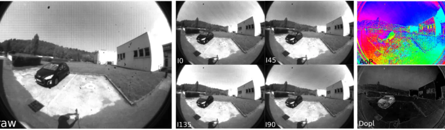
In this work, visual information is captured using the IMPREX Bobcat GEV polarimetric camera which is a DoFP polarimetric camera. In a single shot, the camera captures four different linearly polarized measures by using a mi-cropolarizer with pixelated polarized filter array as illustrated in Fig. 1. Hence, each acquired image is subdivided into four linearly polarized imagesI0,I45,I135, andI90. Subse-quently, the polarized state of the incident light is computed from these images by means of the Stokes’ parameters [8], referred ass0,s1, ands2in Eq. (1). In addition, the polarized parameters angle of polarization (AoP) and degree of linear polarization (DoPl), respectively referredα and ρlin Eq. (1) are computed.
Fig. 2. Polarimetric images: left: a raw images in which the different polarimetric images are interlaced; center: the four extracted linearly polarized images (I0, I45, I135, I90); right: the AoP and DoPl images. For visualization purpose, AoP is represented in HSV colorspace.
s0= I0+I45+I135+I90 4 , s1=I0− I90 , s2=I45− I135 , α = 0.5 arctan(s2 s1 ), ρl= ps2 2+s 2 1 s0 . (1)
The camera captures images with a resolution of 640 px × 460 px and each polarized image is reconstructed from the interlaced pixels. In addition, we used a 180◦ fisheye lens for the experiment reported in this paper to benefit from a large field-of-view. An example of an acquired raw image, the extracted polarized images and the computed polarized information is shown in Fig. 2
The IMPREX Bobcat GEV camera is controlled using the eBus SDK provided by Pleora Technologies Inc [5]. To enable the interaction with other robotic devices, we implemented a ROS package publicly available1 enabling the usage of roslaunch and rosrun. In addition, our package allows to store and stream the raw data as well as computing the Stokes’ and polarized parameters.
III. POLARIZED CUES USED FOR ATTITUDE ESTIMATION
Polarized cues used for attitude estimation are based on three main concepts which are presented in this section: (i) the Rayleigh scattering model and its implications on the polarization by scattering, (ii) the polarization parameters in pixel frame and its relation to camera, and (iii) the connection between the polarized parameters in the pixel frame and the parameters used to estimate the vehicle attitude.
A. Rayleigh scattering model
The unpolarized sunlight passing through our atmosphere gets scattered by different particles within the atmosphere. Besides deviating the direction of a propagated wave, this transition also changes the polarization state of the incident
1https://github.com/I2Cvb/pleora_polarcam. This
pack-age is derived from earlier work [12].
light which can be explained using the Rayleigh scattering model. Rayleigh scattering describes the scattering of light (or any electromagnetic waves) by particles much smaller than their transmission wavelength. Accordingly, it assumes that scattering particles of the atmosphere are homogeneous and smaller than the wavelength of the sunlight. Despite these assumptions, this model proved to be sufficient for de-scribing skylight scattering and polarization patterns [24, 10]. The Rayleigh model predicts that the unpolarized sunlight becomes linearly polarized after being scattered by the atmo-sphere. Based on this model, two main outcomes are drawn. On the one hand, DoPl is directly linked to the scattering angleγ according to:
ρl=ρlmax
1 − cos2(γ)
1 + cos2(γ) , (2) whereρlmaxis a constant equal to 1 in theory but slightly less
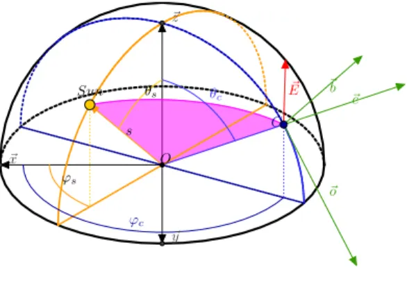
than 1 in practice due to some atmospheric disturbances [24]. The scattering angle γ is defined by the angle between the observed celestial vector~c and the sun vector ~s as presented in Fig. 3. Note that DoPl is 0 in the sun direction and maximum when the scattering angle is π2 [26, 21].
On the other hand, the scattered light is considered to be polarized and orthogonal to the scattering plane. Conse-quently, the Angle of Polarization is directly related to the orientation of the scattering plane.
B. Polarization by scattering model in pixel frame
As presented Fig. 4, an image is considered as a collection of pixels and each pixel measures the polarization parameters of the light traveling along a ray associated with that pixel. The pixel frame P is defined accordingly with the ray which coincides with ~c. The camera calibration determines the relationship between pixels and these 3D rays.
Let consider one pixel of the image with its associated pixel frame P ( cobc). Based on Rayleigh scattering, the elec-tric field of incident light after scattering is perpendicular to the scattering plane that is defined by the observer, celestial point, and the sun. Accordingly, the normalized electric field vector ~E in the world frame is presented as the normalized cross product of~s and ~c as shown in Eq. (3).
O Sun C ~ E ~b ~o ~c ~x ϕc ϕs ~y ~z θs θc s
Fig. 3. Skylight polarization by scattering. Scattering plane is highlighted by light shade of red. (θs, φs) and (θc, φc) define the zenith and azimuth
angle of sun and celestial point respectively. cobc defines the pixel frame, P, and ~E is the electrical field orthogonal to the scattering plane.
C Rcp xc yc zc ~ o ~b θc φc ~c P image plane
Fig. 4. Rotation between the camera frame C and one pixel of the frame P. The light ray associated to the pixels are represented in dark orange. The pixel that corresponds to the center of the image has obiously the same frame as the camera.
~
E = ~s ∧ ~c
k~s ∧ ~ck , (3) The same measurement in the pixel frame P is represented as: Eobc= Eo Eb 0 = cosα sinα 0 , (4)
whereα is the measured AoP associated to the corresponding pixel. Combining Eq. (3) & (4) and using the scattering angle γ, between ~s and ~c lead to:
(
(s ∧ c) · o = sin γ cos α
(s ∧ c) · b = sinγ sin α . (5) Applying the vector triplet cross product rule on Eq. (5) results in:
(
s · b = sinγ cos α
s · o = − sin γ sin α . (6) Using Eq. (2), the scattering angle γ is expressed as:
cosγ = s · c = ± s 1 −ρ0 l 1 +ρ0 l , (7) withρ0 l= ρlmaxρl .
Equations (6) & (7) finally lead to a representation of the sun vector in pixel frame P which express a direct relation between the AoP, the scattering angle, and the sun position:
~sp= − sin γ sin α sinγ cos α cosγ . (8)
In other words, the sun vector is expressed in the pixel frame as a vector depending only on the polarization parameters AoP and DoPl, which is directly linked to the scattering angleγ.
C. UAV attitude and polarized sky pattern
Figure 5 illustrates all transformations and frame con-ventions to estimate the attitude of a UAV. In addition, an inertial measurement unit (IMU) frame is added for later comparisons. W{EN U } V{F LU } I{RLD} C{RDF } Rww0 Rwv Rvi Rvc W0 Rw0i
Fig. 5. Frame conventions and rotations for attitude estimation of an UAV.
In Fig. 5, W, W0, I, V, C, and P refer to the world frame, global frame of IMU, IMU frame, vehicle frame, camera frame, and pixel frame, respectively. The rotation from one frame to another is presented with lowercase alphabet. In this scenario, a vectorvp in pixel frame is expressed in the world framevw as:
vw=Rwv· Rvc· Rcp· vp , (9)
where the rotation from the camera to the pixel frameRcp is obtained by camera calibration. The rotation is defined as the yaw and pitch rotations by the zenith and azimuth angles of the celestial point (θc, φc) as shown in Eq. (10).
Rcp=
cosθccosφc − sin φc sinθccosφc cosθcsinφc cosφc sinθcsinφc
− sin θc 0 cosθc , =Rzc(φc) ·Ryc(θc).
(10)
In Eq. (8), we expressed the sun position in the pixel frame. Indeed, this representation can be applied to any point from the world frame, ergo:
sw=Rwv· Rvc· Rcp· − sin γ sin α sinγ cos α cosγ , =Rwv· Rvc· v , (11) thus RT · sw=v . (12) The above equation shows a direct relation between the rotation matrix of the vehicle R, the AoP α — measured by the polarimetric camera at one pixel — and the angle of scattering γ for the corresponding pixel. In addition, if ρlmax is known, the angle of scattering is directly obtained by inverting Eq. (7) providing a direct relation between polarization parameters and the rotation of the vehicle.
IV. ATTITUDE ESTIMATION
In this section, we present 2 approaches to estimate the attitude: (i) in the former method named absolute rotation, the absolute rotation and attitude of the vehicle is estimated under the assumption that the sun position is known or deduced from time and the GPS location of the vehicle and (ii) in the latter method named relative rotation, the relative rotation of the vehicle from its initial position is estimated without additional assumption regarding the sun position. Both approaches required an estimate of the scattering an-gleγ which will be presented beforehand.
A. γ estimation
By only measuring the AoPα in scattering effects, γ needs to be estimated to get the vectorv defined in Eq. (11). This equation is valid for all points in sky region. However, only 2 celestial points are required to estimateγ such as:
Rt· s = R cp1· − sin γ1sinα1 sinγ1cosα1 cosγ1 Rt· s = R cp2· − sin γ2sinα2 sinγ2cosα2 cosγ2 . (13)
Using the product of Rcp and Rz(α), Eq. (13) is rewritten as: M1· 0 sinγ1 cosγ1 =M2· 0 sinγ2 cosγ2 . (14)
By defining the matrixM such that M = Mt
2· M1,γ1 and γ2 are found as:
(
γ1= − arctanMM0201 γ2= − arctanMM2010
. (15)
The AoP is 2π modulus, while the γ found in Eq. (15) is π modulus leading to two possible solutions for the vector v: (α1, γ1) and (α1+π, −γ1).
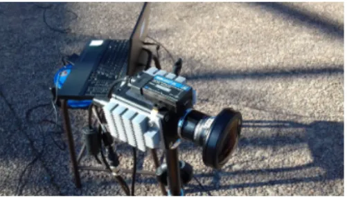
Fig. 6. Experimental setup.
B. Absolute rotation
In order to estimate the absolute rotation and attitude of the UAV, it is assumed that: (i) the sun position is known (ii) the vectorv is estimated using the AoP measures of the sky (2 points) and (iii) the vertical in the pixel frame is known or a second w is estimated using the AoP from horizontal reflected areas. In this study, the vertical in the pixel frame is assumed to be known.
The aforementioned assumptions lead to the following expression: ( [s, z, s ∧ z] = R(t) · [v(t), w(t), v(t) ∧ w(t)] =Rwv(t) · Rvc· [v(t), w(t), v(t) ∧ w(t)] . (16) wherez is the vertical in world frame ([0, 0, 1]) and t is the time instance.
Solving Eq. (16) enables to getRwv(t). However, due to γ ambiguities, v and therefore Rwv have 2 solutions. At each iteration, the rotation Rwv selected is the one the closest from previous rotation, assuming that the motion between two frames is smoothed.
C. Relative rotation
The relative rotation is estimated between two time stamps (t1,t2). Letv(t1) andv(t2) referring tov1andv2to simplify the expression. Therefore, Eq. (16) becomes:
( [s, z, s ∧ z] =Rwv1· Rvc· [v1, w1, v1∧ w1] [s, z, s ∧ z] =Rwv2· Rvc· [v2, w2, v2∧ w2] . (17) Leading to: Rwv2=Rwv1· Rvc· [v1, w1, v1∧ w1] · [v2, w2, v2∧ w2] −1 · RTvc , (18)
Using the above equation, the relative rotation Rv1v2 is
equal to: Rv1v2 = Rvc· [v1, w1, v1∧ w1] · [v2, w2, v2∧ w2] −1 · Rt vc . (19) As previously explained, only 2 points are required to compute the scattering angle γ. In practice (see Sect. V), more points can be used which leads to a more robust estimate of the vehicle rotation.
(a) AoP (b) DoPl (c) AoP (d) DoPl
Fig. 7. AoP and DoPl images synthetically created. All images have been generated with sky region for yaw, pitch and roll angle of 1.8 rad, −0.2 rad and 0.1 rad, respectively. (a)-(b) No noise added, (c)-(d) Noise level of 0.1 added.
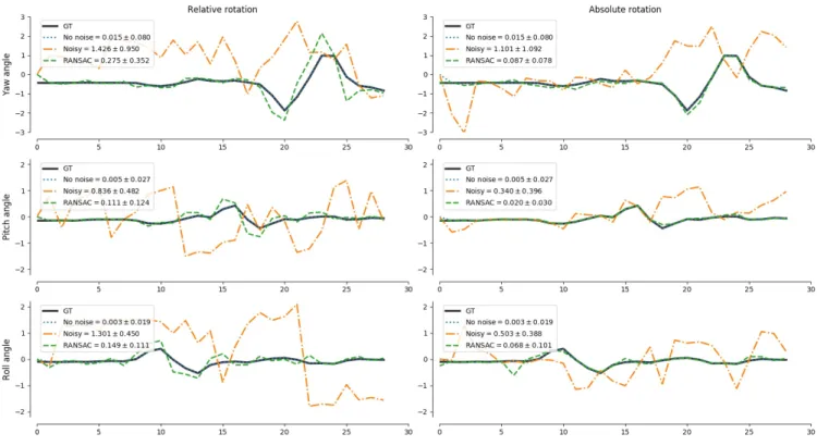
Fig. 8. Absolute and relative rotation obtained from synthetic data in ideal case, noisy conditions without RANSAC optimization and noisy case with RANSAC optimization. The mean and standard deviation of the difference between each predicted and GT is illustrated in the legend as well.
V. EXPERIMENTS ANDRESULTS
This section presents our experimental setup, the designed experiments and the obtained results. The setup used in our experiment is illustrated in Fig. 5. Instead of using a UAV, a camera was manually moved (see Fig. 6). The IMU was calibrated with the camera using kalibr toolbox [7, 6], to use the recordings as GT. The polarimetric camera with fisheye lens was also calibrated according to [13]. Using the above setup two data sets of synthetic and real images were created and the results obtained are presented in Exp. V-A and Exp. V-B, respectively.
A. Experiment 1
The synthetic data containing AoP and DoPl images of sky regions were created using the IMU recordings obtained during real acquisition. Figures 7(a) & 7(b) show an example
of this dataset at optimal conditions. This dataset based on IMU recordings contains rotations along roll, pitch, and yaw. This dataset has originally 856 samples but has been down-sampled by sampling rate of 30 samples.
Applying our framework on ideal synthetic data, perfect results were obtained for absolute and relative rotations, whileγ was estimated using only 2 random points from the sky region (blue dotted curve in Fig. 8).
Although using our proposed framework, we were able to achieve perfect results on ideal synthetic data, in reality it is rare to obtain the perfect skylight polarization pattern. Variety of causes clutter the desired skylight pattern, the main one being pollution. To account for such cases, a second test was performed while significant level of noise was added to the created synthetic data. Figures 7(c) & 7(d) show an example of synthetic data with an additional Gaussian noise with an
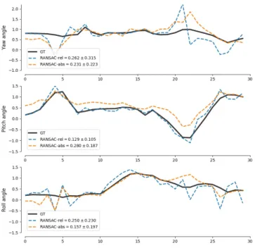
Fig. 9. Absolute and relative rotation obtained from real data. The black line represents the GT, the orange line and the blue line represent the absolute and relative predicted rotations, respectively.
standard-deviation of 0.1.
Performing the same 2 random-points algorithm as before on noisy dataset leads to the results illustrated in Fig. 8, the orange curve. As expected the performance decline, simply due to the noise.
To solve this problem, Random sample consensu (RANSAC) was used to estimate the attitude in the absolute and relative rotation methods. For the absolute rotation, since the sun position is assumed to be known the model optimizes the full rotation of each frame in comparison with the origin considering the difference between the predicted and real sun positions.
However, in the relative rotation method there is no infor-mation about the original position, or sun position, and the algorithm only depends on the polarized vector,v = Rcp.vp between two different frames. Therefore, using the model infers the optimal vector representing each frame is obtained. Estimating the attitude on the noisy dataset with RANSAC significantly improved the results as shown in Fig. 8 (green-dashed line). The parameters used were: an error threshold of 0.07, 10 random points (2 points for defining the model and the rest as test), and 2000 iterations.
The quantitative results in terms of mean difference (µ) and standard deviation (σ) between the predicted rotations and GT, for all the conditions are also shown in the Fig. 8. Note that all the angles are reported in radians.
As illustrated in the obtained results, using the RANSAC model the outliers are ignored and satisfactory results are achieved.
B. Experiment 2
This section presents the results obtained using real data. The same experimental setup was used using the IMU results to create the GT for the vehicle in the world frame. The original data set contains 593 recordings which was under-sampled to a sampling rate of 20 frames. Both absolute and relative methods were ran with RANSAC with the same parameters than in the previous experiment. The results are presented in Fig. 9.
Even though the difference between the predicted rotation and GT using the real data is higher than for the synthetic measurements the results are promising and the pose trajec-tory of the vehicle is respected.
VI. DISCUSSION ANDCONCLUSION
This paper presented a new method to estimate attitude of a vehicle using the polarization pattern of the sky. Contrary to conventional cameras, polarimetric cameras exploit part of images that represent the sky and we demonstrated how to take advantage of this property to estimate attitude. We first derived all equations that describe the relationship be-tween the rotation matrix of the vehicle and the polarization parameters. Herein, we proposed a model based on AoP measurements of the light beam scattered by the sky, subse-quently two approaches of the absolute attitude and relative attitude estimation were proposed. The former estimated the rotation the vehicle in comparison to the origin taking into account the sun position while the latter did not consider this assumption and estimated the position of the vehicle in the world frame considering two consecutive frames. Finally, in order to cope with the undesired artifacts and outliers that can occur during the measurements, a RANSAC model was integrated within our framework. Promising results were achieved after using RANSAC optimization, illustrating the potential and capacity of a polarimetric camera to be integrated in the robotic field. As future work, we will focus our attention to improve these preliminary results including a minimization process of the accumulated error of prediction using filtering. Aware that the polarimetric camera cannot be a standalone system for robust attitude estimation, we also plan to combine this modality with geometric information to improve the quality of the estimation.
VII. ACKNOWLEDGMENT
This work is part from a project entitled VIPeR (Polari-metric Vision Applied to Robotics Nav- igation) funded by the French National Research Agency ANR-15-CE22-0009-VIPeR.
REFERENCES
[1] J. R. Ashkanazy and J. Humbert, “Bio-inspired absolute heading sens-ing based on atmospheric scattersens-ing,” in AIAA Guidance, Navigation, and Control Conference, 2015, p. 0095.
[2] A. Barta, V. B. Meyer-Rochow, and G. Horv´ath, “Psychophysical study of the visual sun location in pictures of cloudy and twilight skies inspired by viking navigation,” JOSA A, vol. 22, no. 6, pp. 1023– 1034, 2005.
[3] J. Chahl and A. Mizutani, “Integration and flight test of a biomimetic heading sensor,” in Proc. SPIE, vol. 8686, 2013, p. 86860E.
[4] J. Chu, H. Wang, W. Chen, and R. Li, “Application of a novel polariza-tion sensor to mobile robot navigapolariza-tion,” in Internapolariza-tional Conference on Mechatronics and Automation. ICMA 2009. IEEE, 2009, pp. 3763–3768.
[5] eBus SDK, “eBUS SDK | Pleora Technologies Inc,” http://www. pleora.com/our-products/ebus-sdk, 2018.
[6] P. Furgale, T. D. Barfoot, and G. Sibley, “Continuous-time batch es-timation using temporal basis functions,” in Robotics and Automation (ICRA), 2012 IEEE International Conference on. IEEE, 2012, pp. 2088–2095.
[7] P. Furgale, J. Rehder, and R. Siegwart, “Unified temporal and spatial calibration for multi-sensor systems,” in Intelligent Robots and Systems (IROS), 2013 IEEE/RSJ International Conference on. IEEE, 2013, pp. 1280–1286.
[8] D. H. Goldstein, Polarized light. CRC press, 2017.
[9] M. Hamaoui, “Polarized skylight navigation,” Applied Optics, vol. 56, no. 3, pp. B37–B46, 2017.
[10] G. Horvath, A. Barta, J. Gal, B. Suhai, and O. Haiman, “Ground-based full-sky imaging polarimetry of rapidly changing skies and its use for polarimetric cloud detection,” Applied optics, no. 3, pp. 543– 559, 2002.
[11] G. Horv´ath, A. Barta, I. Pomozi, B. Suhai, R. Heged¨us, S. ˚Akesson, B. Meyer-Rochow, and R. Wehner, “On the trail of vikings with polarized skylight: experimental study of the atmospheric optical prerequisites allowing polarimetric navigation by viking seafarers,” Philosophical Transactions of the Royal Society of London B: Bio-logical Sciences, vol. 366, no. 1565, pp. 772–782, 2011.
[12] Iralab, “ROS device driver for PhotonFocus cameras based on Ple-oras eBUS Software Development Kit (SDK),” https://github.com/ iralabdisco/ira photonfocus driver, 2018.
[13] J. Kannala and S. S. Brandt, “A generic camera model and calibration method for conventional, wide-angle, and fish-eye lenses,” IEEE transactions on pattern analysis and machine intelligence, vol. 28, no. 8, pp. 1335–1340, 2006.
[14] J.-H. Kim and M. J. Chung, “Slam with omni-directional stereo vision sensor,” in International Conference on Intelligent Robots and Systems, 2003, vol. 1. IEEE, 2003, pp. 442–447.
[15] M. Kobilarov, G. Sukhatme, J. Hyams, and P. Batavia, “People tracking and following with mobile robot using an omnidirectional camera and a laser,” in IEEE International Conference on Robotics and Automation, ICRA. IEEE, 2006, pp. 557–562.
[16] T. Labhart and E. P. Meyer, “Neural mechanisms in insect navigation: polarization compass and odometer,” Current opinion in neurobiology, vol. 12, no. 6, pp. 707–714, 2002.
[17] D. Lambrinos, R. Mller, T. Labhart, R. Pfeifer, and R. Wehner, “A mobile robot employing insect strategies for navigation,” Robotics and Autonomous Systems, vol. 30, no. 12, pp. 39 – 64, 2000. [Online]. Available: http://www.sciencedirect.com/science/article/pii/ S0921889099000640
[18] H. Lu, K. Zhao, Z. You, and K. Huang, “Angle algorithm based on hough transform for imaging polarization navigation sensor,” Optics express, vol. 23, no. 6, pp. 7248–7262, 2015.
[19] T. Ma, X. Hu, L. Zhang, J. Lian, X. He, Y. Wang, and Z. Xian, “An evaluation of skylight polarization patterns for navigation,” Sensors, vol. 15, no. 3, pp. 5895–5913, 2015.
[20] J. Millerd, N. Brock, J. Hayes, M. North-Morris, B. Kimbrough, and J. Wyant, “Pixelated phase-mask dynamic interferometers,” Fringe 2005, pp. 640–647, 2006.
[21] D. Miyazaki, M. Ammar, R. Kawakami, and K. Ikeuchi, “Estimating sunlight polarization using fish-eye lens,” in IPSJ Transactions on Computer Vision and Applications, vol. 1, 2009, pp. 288–300. [22] G. P. Nordin, J. T. Meier, P. C. Deguzman, and M. W. Jones,
“Diffractive optical element for stokes vector measurement with a focal plane array,” in Proc. SPIE, vol. 3754, 1999, pp. 169–177.
[23] ——, “Micropolarizer array for infrared imaging polarimetry,” JOSA A, vol. 16, no. 5, pp. 1168–1174, 1999.
[24] I. Pomozi, G. Horvath, and R. Wehner, “How the clear-sky angle of po-larization pattern continues underneath clouds: full-sky measurements and implications for animal orientation,” The Journal of Experimental Biology, vol. 204, pp. 2933–2942, 2001.
[25] D. Scaramuzza and R. Siegwart, “Appearance-guided monocular om-nidirectional visual odometry for outdoor ground vehicles,” IEEE transactions on robotics, vol. 24, no. 5, pp. 1015–1026, 2008. [26] G. S. Smith, “The polarization of skylight: An example from nature,”
American Journal of Physics, vol. 75, no. 1, pp. 25–35, 2007. [27] W. St¨urzl and N. Carey, “A fisheye camera system for polarisation
detection on uavs,” in European Conference on Computer Vision. Springer, 2012, pp. 431–440.
[28] D. Wang, H. Liang, H. Zhu, and S. Zhang, “A bionic camera-based polarization navigation sensor,” Sensors, vol. 14, no. 7, pp. 13 006– 13 023, 2014.
[29] Y. Wang, J. Chu, R. Zhang, L. Wang, and Z. Wang, “A novel autonomous real-time position method based on polarized light and geomagnetic field,” Scientific reports, vol. 5, 2015.
[30] R. Wehner, “Desert ant navigation: how miniature brains solve com-plex tasks,” J Comp Physiol A, vol. 189, pp. 579–588, 2003. [31] N. Winters, J. Gaspar, G. Lacey, and J. Santos-Victor,
“Omni-directional vision for robot navigation,” in IEEE Workshop on Om-nidirectional Vision. IEEE, 2000, pp. 21–28.
[32] K. Zhao, J. Chu, T. Wang, and Q. Zhang, “A novel angle algorithm of polarization sensor for navigation,” IEEE Transactions on Instru-mentation and Measurement, vol. 58, no. 8, pp. 2791–2796, 2009.