Scalable and Interpretable Predictive Models for Electronic Health Records

HAL Id: hal-01877742

https://hal.inria.fr/hal-01877742

Submitted on 20 Sep 2018

HAL is a multi-disciplinary open access

archive for the deposit and dissemination of

sci-entific research documents, whether they are

pub-lished or not. The documents may come from

teaching and research institutions in France or

abroad, or from public or private research centers.

L’archive ouverte pluridisciplinaire HAL, est

destinée au dépôt et à la diffusion de documents

scientifiques de niveau recherche, publiés ou non,

émanant des établissements d’enseignement et de

recherche français ou étrangers, des laboratoires

publics ou privés.

Scalable and Interpretable Predictive Models for

Electronic Health Records

Amela Fejza, Pierre Genevès, Nabil Layaïda, Jean-Luc Bosson

To cite this version:

Amela Fejza, Pierre Genevès, Nabil Layaïda, Jean-Luc Bosson. Scalable and Interpretable Predictive

Models for Electronic Health Records. DSAA 2018 - 5th IEEE International Conference on Data

Science and Advanced Analytics, Oct 2018, Turin, Italy. pp.1-10. �hal-01877742�

Scalable and Interpretable Predictive Models for

Electronic Health Records

Amela Fejza

, Pierre Genevès

, Nabil Layaïda

, Jean-Luc Bosson

{amela.fejza, pierre.geneves, nabil.layaida}@inria.fr

†_{Univ. Grenoble Alpes, CNRS, Public Health department CHU Grenoble Alpes,} Grenoble INP, TIMC-IMAG, 38000 Grenoble, France

JLBosson@chu-grenoble.fr

Abstract—Early identification of patients at risk of developing complications during their hospital stay is currently one of the most challenging issues in healthcare. Complications include hospital-acquired infections, admissions to intensive care units, and in-hospital mortality. Being able to accurately predict the patients’ outcomes is a crucial prerequisite for tailoring the care that certain patients receive, if it is believed that they will do poorly without additional intervention. We consider the problem of complication risk prediction, such as inpatient mortality, from the electronic health records of the patients. We study the question of making predictions on the first day at the hospital, and of making updated mortality predictions day after day during the patient’s stay. We develop distributed models that are scalable and interpretable. Key insights include analysing diagnoses known at admission and drugs served, which evolve during the hospital stay. We leverage a distributed architecture to learn interpretable models from training datasets of gigantic size. We test our analyses with more than one million of patients from hundreds of hospitals, and report on the lessons learned from these experiments.

I. INTRODUCTION

One major expectation of data science in healthcare is the ability to leverage on digitized health information and computer systems to better apprehend and improve care. Over the past few years the adoption of electronic health records (EHRs) in hospitals has surged to an unprecedented level. In the USA for example, more than 84% of hospitals have adopted a basic EHR system, up from only 15% in 2010 [1], [12]. The availability of EHR data opens the way to the development of quantitative models for patients that can be used to predict health status, as well as to help prevent disease, adverse effects, and ultimately death.

We consider the problem of predicting important clinical outcomes such as inpatient mortality, based on EHR data. This raises many challenges including dealing with the very high number of potential predictor variables in EHRs. Traditional approaches have overcome this complexity by extracting only a very limited number of considered variables [5], [14]. These approaches basically trade predictive accuracy for simplicity and feasibility of model implementation. Other approaches have dealt with this complexity by developing black box This research was partially supported by the ANR project CLEAR (ANR-16-CE25-0010).

machine learning models that retain predictor variables from a large set of possible inputs, especially with deep learning [3], [18], [20], [22]. These approaches often trade some model interpretability for more predictive accuracy.

Predictive accuracy is crucial as wrong predictions might have critical consequences. False positives might overwhelm the hospital staff, and false negatives can miss to trigger important alarms, exposing patients to poor clinical outcomes. However, model interpretability is essential as it allows physi-cians to get better insights on the factors that influence the predictions, understand, edit and fix predictive models when needed [4]. The search for tradeoffs between predictive accuracy and model interpretability is challenging.

We consider complication risk prediction and focus on two aspects of this problem: (i) how to make accurate predictions with interpretable models; and (ii) how to take into account evolving clinical information during hospital stay. Our main contributions are the following:

• we show that with interpretable models it is possible to make accurate risk predictions, based on data concerning admitting diagnoses and drugs served on the first day. • we further develop mortality risk prediction models to

make updated predictions when new clinical information becomes available during hospitalization, in particular we analyze the evolution of drugs served.

• we report on lessons learned through practical experi-ments with real EHR data from more than one million of patients admitted to US hospitals, which is, to the best of our knowledge, one of the largest such experimental study conducted so far.

Outline: The rest of the paper is organized as follows: we first present the data and methods used in §II. In §IIIwe present results obtained when making predictions of clinical outcomes on the first day at the hospital. In §IVwe investigate to which extent the predictive models can benefit from the availability of supplemental information becoming available during the hospital stay to make updated predictions. We finally review related works in §Vbefore concluding in §VI.

II. METHODS A. Data source

We used EHR data from the Premier healthcare database which is one of the largest clinical databases in the United States, gathering information from millions of patients over a period of 12 months from 417 hospitals in the USA [19]. These hospitals are believed to be broadly representative of the United States hospital experience. The database contains hospital discharge files that are dated records of all billable items (including therapeutic and diagnostic procedures, med-ication, and laboratory usage) which are all linked to a given admission [15]. We focus on hospital admissions of adults hospitalized for at least 3 days, excluding elective admissions. The snapshot of the database used in our work comprises the EHR data of 1,271,733 hospital admissions.

B. Outcomes

For a given patient, we consider the problem of predicting the occurence of several important clinical outcomes:

• death: in-hospital mortality, defined as a discharge dispo-sition of “expired” [9], [20];

• hospital-acquired infections (HAI) developed during the stay [21];

• admissions to intensive care unit (ICU) on or after the second day, excluding direct admissions on the first day; • pressure ulcers (PU) developed during the stay (not

present at admission).

Patients who experienced a given outcome are considered positive cases for this outcome; those who did not are consid-ered negative cases. TableIpresents the distribution of patients with respect to the considered outcomes.

TABLE I: Number of instances for each case study. Problem studied Positive cases Negative cases Ratio

Mortality 28,236 857,005 3.29%

HAI 22,402 862,839 2.59%

ICU Admission 32,310 852,931 3.78%

Pressure Ulcers 23,742 861,499 2.75%

C. Preparing the data for supervised learning

Our methodology assumes no a priori clinical knowledge. For a given patient, we first extract a list E of elementary features including the age, gender, and admission type. Our models also use the list of admitting diagnoses known for a given patient as available in the EHR data at admission1_,

which we denote by A. Procedures can be performed during the hospital stay. We denote the list of procedures performed on the ith day of the stay (with i > 0) by Pi. We also consider the lists of drugs served, on a daily basis: Di denotes the list of drug names (and their quantities) served on the ith day.

1_{We use a list of unique identifiers encoded using The International}

Classification of Diseases, Ninth Revision, Clinical Modification known as ICD-9-CM.

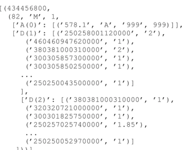
We filter out unused procedures and drugs, and use a perfect hash function to encode the features. The feature matrix is very sparse so in the implementation we use a sparse representation of feature vectors. Most patients are admitted at the hospital with at least one admitting diagnosis (among 5,094 possible diagnoses). A small proportion of patients receive procedures during their stay (∼ 20% of patients receive procedures on the first day). The total number of possible procedures is 11,338. Furthermore, during the stay, a total of 10,739 possible drugs can be served. On the first day of stay, a patient is served 8.6 drugs on average. Figure 1 shows the distribution of the considered population in terms of the number of drugs received on the first day. Figure 2 shows an excerpt of the data for a

0 20 40 60 80 100 Number of drugs 0 20000 40000 60000 80000 100000 Patients

Fig. 1: Population distribution in terms of the number of drugs received on the first day (|D1|).

sample patient. [(434456800, (82, ’M’, 1, [’A(0)’: [(’578.1’, ’A’, ’999’, 999)]], [’D(1)’: [(’250258001120000’, ’2’), (’460460947620000’, ’1’), (’380381000310000’, ’2’), (’300305857300000’, ’1’), (’300305850250000’, ’1’), ... (’250250043500000’, ’1’)] ], [’D(2)’: [(’380381000310000’, ’1’), (’320320721000000’, ’1’), (’300301825750000’, ’1’), (’250257025740000’, ’1.85’), ... (’250250052970000’, ’1’)] ]))]

Fig. 2: Data excerpt for a 82 years old male patient who went out alive on the third day.

D. Development of models

1) Interpretability: Following [4], we pay specific attention to the interpretability of the predictive models we develop. Model interpretability (or “intelligibility” as found in [4]) refers to the ability to understand, validate, edit, and trust

a learned model, which is particularly important in critical applications in healthcare such as the one we consider here. Accurate models such as deep neural nets and random forests are usually not interpretable, but more interpretable models such as logistic regression are usually less accurate. This often imposes a tradeoff between accuracy and interpretability. We choose to preserve interpretability and develop classifiers based on logistic regression. Advantages of logistic regres-sion include yielding insights on the factors that influence the predictions, such as an interpretable vector of weights associated to features, and predictions that can be interpreted as probabilities.

2) Mathematical formulation: Logistic regression can be formulated as the optimization problem min_w∈Rdf (w) in

which the objective function is of the form:

f (w) = λR(w) + 1 n n X i=1 θiL(w; xi, yi)

where n is the number of instances in the training set, and for 1 ≤ i ≤ n:

• w is the vector of weights we are looking for.

• the vectors xi ∈ Rd are the instances of the training data set: each vector xi is composed of the d values corresponding to features retained for a given admission. • yi ∈ {0, 1} are their corresponding labels, which we want to predict (e.g. for the mortality case study, 0 means the patient survived and 1 means the patient died at the hospital)

• R(w) is the regularizer that controls the complexity of the model. For the purpose of favoring simple models and avoiding overfitting, in the reported experiments we used R(w) = 1₂||w||2

2.

• λ is the regularization parameter that defines the trade-off between the two goals of minimizing the loss (i.e., training error) and minimizing model complexity (i.e., to avoid overfitting). In the reported experiments we used λ = 1

2.

• θi is the weight factor that we use to compensate for class imbalance. The classes we consider are heavily imbalanced (as shown in Table I): in-hospital death for instance can be considered as a rare event. Notice that we do not use downsampling (that would drastically reduce the set of negative instances for the purpose of rebalancing classes); instead we apply the weighting technique [13] that allows our models to learn from all instances of imbalanced training sets. θi is thus in charge of adjusting the impact of the error associated to each instance proportionally to class imbalance: θi= τ · yi+ (1 − τ ) · (1 − yi) where τ is the fraction of negative instances in the training set.

• the loss function L measures the error of the model on the training data set, we use the logistic loss:

L(w; xi, yi) = ln(1 + e(1−2yi)w

T_x i₎

Given a new instance x of the test data set, the model makes a prediction by applying the logistic function:

f (z) = 1 1 + e−z

where z = wTx. The raw output f (z) has a probabilistic in-terpretation: the probability that x is positive. In the sequel we rely on this probability to build further models (in particular using the stacking technique: see the meta-model built from such probabilities in §IV). We also use the common threshold t = 0.5 such that if f (z) > t, the outcome is predicted as positive (and negative otherwise)2_.

3) Scalability with distributed computations: a particularity of our study is that we want our models to be able to learn from very large amounts of training data (coming from many hospitals). We typically consider models for which both n and d are large: for instance n > 8 ∗ 105 _and d > 16 · 103 _{when we train models using features found in} EAD1. This is achieved by implementing a distributed version of logistic regression, including a distributed version of the L-BFGS optimization algorithm which we use to solve the aforementioned optimization problem. L-BFGS is known for often achieving faster convergence compared with other first-order optimization techniques [2]. We use a cluster composed of one driver machine and a set of worker machines3. Each worker machine receives a fraction of the training data set. The driver machine then triggers several rounds of distributed computations performed independently by worker machines, until convergence is reached. The software was implemented using the Python programming language and the Apache Spark machine learning library [17].

E. Model evaluation and statistical analysis

Patients were randomly split into disjoint train and test subsets. We perform k-fold cross validation with k = 5 unless indicated otherwise (k = 10 when indicated). Model accuracy is reported in terms of several metrics on the (naturally imbalanced) test set, which is used exclusively for evaluation purposes. We report on the receiver operator characteristic (ROC) curves and especially on the area under the ROC curve (AuROC). For the sake of completeness, we also include the commonly used Accuracy metric [8]. Since we deal with highly skewed datasets (as shown in TableI), we also report on the precision-recall (PR) curves and on the area under the PR curve (AuPR), in order to give a more complete picture of the performance of the models [6].

F. Prediction timing

We consider making predictions at different times. First, we consider making predictions on the first day at the hospital. We report on corresponding results, for all considered clinical

2_{We make t vary in [0, 1] for computing ROC curves.}

3_{Reported experiments were conducted with 5 machines (1 driver and 4}

workers), each equipped with two Intel Xeon CPU (1.90GHz-2.6Ghz), with 24 to 40 cores, 60-160 GB of RAM, and a 1GB ethernet network.

outcomes, in §III. We then report on how to make new mortal-ity predictions, day after day, whenever new EHR information becomes available, and present corresponding results in § IV.

III. RESULTS ONPREDICTIONS ON THEFIRSTDAY On the first day, we consider predictive models built with different sets of features (that we later combine). We name the models we consider after the sets of features they rely on. For example we consider the model EA for making predictions at hospital admission time t0 (i.e. at the moment when the patient arrives at the hospital). This model uses the elementary features E and the diagnoses A known at admission. We also consider making predictions whenever the set of drugs served on the first day is known (typically at t0+ 24h). For this purpose, we consider the model ED1 of [9] that uses elementary features and drugs served on the first day. All the considered models systematically use the elementary features E, so we often omit E in model names in the sequel. A. Mortality

For predicting in-hospital mortality, AuROC was 77.8% and AuPR was 12.7% with the D1 model, indicating significant predictive power of the drugs served on the first day (as already known from [9]). Over the total considered population of 1,271,733 patients, 885,241 (∼ 70%) of them have non-empty admitting diagnosis information at admission time (A6= ∅). AuROC was 76.4% and AuPR was 10.9% with the A model, which is aimed to leverage this information for making predictions directly at admission time. This indicates predictive power of the admitting diagnoses as well. It thus makes sense to study how these models could be combined to obtain more accurate predictions for the concerned population of 885,241 patients. We study combinations of the predictions made at admission with predictions made at t0+ 24h with the knowledge of the set of drugs served on the first day.

More generally, we consider different model combinations: • we consider models obtained by the flattening and con-catenation of features found in several basic models. In the sequel, we denote by C(B1, B2, ..., Bn) (or equiv-alently by B1B2...Bn) the single model obtained from the concatenation of the features used in the basic mod-els B1, B2, ..., Bn. For instance we consider the model C(A,D1) in which all the features found in A and D1 are concatenated.

• we also use ensemble techniques and in particular the stacking technique [7] to create combined models. The advantage of using logistic regressions as basic models to be combined with the stacking technique is that we can reuse not only their predictions, but also their raw output probabilities (which are more precise, as pointed out in § II-D2) as features for the meta-model. In the sequel, we denote by S(B1, B2, ..., Bn) the meta-model obtained from the raw probabilities of the basic models B1, B2, ..., Bn with the stacking technique. For example, we consider the model S(A,D1) built from the stacking of the two models A and D1.

Table II gives an overview of the AuROC, Accuracy and AuPR obtained with the basic and combined models con-sidered, on the same population, having admitting diagnosis information. Table II indicates the average, minimum and maximum values of each metric obtained with a 5-fold cross-validation process.

TABLE II: Mortality risk predictions on the first day.

Model AuROC % Accuracy % AuPR %

A 76.4 (76.0-76.8) 65.4 (65.2-65.6) 10.9 (10.6-11.2) D1[9] 77.4 (77.2-77.7) 74.5 (74.5-74.8) 12.3 (12.0-12.5)

S(A,D1) 80.1 (79.9-80.2) 69.2 (68.9-69.4) 14.0 (13.5-14.3)

C(A,D1) 80.4 (80.2-80.7) 75.3 (75.2-75.5) 14.2 (13.8-14.6)

We observe that the combined models yield significantly more accurate predictions than the basic ones, improving over comparable earlier works. For predicting inpatient mortality, with the AD1 model AuROC was 80.4% and AuPR was 14.2%, compared to respectively 77.4% and 12.3% obtained with the D1 model of [9].

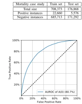
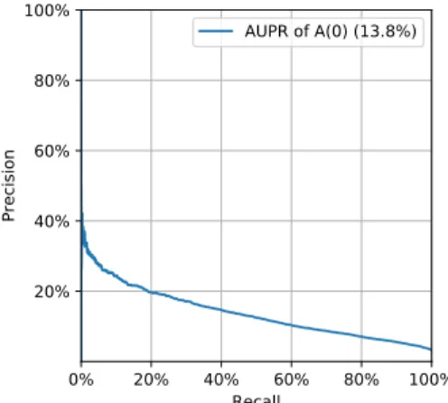
Figure3 presents the ROC curve obtained for a run of the C(A,D1) model on a given train and test set. The PR curve is shown on Figure 4. Table III presents sizes of train and test sets, and TableIVpresents the confusion matrix and associated metrics.

TABLE III: Number of instances for train and test sets. Mortality case study Train set Test set

Total size 708,373 176,868

Positive instances 22,660 5,576 Negative instances 685,713 171,292

0% 20% 40% 60% 80% 100%

False Positive Rate 20%

40% 60% 80% 100%

True Positive Rate

AUROC of A(0) (80.7%)

Fig. 3: ROC curve for mortality prediction at t0+ 24h.

B. HAI, ICU admission, and pressure ulcers

Table V presents results obtained when predicting all the other considered clinical outcomes using the C(A,D1) model. To the best of our knowledge, our models outperform state-of-the-art interpretable models found in the literature for

0% 20% 40% 60% 80% 100% Recall 20% 40% 60% 80% 100% Precision AUPR of A(0) (13.8%)

Fig. 4: PR curve for mortality prediction at t0+ 24h.

TABLE IV: Sample confusion matrix.

Actual Value Prediction outcome P0 _N0 _Total P 3,928 TP 1,648 FN 5,576 N 41,629 FP 129,663 TN 171,292 Total 45,557 131,311

TP is the number of true positives, FP the number of false positives, TN the number of true negatives and FN the number of false negatives.

True Positive Rate 70.4% (TP/(TP+FN) recall False Negative Rate 29.6% (FN/(TP+FN) miss rate

True Negative Rate 75.7% (TN/(FP+TN) specificity False Positive Rate 24.3% (FP/(FP+TN) fall-out Negative Predictive Value 98.7% (TN/(TN+FN)

Positive Predictive Value 8.6% (TP/(TP+FP) precision False Discovery Rate 91.4% (FP/(TP+FP)

Accuracy 75.5% (TP+TN)/(P+N) Error 24.5% (FP+FN)/(P+N)

TABLE V: Predictive accuracy on the first day.

Case study AuROC % Accuracy % AuPR %

Mortality 80.4 (80.2-80.7) 75.3 (75.2-75.5) 14.2 (13.8-14.6) HAI 84.8 (84.5-85.1) 84.2 (84.1-84.3) 20.6 (20.3-21.0) ICU 64.0 (63.7-64.3) 58.2 (58.1-58.5) 5.9 (5.7-6.0)

PU 82.2 (81.6-82.6) 78.3(78.2-78.5) 16.3 (16.0-16.5)

predicting hospital-acquired infections (AuROC was 84.8% vs 80.3% in [9]), and for predicting pressure ulcers (AuROC was 82.2% vs 80.9% in [9]). This suggests that classifiers trained from large amounts of diagnoses and drugs served found in EHR data can produce valid predictions across a variety of clinical outcomes (not only mortality) on the first day at the hospital.

C. Benefits of interpretability and explainability of predictions We investigate the stability and the consistency of the models when learned with different training sets. For this purpose, we study to which extent the logistic regression weights vary, when radically different training sets are ran-domly picked. In particular, we look for the most significant weights obtained from a run to another, ranking the weights in terms of their absolute values. For instance, we retained the 100 most important weights corresponding to A features (with the most significant absolute value) obtained for each random training set. We observe that the vast majority of the topmost weights remain the same accross each different run. A systematic pairwise comparison of the lists of topmost weights for each run showed that the least proportion of common weights between two runs was 90%.

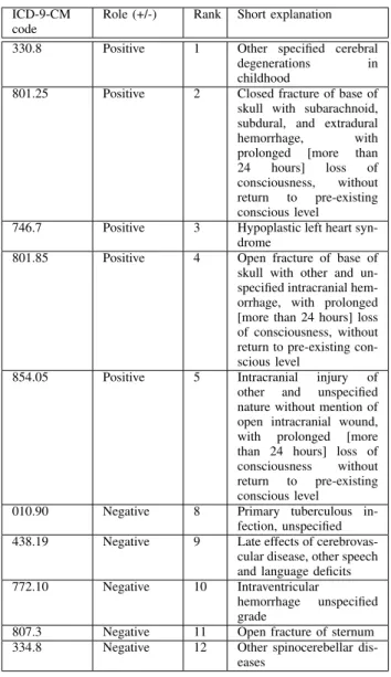
For example, Table VI presents an excerpt of the most important weights in the logistic regression model along with their ranking and their impact (positive/negative) on the out-come. Here “positive” is to be understood as a mathematically positive contribution in favor of the outcome (mortality). The clinical interpretation is beyond the scope of this paper, but the point is that our model allows this vector to be given to medical experts for further clinical research.

IV. RESULTS WITHEVOLVINGDATA

In this Section we study the problem of making mortality4

predictions no longer at hospital admission time but at a later stage during the hospital stay, while taking into account new clinical information becoming available since admission.

We consider making inpatient mortality predictions on a daily basis. We investigate interpretable models that predict on day k using data available up to that day. Therefore, in addition to elementary features (E), diagnoses (A) known at admission and drugs served on the first day (D1), we now consider the procedures Pidone on day i as well as the drugs Di served on day i, for i = 1 to k as bases for the predictions. A. Preliminary observations

Figure5gives insights on the number of patients remaining hospitalized at a certain day (no matter how long they stay). For each day i, it illustrates the subset of patients who have at least one drug served on that day (i.e. for which Di6= ∅), and the subset of patients who have a least one procedure on that day (i.e. for which Pi6= ∅) , respectively. The vast majority of

4_{Notice that the labeling of our data (for supervised learning) conveys the}

information of whether an ICU admission, HAI or PU occured during the hospital stay, but not exactly when it occurred. This is why in this Section we exclusively focus on predicting mortality when new data arrives (the date of death corresponding to the last date of the stay).

TABLE VI: Explanations of some ICD9-CM codes. ICD-9-CM

code

Role (+/-) Rank Short explanation

330.8 Positive 1 Other specified cerebral

degenerations in

childhood

801.25 Positive 2 Closed fracture of base of

skull with subarachnoid, subdural, and extradural

hemorrhage, with

prolonged [more than

24 hours] loss of

consciousness, without return to pre-existing conscious level

746.7 Positive 3 Hypoplastic left heart

syn-drome

801.85 Positive 4 Open fracture of base of

skull with other and un-specified intracranial hem-orrhage, with prolonged [more than 24 hours] loss of consciousness, without return to pre-existing con-scious level

854.05 Positive 5 Intracranial injury of

other and unspecified nature without mention of open intracranial wound, with prolonged [more than 24 hours] loss of consciousness without return to pre-existing conscious level

010.90 Negative 8 Primary tuberculous

in-fection, unspecified

438.19 Negative 9 Late effects of

cerebrovas-cular disease, other speech and language deficits

772.10 Negative 10 Intraventricular

hemorrhage unspecified grade

807.3 Negative 11 Open fracture of sternum

334.8 Negative 12 Other spinocerebellar

dis-eases

patients (more than 99.8%) are served drugs during their stay whereas only a small proportion of the population receive new procedures.

We first studied the evolution of procedures during hospital-ization. In particular, we created separate models using E and Pi as features for each day i; but their combinations with en-semble techniques did not yield any significant improvement in prediction accuracy over the global population5. One possible explanation for this is that the number of patients with Pi6= ∅ for i ≥ 1 remains too limited (as shown in Figure5). For this reason, we concentrate on the evolution of drugs served (Di for i ≥ 1) in the sequel.

5_{We did not obtain significant improvements when restricting to the patients}

having new procedures on the last day neither. Specifically, we filtered the population so as to retain only those patients who have at least one procedure at a certain day i. Since |Pi|=11,338, we conducted these analyses only until

day 2 (on which only 140,747 patients received procedures). AuROC obtained with P2was in the 69-70% range.

1 2 3 4 5 6 7 Day 0 200000 400000 600000 800000 Number of patients

Patients with non empty P(i) at day i Patients with non empty D(i) at day i

Fig. 5: Histogram illustrating the number of patients having at least one procedure or drug served on a given day.

B. Daily mortality predictions

For making predictions on a certain day k, we consider a variety of models built from different sets of features, that we combine with ensemble techniques (in a similar manner than for the first day – except that the set of basic models is now much richer as we can consider various models and several days). First, we consider all the models made with the features of one particular day [E,Di] for i = 1...k. We thus obtain k such models, each one composed of |E|+|Di| features. More generally, we also consider models in which we incorporate a sliding window of historical data available since admission by considering the features [EDk−w,Dk−w+1, ..., Dk] for w decreasing from k + 1 to 1. These models use up to n ∗ k+|E| features, where n is the number of possible drugs served (n = 10, 739). This can represent a very large number of features. To avoid running into the curse of dimensionality, we define a threshold for the maximum acceptable ratio between the number of features and the number of training instances (that decreases with higher values of k as shown in Figure5). We arbitrarily set this ratio to 10, which allows us to conduct analyses with sliding windows until the 6th _day.

For instance, Table VII presents the results obtained with all the basic models when predicting mortality on the 4th day of stay. First, we observe that AuROC, Accuracy and AuPR all raise when moving from a model Dk to a model Dk0 (for

1 ≤ k < k0≤ 4). This suggests that recent drugs served carry more accurate information on the current patient’s situation perspective of evolution. In particular, information on the last drugs served (Dk) improve the accuracy of predictions at day k. Models that do not leverage the latest drug information become less accurate with time, as shown in Table VII. Second, taking into account historical drugs served in the past few days (since admission) slightly improves AuROC and Accuracy.

This raises the question of how much historical data (since admission) it is worth to consider for making predictions (or in other terms, identifying tradeoffs between predictive

TABLE VII: Results for mortality prediction on day 4 (con-sidered population: patients that stay for at least 5 days).

Prediction Model features AuROC Accuracy AuPR

Day 4 D1 (72.5-73.1) (70.6-71.2) (11.5-12.3) Day 4 D2 (76.4-76.8) (74.6-74.9) (15.2-15.4) Day 4 D3 (78.3-79.2) (76.5-76.8) (18.0-18.5) Day 4 D4 (80.8-81.1) (78.8-79.1) (20.6-22.0) Day 4 D1D2 (76.8-77.0) (75.4-75.8) (15.1-15.6) Day 4 D1D2D3 (79.0-79.3) (77.7-78.1) (18.0-18.6) Day 4 D1D2D3D4 (81.1-81.5) (79.8-80.2) (21.0-21.5) Day 4 D2D3D4 (80.9-81.4) (79.3-79.7) (21.0-22.0) Day 4 D3D4 (80.8-81.4) (79.1-79.4) (21.0-22.0)

accuracy and model complexity). Table VIII presents the performance metrics obtained when predicting with models with different sizes of moving windows of historical data. Notice that the AuROC obtained with a model on day i is not directly comparable to the AuROC obtained for predictions at admission time in §IIIbecause they do not correspond to the same population (some patients left the hospital or died before day i). Each row of Table VIIIreports results for a different population filtered based on lengths of stay: predictions made at day i concern the population of patients that stayed for at least i + 1 days.

TABLE VIII: Predictive accuracy with different historical windows (min and max values obtained with 5-fold cross validation).

Day Model AuROC Accuracy AuPR

2 D2 (81.9-82.3) (79.1-79.5) (17.1-18.2) D1D2 (82.5-82.7) (79.9-80.1) (17.3-18.1) 3 D3 (81.0-81.7) (79.1-79.2) (18.9-21.0) D2D3 (81.4-82.0) (79.5-79.7) (19.4-20.7) D1D2D3 (81.6-82.3) (80.0-80.2) (19.3-20.7) 4 D4 (80.8-81.1) (78.8-79.1) (20.6-22.0) D3D4 (80.8-81.4) (79.1-79.4) (21.0-22.2) D2D3D4 (80.9-81.4) (79.3-79.7) (21.0-22.0) D1D2D3D4 (81.1-81.5) (79.8-80.2) (21.0-21.5) 5 D5 (80.8-81.0) (78.6-78.8) (23.0-23.4) D4D5 (80.7-81.2) (78.9-79.3) (22.7-23.7) D3D4D5 (80.5-81.2) (79.1-79.4) (22.5-23.7) D2D3D4D5 (80.3-81.1) (79.4-79.7) (22.0-23.6) D1D2D3D4D5 (80.4-81.2) (79.9-80.1) (22.5-23.8)

Results suggest that [Dk] models provide an interesting tradeoff (between accuracy and complexity) for predicting on day k compared to all the other models. One possible explanation for the limited accuracy improvements obtained with historical data since admission is that Dj carries most of the information from Dj−1 for any j. Figure 6 gives an overview of the (high) similarities between drugs served on consecutive days. We computed the number of common drugs served in two consecutive days for a given patient, which we normalize with respect to the total number of drugs served. The distribution of the population in terms of this ratio is shown in Figure 6a for the first two days, and in Figure 6bfor the next two days, respectively. We observe that for the majority of patients, the set of drugs served tend to only slightly change

from a day to another, a majority of drugs being continuously served day after day.

0.2 0.4 0.6 0.8 1.0

Fraction of common drugs 0 50000 100000 150000 200000 250000 Patients

(a) Between day 1 and day 2.

0.2 0.4 0.6 0.8 1.0

Fraction of common drugs 0 50000 100000 150000 200000 250000 300000 350000 400000 Patients

(b) Between day 2 and day 3.

Fig. 6: Similarities between drugs served on different days.

C. Discussion

All the predictions we made in this Section consider drug served data from the first day and onwards, but do not take into account the data A known as cause of admission (as opposed to § III). This means that the corresponding models can be directly used for making predictions for potential patients arriving at the hospital without available admitting diagnosis. For patients having an admitting diagnosis (∼ 70% of the overall population), we study combinations of the predictions made at admission (from § III) with predictions made later during the stay.

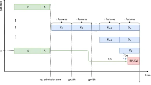
Figure7illustrates the different kinds of considered models. For instance, AuROC of the meta-model S(A,D1,D2,D3) was 82.2%. This suggests that data known at admission still helps in improving the accuracy of mortality predictions made at a later stage during the hospital stay. Table IX presents the

TABLE IX: Weights of meta-model S(A,D1,D2,D3).

Weights Model features 2.237623 probability using A 1.160006 probability using D1

1.292319 probability using D2

... ...

t0: admission time

n features n features n features

D1 D2 Dk-1 patients ... ... time t0+24h t0+48h f(z) f'(z) S(A,Dk) x A E Dk n features Dk-1 Dk Dk A E Predictions at day k ...

Fig. 7: The different kinds of models considered.

weights of the meta-model S(A,D1,D2,D3). We observe that the most important weight is associated with the A basic model. Then, the most important weights are associated, in decreasing order of importance, from the most recent to the oldest models. The higher influence on the final prediction thus comes from the admitting diagnoses, and then, from the drugs served in the most recent days.

So far, results suggest that when admitting diagnoses are available (A6= ∅), then they should be used as they increase the predictive accuracy. Otherwise (when A= ∅), relying on the last drugs served (Dk) provides a reasonable tradeoff for making mortality prediction at a certain day k > 0 of the stay. We now concentrate on studying how models with admitting diagnoses (A) can be combined with the models offering reasonable tradeoffs in terms of accuracy and complexity obtained so far (i.e. Dk). Each row of TableXreports results for a population filtered based on lengths of stay (predictions made at day i concern the population of patients that stayed for at least i + 1 days). We observe that the AuROC of the predictions made with A decreases over time with the remaining population (as also illustrated by the blue line in Figure 8). We also observe a (much slighter) decrease in AuROC when predicting with the latest drugs served. It is rather intuitive that predictions made only with data known at admission (A) become less accurate with time. This suggests that, due to changing conditions, we are progressively left with more complex cases (that stay longer at the hospital), whereas the population with imminent outcome progressively leaves day after day (either dead or alive).

Results show that the combined stacking model always outperforms the other basic models in terms of AuROC. After a certain period though, say on day k, models considering admitting diagnoses (A) start to be outdated enough so that predictions made only with this model progressively carry less useful additionnal predictive power to be leveraged by

the stacking. Therefore the net increase in predictive power brought by the S(A,Dk) model erodes with time. This starts to occur significantly for k ≥ 6, as illustrated on Table X and Figure8. In conclusion, the joint analysis of the evolution of drugs served with admitting diagnoses helps in improving the AuROC of predictions made at any moment during the hospital stay, especially for short stays.

TABLE X: Predictive accuracy with stacking models.

Prediction on Model AuROC Accuracy AuPR

Day 2 _DA (76.0-76.8) (65.2-65.6) (10.9-11.2) 2 (81.3-81.9) (79.2-79.3) (16.3-18.0) S(A,D2) (83.0-83.7) (73.5-74.0) (18.5-19.1) Day 3 _DA (73.8-74.1) (63.1-63.6) (10.4-11.1) 3 (80.6-81.4) (79.1-79.2) (18.6-19.9) S(A,D3) (81.9-82.5) (73.2-74.0) (19.8-20.7) Day 4 _DA (72.0-72.8) (61.0-61.8) (10.7-11.3) 4 (80.5-81.2) (78.8-79.2) (20.6-21.8) S(A,D4) (81.5-82.0) (72.9-73.2) (21.2-22.9) Day 5 _DA (70.0-71.7) (59.7-60.4) (11.3-11.7) 5 (80.1-81.1) (78.4-78.9) (21.5-24.2) S(A,D5) (80.6-81.1) (72.1-72.8) (22.4-23.3) Day 6 _DA (69.1-70.8) (58.3-58.8) (11.4-12.4) 6 (79.7-80.8) (77.9-78.4) (23.3-26.0) S(A,D6) (80.2-80.6) (71.6-72.2) (23.9-24.7) V. RELATEDWORKS

The interest in developing predictive systems for EHR data has soared recently. The automated identification of at-risk profiles is a topic that has been actively investigated under various forms, including: prediction of hospital length-of-stay, readmissions, discharge diagnostics, occurence of hospital-acquired infections, admissions to intensive care units, and in-hospital mortality. Several lines of work can be identified from the perspective of the methods used.

The first line of works gathers “score-based approaches”. These works build on decades of research by clinicians and

2.0 2.5 3.0 3.5 4.0 4.5 5.0 5.5 6.0

Day of prediction

AuROC

Fig. 8: Ranges of AuROCs obtained with A, Dkand S(A,Dk).

statisticians for attempting to measure the complexity of a patient’s situation according to a yardstick index. The basic idea boils down to computing an aggregate score or index from EHR data. For a given patient, the value of the index is meant to represent the severity of the patient’s condition and perspectives of evolution. Typical examples include the seminal Charlson comorbidity index [16], and the Medication Regimen Complexity Index (MRCI) [10]. The MRCI is a global score meant to indicate the complexity of a prescribed medication regimen. It aggregates 65 aspects related to the drug dosage form, dosing frequency and instructions. The greater the MRCI, the more complex the patient’s situation is. The minimum MRCI score is 2 (e.g. one tablet taken once a day) and there is no maximum. The main advan-tages of score-based approaches, besides their simplicity, are that scores are well-defined and commonly accepted among clinicians, easily implementable, computationally cheap, and understandable even by non-experts. However, if scores can give a rapid estimation of a general patient’s condition, their usage for predicting particular outcomes is still open. The work [14] shows positive correlations between the MRCI value at admission and the occurence of complications later during the hospital stay. It remains unclear though to which extent such correlations might actually be leveraged in a predictive system. More generally, score-based approaches suffer from significant drawbacks when it comes to building accurate predictive systems. Reducing a priori the whole patient’s situation and outcome to a single scalar value is questionable for two reasons. First, this aggregation is performed independently from any specific outcome to be predicted (like a particular complication). Second, many subtleties in EHR data (like drug interactions) are potentially discarded during the score computation. This may result in rough approximations. In the case of MRCI for instance, the same MRCI value may denote distinct situations with radically different perspectives of evolution.

A very recent line of work consists in analysing EHR data in a more comprehensive way, trying not to resort to a priori simplifications such as scores but trying instead to preserve as

much as possible of the original EHR information to analyse it in a fine-grained way. For instance, the works found in [3], [4], [9], [20] apply supervised machine learning techniques to a wide range of features selected from EHR data. These works can be subdivided into two further subcategories: (i) those that trade model interpretability for numeric accuracy and (ii) those which preserve model interpretability, usually at the price of some loss in accuracy.

Among the first category, we find the works [3], [20] that develop classifiers based on deep neural networks (DNNs). The models proposed in [20] typically achieve areas under the ROC curve within the 0.79-0.89 range for mortality prediction at admission on their dataset (they do not report on AuPR nor on accuracy though). It would be interesting to compare the complete picture of the predictive performances of the models proposed in [20] with the ones proposed in the present paper on the same dataset. Unfortunately [20] does not contain enough details on the features used in their models to allow for a reimplementation of their technique. Further comparisons with [20] are thus inappropriate because the datasets are different: they consider a lower number (216,221) of patients but with more data per patient (including historical data before admission, which we do not have in our dataset). In comparison, we analyse many more (1,271,733) patients with less data per patient (no history in particular). Notice that this makes our models more broadly applicable since they apply to patients for which we have no history at all.

It is also worth noticing that the results reported in [20] are achieved with an important sacrifice: a major drawback of DNNs is their lack of interpretability, as notoriously known. Preliminary works on explaining “black-box” models are rather in early stage [11]. Interpretability happens to be crucial for healthcare models so that they can be given to domain experts (e.g. clinicians) to be checked and fixed when necessary [4] using domain-expert medical knowledge. This is one reason why simple linear models (such as logistic regression) might be preferred over DNNs even when their accuracy is significantly lower, as detailed in [4].

Finally, the results described in [20] come at another price too: the computational cost. The computing power necessary for learning DNN classifiers with large amounts of data and large feature spaces is significant (an earlier version of [20] mentions more than 201,000 GPU hours of computation using Google Vizier for building the DNNs and setting up the hyper-parameters that crucially affect their performance). Compared to [20], our predictions are obtained with interpretable models, which yield interpretable weights (SeeIII-C) in particular. Our models are also lighter computationally and more scalable (one model is trained on 1.2 million of instances in around 4 minutes on a commodity cluster of 5 machines).

In the second category of works, we find [4] that advocates the use of the so-called “intelligible” models and apply them to two use cases in healthcare. The first use case is concerned with the prediction of pneumonia risk. The goal is to predict probability of death so that patients at high risk can be admitted to the hospital, while patients at low risk are treated

as outpatients. Their intelligible model provides an AUC in the 0.84-0.86 range, and uncovers patterns in the data that previously had prevented complex learned models from being fielded in this domain. The second use case is the prediction of hospital readmission, for which the developed model provides an AUC in the range 0.75-0.78. The datasets considered in [4] are uncomparable to the dataset we use in the present paper. For the prediction of pneumonia risk, [4] considers a dataset of 14,199 pneumonia patients with 46 features. For the prediction of hospital readmission, [4] considers 296,724 patients from a large hospital, with 3,956 features for each patient. Features include lab test results, summaries of doctor notes, and details of previous hospitalizations. Our problem formulation is different as we concentrate on predicting the risks of in-hospital mortality and other complications for any patient admitted to the hospital. We also consider a larger dataset (>1.2M patients) with more features, thanks to a distributed implementation.

The work found in [9] also applies linear models such as logistic regression for building binary classifiers. The goal is similar: making predictions of complications at hospital admission time. In § III we applied our method on the same dataset so the results can be directly compared. Our method provides significant improvements in accuracy: for mortality prediction our method achieves an AuROC in the range 80.2-80.7% (Accuracy: 75.3%) compared to 77.9% (Accuracy: 75%) reported in [9]. Similar improvements in accuracy can also be observed when predicting other complications (HAI, PU) considered in [9]. By leveraging admitting diagnoses (A), our method thus makes it possible to obtain even more accurate predictions when compared to [9]. The models proposed in [9] remain useful for patients with no admitting diagnosis. Finally and more importantly, compared to [9], we investigate the problem of making updated mortality predictions whenever more EHR data become available during the hospital stay (SectionIV), which is not considered in [9].

VI. CONCLUSION ANDPERSPECTIVES

We develop a distributed supervised machine learning sys-tem for predicting clinical outcomes based on EHR data. We propose interpretable models, based on the analysis of admitting diagnoses and drugs served during the hospital stay. Our models can be used to make predictions concerning the risk of hospital-acquired infections, pressure ulcers, and inpatient mortality. We study how mortality risk models can be extended with the analysis of the evolution of drugs served during the stay. We use a distributed implementation to train models on millions of patient profiles. We report on lessons learned with a large-scale experimental study with real data from US hospitals. One perspective for further work would be to study to which extent the system generalizes for predicting other clinical outcomes such as long lengths of stay and hospital readmissions.

REFERENCES

[1] J. Adler-Milstein, A. J. Holmgren, P. Kralovec, C. Worzala, T. Searcy, and V. Patel. Electronic health record adoption in u.s. hospitals: The

emergence of a digital ’advanced use’ divide. Journal of the American Medical Informatics Association, 24(6):1142–1148, Nov 2017.url. [2] G. Andrew and J. Gao. Scalable training of l1-regularized

log-linear models. In Machine Learning, Proceedings of the International Conference (ICML), pages 33–40, 2007.url.

[3] A. Avati, K. Jung, S. Harman, L. Downing, A. Y. Ng, and N. H. Shah. Improving palliative care with deep learning. In Proceedings of the IEEE International Conference on Bioinformatics and Biomedicine, pages 311–316, 11 2017. url.

[4] R. Caruana, Y. Lou, J. Gehrke, P. Koch, M. Sturm, and N. Elhadad. Intelligible models for healthcare: Predicting pneumonia risk and hos-pital 30-day readmission. In Proceedings of the 21th ACM SIGKDD International Conference on Knowledge Discovery and Data Mining, pages 1721–1730, August 2015. url.

[5] Y. Choi, C. Y.-I. Chiu, and D. Sontag. Learning low-dimensional representations of medical concepts. AMIA Summits on Translational Science Proceedings, 2016:41–50, 2016. url.

[6] J. Davis and M. Goadrich. The relationship between precision-recall and ROC curves. In Machine Learning, Proceedings of the International Conference (ICML), pages 233–240, June 2006.url.

[7] T. G. Dietterich. Ensemble methods in machine learning. In Intl workshop on multiple classifier systems, pages 1–15. Springer, 2000. [8] T. Fawcett. An introduction to ROC analysis. Pattern Recogn. Lett.,

27(8):861–874, jun 2006.url.

[9] P. Genevès, T. Calmant, N. Layaïda, M. Lepelley, S. Artemova, and J.-L. Bosson. Scalable machine learning for predicting at-risk profiles upon hospital admission. Big Data Research, (12):23–34, 2018. url. [10] J. George, Y. Phun, M. J. Bailey, D. C. Kong, and K. Stewart.

De-velopment and validation of the medication regimen complexity index. Annals of Pharmacotherapy, 38(9):1369–1376, 2004. url.

[11] R. Guidotti, A. Monreale, F. Turini, D. Pedreschi, and F. Giannotti. A survey of methods for explaining black box models. CoRR, abs/1802.01933, 2018. url.

[12] J. Henry, Y. Pylypchuk, T. Searcy, and V. Patel. Adoption of electronic health record systems among u.s. non-federal acute care hospitals: 2008-2015. url, may 2016.

[13] G. King and L. Zeng. Logistic regression in rare events data. Political Analysis, 9(2):137–163, 2001. url.

[14] M. Lepelley, C. Genty, A. Lecoanet, B. Allenet, P. Bedouch, M.-R. Mallaret, P. Gillois, and J.-L. Bosson. Electronic medication regimen complexity index at admission and complications during hospitalization in medical wards: a tool to improve quality of care? International Journal for Quality in Health Care, 2017. url.

[15] R. Makadia and P. B. Ryan. Transforming the premier perspec-tive®hospital database into the observational medical outcomes part-nership (omop) common data model. eGEMs, 2(1):1110, 2014.url. [16] C. ME, P. P, A. KL, and M. CR. A new method of classifying prognostic

comorbidity in longitudinal studies: development and validation. J Chronic Dis., 40(5):373–83, 1987. url.

[17] X. Meng, J. Bradley, B. Yavuz, E. Sparks, S. Venkataraman, D. Liu, J. Freeman, D. Tsai, M. Amde, S. Owen, D. Xin, R. Xin, M. Franklin, R. Zadeh, M. Zaharia, and A. Talwalkar. Mllib: Machine learning in Apache Spark. CoRR, abs/1505.06807, 2015. url.

[18] R. Miotto, L. Li, B. A. Kidd, and J. T. Dudley. Deep patient: An unsupervised representation to predict the future of patients from the electronic health records. Scientific Reports, 6, May 2016. url. [19] Premier. Healthcare database, Feb 2018. url.

[20] A. Rajkomar, E. Oren, K. Chen, A. M. Dai, N. Hajaj, M. Hardt, P. J. Liu, X. Liu, J. Marcus, M. Sun, P. Sundberg, H. Yee, K. Zhang, Y. Zhang, G. Flores, G. E. Duggan, J. Irvine, Q. Le, K. Litsch, A. Mossin, J. Tansuwan, D. Wang, J. Wexler, J. Wilson, D. Ludwig, S. L. Volchenboum, K. Chou, M. Pearson, S. Madabushi, N. H. Shah, A. J. Butte, M. D. Howell, C. Cui, G. S. Corrado, and J. Dean. Scalable and accurate deep learning with electronic health records. npj Digital Medicine, 1(1):18, 2018. url, An earlier version appeared in eprint arXiv:1801.07860.

[21] D. Roosan, M. Samore, M. Jones, Y. Livnat, and J. Clutter. Big-data based decision-support systems to improve clinicians’ cognition. In Proceedings of the IEEE International Conference on Healthcare Informatics, pages 285–288. IEEE, December 2016. url.

[22] B. Shickel, P. J. Tighe, A. Bihorac, and P. Rashidi. Deep ehr: A survey of recent advances in deep learning techniques for electronic health record (ehr) analysis. IEEE Journal of Biomedical and Health Informatics, 2017. url.