Click-based ultrasonic gesture recognition

(1)

1

Click-based Ultrasonic Gesture Recognition

by

Temitope (Tosin) Olabinjo

S.B. E.E.C.S., M.I.T., 2019

Submitted to the

Department of Electrical Engineering and Computer Science In Partial Fulfillment of the Requirements of the Degree of

Master of Engineering in Electrical Engineering and Computer Science

at the

Massachusetts Institute of Technology

May 2020

Signature of Author: ________________________________________________________ Department of Electrical Engineering and Computer Science

May 12, 2020

Certified by: ________________________________________________________

Dennis M. Freeman, Henry Ellis Warren Professor of Electrical Engineering Thesis Supervisor

Certified by: ________________________________________________________

Nathan Blagrove, Manager, Bose Applied Research Software Engineering Group VI-A Company Thesis Supervisor

Accepted by: ________________________________________________________

(2)

2

Click-based Ultrasonic Gesture Recognition

by

Temitope (Tosin) Olabinjo

Submitted to the Department of Electrical Engineering and Computer Science

on May 12, 2020 in Partial Fulfillment of the Requirements for the Degree of Master of Engineering in Electrical Engineering and Computer Science

Abstract

To maximize the potential of future human-computer interaction, advancements in the methods by which people interface with computers must be made. This study aims to establish the foundation for a new, contactless method of input powered by ultrasonic echolocation. The project consists of three main sub-studies; one short COMSOL study, and two rounds of data collection at different levels of detail. We built and analyzed COMSOL models in order to gain an initial sense of the feasibility of ultrasonic gesture recognition. The detailed data collection trials demonstrated a clear correlation between ultrasonic echoes and motion. During the rough data collection trials, we laid the groundwork for future endeavors which aim to use machine learning to build ultrasonic gesture recognition systems. Analysis of the data gained from the rough data collection trials made the preliminary conclusions of the detailed data collection trials more concrete.

M.I.T Thesis Supervisor: Dennis M. Freeman

Title: Henry Ellis Warren Professor of Electrical Engineering

VI-A Company Thesis Supervisor: Nathan Blagrove

(3)

3

List of Figures

Figure 1- COMSOL models of speaker (left) and hand (right) ... 11 Figure 2 - Frames from animation of an impulse from the speaker and the reflection off of the hand ... 12 Figure 3 - Graphs of the sound pressure level measured at a point near the speaker ... 13 Figure 4 - Detailed data collection workflow ... 15 Figure 5- Audacity screenshot featuring spectrograms of the reference signal (bottom) and the recordings from mic1 and mic2 (top). The ultrasonic clicks are visible in every channel. ... 16 Figure 6 - Images of a user wearing the OptiTrack head and hand markers; The headset (blurred) is on the couch but is worn during the trial. ... 17 Figure 7- Workflow for sample window extraction ... 22 Figure 8 - Example frames from click animation ... 23 Figure 9 - Example frames from click animation which overlays information from multiple audio sources... 24 Figure 10 - Motion data from Trial000, position (left) and velocity (right), graphed over the course of the entire trial ... 29 Figure 11 - Data from Trial000, zoomed-in to a single sequence of actions. ... 30 Figure 12 - Motion data from Trial001, position (left) and velocity (right), graphed over the course of the entire trial ... 30 Figure 13 - Data from Trial001, zoomed-in to a single sequence of actions (position – left , velocity – right) ... 30 Figure 14 - Comparison of Trial000’s motion graphs generated using different types of

timestamps, automatic (left) and manual (right). ... 32 Figure 15 - Comparison of the motion graphs generated using different types of timestamps, zoomed in to a small sequence of actions ... 32 Figure 16 - Key frames of the 'b' clicks from mic 1 during Trial001 ... 33 Figure 17 - The number of lobes in the reflected signal depends on the volume of the source audio. ... 34 Figure 18 - Screenshot of spectrograms of individual clicks. The window on left depicts clicks played at high volume, the one on the right features clicks played at a low volume ... 35 Figure 19 - Key frames of the ‘b’ clicks from mic 2 and reference signal ... 35 Figure 20 - Comparison of processed audio norm and norm-difference graphs ... 36 Figure 21 - Comparisons between processed audio data and OptiTrack motion data (position – Top, velocity – Bottom) ... 38 Figure 22 - Subset of position and audio data from Trial000, all values are scaled to be between 0 and 1 ... 40 Figure 23 - Subset of velocity and audio data from Trial000, all values are scaled to be between 0 and 1 ... 40 Figure 24 – Zoomed-in portion of graph which features overlaid position and audio data ... 41

(6)

6

Figure 25 - Setup for rough data collection featuing, the GUI, position markers, and headset (blurred out) ... 44 Figure 26 - Example of a position prompt from the rough data collection GUI ... 47 Figure 27 - Rough data collection workflow ... 50 Figure 28 - User inputting their ID at the beginning of a data collection session, the headset is on but obscured by the user's hair ... 51 Figure 29 -User holding their hand at the close (left) and middle (right) positions as dictated by the data collection script ... 51 Figure 30 - Average echoed click at each position for a single user ... 53 Figure 31 - Average echoed click at each position across multiple users ... 53 Figure 32 - Average echoed clicks at each position across multiple users, zoomed into click .... 54 Figure 33 - Spectrograms of average clicks at each position ... 55 Figure 34 - Spectrograms of average clicks at each position, zoomed into click ... 55 Figure 35 - Average norm-difference graph across multiple users for each position ... 56

(7)

7

1. Introduction

1.1 Vision

Touchscreens revolutionized how we interact with all forms of technology. Freeing software developers from the limits on input imposed by ten-digit numpads enabled them to invent innovative interactions between users and their phones. The aim of this project is to further expand the range of ways one can interact with technology. By employing ultrasonic sensing and signal processing, this project demonstrates the feasibility of ultrasonic gesture recognition systems. For this project I built a suite of tools which can be used in future endeavors which aim to combine machine learning and ultrasonic sensing to build a system which detects and identifies a user’s gestures. With an ultrasonic gesture recognition system, a user could control any device without having to touch any part of it, no buttons or screens necessary.

Ultrasonic sensing has been studied in the past. However, most efforts rely on specialized hardware built specifically for ultrasonic frequencies. Those studies speak to the potential of ultrasonic sensing, but the specialized hardware hinders the technology’s ability to be applied to consumer devices. My goal is to evaluate the efficacy of an ultrasonic sensing system composed of commonplace audio components.

1.2 Background Research

Multiple groups have approached ultrasonic sensing from various angles. Several of them investigate systems which use the technology to track and analyze human motion. In 2018, at Tsinghua University in Beijing, Yu Sang, Laixi Shi, and Yimin Liu developed a system which can detect and discern micro hand gestures using ultrasonic active sensing. Sang’s system employed several pieces of specialized ultrasonic hardware, namely a MA300D1-1 Murata

(8)

8

Ultrasonic Transceiver, to obtain extremely accurate information on the motion of one’s fingers, (Sang). While effective, this hardware cannot be found in most publicly available personal devices.

In 2016, Rajalakshmi Nandakumar, and her team of researchers from both the University of Washington and Microsoft Research, used the standard audio equipment on smart watches and cellphones to track finger motion. Nandakumar and her team achieved measurements with

accuracy down to 1cm using standard hardware. Their system employs long (5-6ms) Orthogonal Frequency division multiplexing (OFDM) signals to track finger motion. Nandakumar’s study focused on the displaying the robustness of their finger tracking system, demonstrating its ability to sense when it was occluded by a jacket sleeve or the fabric of a pocket, (Nandakumar).

Focused solely on motion tracking, their study did not explore any methods of gesture recognition, such as using machine learning to determine user intent.

1.3. Previous Work

Prior to my assignment at Bose Corporation in Framingham, MA, the groundwork for this project was laid through work that focused on building and testing the hardware which generates the ultrasonic tones. This work included preliminary investigations into whether the headsets available at Bose Corporation were capable of emitting and receiving ultrasonic frequencies. It was found that a selected headset was equipped with both i) speakers that could emit ultrasonic tones and ii) microphones that could pick up those tones with an acceptable signal-to-noise ratio.

The previous work at Bose Corporation drew heavy inspiration from the signals emitted by Egyptian fruit bats, leading to the decision to employ ultrasonic clicks instead of a continuous tone. Using ultrasonic clicks opens the door to various forms of analyses on the echoed clicks,

(9)

9

such as time-of-flight and analysis of the transformed click received by the microphones. The previous work at Bose Corporation also drew inspiration from the dolphins referenced by Dr. Timothy Leighton in his lecture, The Acoustic Bubble. In his lecture, Dr. Leighton explained how dolphins use a two-part signal to identify and differentiate between small objects in the water such as bubbles and fish. The dolphins’ two-part signal inspired the decision to make the signal for this project a series of pairs of clicks - one big, one small.

Lastly, in designing the clicks, a Gaussian waveform was chosen instead of a square wave in order to maximize the signal-to-noise ratio. Using a square wave introduced undesirable noise into the system.

2. Projected Contributions

My work goes beyond the contributions of previous efforts in a few key areas. First, the use of standard hardware, as opposed to specialized components, serves to further diminish the barriers between this technology and bringing it to market. Secondly, for this project we employ click-based sonar drawing inspiration from the method of echolocation used by Egyptian fruit bats. Egyptian fruit bats can discern targets with diameters as small as 5 cm by emitting

(ultrasonic) clicks and listening for the echoes (Yovel). Other studies that employ sonar generally use long signals and tones that are not like these short (~1 ms) bat-like clicks. In this study, we evaluate the accuracy of a click-based sonar system and compare its performance to non-click-based approaches. In developing our system, we also assess the efficacy of various forms of analysis to decode gesture information embedded in ultrasonic echoes. In order to manage the scope of this project, we are limiting our gesture data to inferences on the position and motion of

(10)

10

the entire hand. The gathering of information on the motion of individual fingers to is left to future iterations of this project.

Ultimately, this system lays the groundwork for a new, reliable method of interaction with personal devices. Future endeavors will be able to use the tools and data developed during this project to build machine learning models which will enable contactless control of various devices.

3. COMSOL Modelling

3.1 Overview

COMSOL is a fairly intricate multi-physics simulation software capable of modeling the effects of elements such as electricity, heat, gravity, etc. on various objects. Much of the

strength of COMSOL lies in the amount of freedom the software offers to the user to customize the details of their models and the parameters of the physics at play in their simulations.

Additionally, COMSOL’s extremely customizable environment allows for the creation of various different scenarios without reconfiguring any actual hardware.

For this project we use COMSOL to model ideal instances of what our system aims to accomplish. The hope is that COMSOL models of idealized versions of our system will provide a better understanding of the acoustic principles at play when we are actually building the system.

3.2 Design

Every COMSOL model we generated consists of a representation of a speaker and a microphone. The speaker is modelled by a point source, set to emit a pressure wave at an ultrasonic frequency of our choosing. The microphone is modelled by an acoustic pressure

(11)

11

measurement point. The microphone model doesn’t take up any physical space or bear any physical characteristics. Simplifying the microphone model enables us to move the microphone around, and take measurements from, different points within the simulation space fairly easily without introducing extra surfaces for the sound to bounce off of.

Figure 1- COMSOL models of speaker (left) and hand (right)

Some of our simulations also include a model of a hand. To model a hand, we use a flat disk with rounded off edges and major radius of several inches. In the center of one face of the disk we placed a cone-like indentation whose base is close in diameter to that of the disk. This indentation represents the concave nature of the average person’s hand.

One drawback of striving to create detailed COMSOL models is that, on hardware that is not equipped to handle large, detailed graphics simulations, the generation of the simulations can take an exorbitant amount of time. One of the more complex simulations I created took about three days to render. In order to cut down on processing time we designed our models with a focus on simplicity. Using a measurement point for the microphone and a point source for the speaker cut down on the number of elements which needed to be simulated. Making the hand radially symmetric allowed us to employ 2d axisymmetric models. 2d axisymmetric models are

(12)

12

essentially 2d models that are extruded radially around an axis. This way one can model a 3d system that capitalizes on the simplicity of a 2d system.

3.3 Results

The images below depict several frames of the animated simulation of a single click being emitted from a point source and later reflected by our simplified model of a hand.

Figure 2 - Frames from animation of an impulse from the speaker and the reflection off of the hand

The graphs below display measurements of the sound pressure level at a point near the sound source. This measurement is meant to mimic the signal received by the microphone over the course of a single click. This example serves to illustrate how a sound impulse can travel through air, be reflected by the surface of a hand (a rigid boundary in our model), and have its echo make it back to a spot near the source at an amplitude still strong enough to be measured. The two graphs were created from taking measurements during a click from different points in the space. The fact that the two graphs differ offers credence to the belief that information on location can be gained through an analysis of sound reflections.

(13)

13

Figure 3 - Graphs of the sound pressure level measured at a point near the speaker

3.4 Preliminary Conclusions

While this model does provide evidence to support the feasibility of our proposed set up in an extremely controlled setting, it does not paint a completely accurate picture of the sonic characteristics of the environment we will be testing in. In reality, our system will be operating in an environment with many more surfaces present. A user’s hair, objects in the office, passersby, even the structure of a user’s ear etc. can all act as surfaces for our signal to reflect off of. In order to better mimic the conditions we modeled in COMSOL, we will strive to limit

obstructions between the headset and the user’s hand during testing.

Due to the tremendous amount of time and computational effort required to sufficiently design, build, and render more accurate COMSOL models, and the very limited timescale of this project, we decided to move forward with the preliminary findings gleaned from COMSOL and go straight into live trials. Future investigators in this field may find value in continuing to develop more elaborate models in COMSOL. It appears to be a very powerful tool which can yield very useful results given sufficient time and computing power.

(14)

14

4. Detailed Data Collection

4.1 Overview

In order to gain a working knowledge of the correlations between motion and ultrasonic echoes we developed a system to gather and analyze detailed information on both motion and audio. The goal is to establish whether the data contained within ultrasonic echoes contains enough information to differentiate between various positions and motions of a hand. This information can later be used to determine what gestures are being performed. To gather detailed information on motion we use an OptiTrack system. OptiTrack is a system of motion capture capable of recording actions as small as the motion of a finger. Much of the motion-capture effects in The Lord of the Rings trilogy employed a similar system. To record high fidelity audio, we use Audacity, a commonly-used, open-source, audio recording and editing tool. Finally, I built several scripts to process, analyze, and display the data collected from these sources.

4.2 Design

Overview of Data Collection Workflow

The overall flow of detailed data collection proceeds as follows. To begin collecting detailed data the subject must put on the head and hand OptiTrack markers, making sure all other OptiTrack markers are out of sight with respect to the system’s cameras. The user must ensure that OptiTrack is set up to look for, and output information regarding, those two markers. After setting up OptiTrack, the user puts on the headset which should be plugged into the laptop that is being used for data collection. The laptop should have three programs pulled up, Audacity, an audio player with the desired clicking audio pulled up, and a terminal program set to run the OptiTrack data collection python script. The user starts the clicking audio by hitting play in the audio player. Then, possibly with some assistance, they should start the OptiTrack script and

(15)

15

Audacity recording at the approximately the exact same time. Once all the recoding has begun, the user performs various gestures, making sure to keep their hand in line with the headset. After completing the desired set of gestures, the user exits out of the OptiTrack script, and then stops and saves the Audacity recording.

This flow chart illustrates the workflow of a detailed data collection session.

Figure 4 - Detailed data collection workflow

Setup for Collecting Audio

Physical setup: To emit ultrasonic clicks we passed the audio through the speaker of the headset. To record audio, we use the microphones on the headset. The headset has two

microphones, one towards the front of the device and one towards the back.

Software Setup: In the beginning of the project, we used a Jupyter notebook developed at Bose Corporation to generate the ultrasonic clicks. Later, I built a python script that generates

(16)

16

standalone audio files for the clicks. In either case, the laptop produces the clicks and passes the audio through to the headset via a standard 3.5mm audio jack. To record audio, we use Audacity.

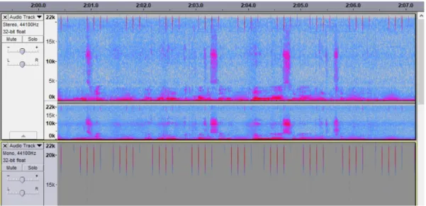
Figure 5- Audacity screenshot featuring spectrograms of the reference signal (bottom) and the recordings from mic1 and mic2 (top). The ultrasonic clicks are visible in every channel.

Setup for Collecting OptiTrack data

Physical setup: OptiTrack is a system of cameras and markers used to track detailed motion. To track a specific object in space, the user needs only to create a unique marker configuration, affix the marker to the object they desire to track, and register the object within the OptiTrack system. We created two markers, one to track the motion of a subject’s hand, and another to track the position of their head.

(17)

17

Figure 6 - Images of a user wearing the OptiTrack head and hand markers; The headset (blurred) is on the couch but is worn during the trial.

Software setup: OptiTrack provides its users with a python script to extract raw data from a constantly running data-stream produced by the OptiTrack system. For this project, we edited the python script to ensure each data packet had a corresponding timestamp. Standardizing the format of the packets enabled the data to be compatible with the scripts I wrote to analyze the motion data.

4.3. Tools Built and Used

Tools for Data Collection

In order to collect data at a high level of detail, we used a very high sample rate and avoided preprocessing the data unnecessarily. While preprocessing may have allowed us to see real-time plots of our results, it would have resulted in multiple lost packets, hindering us from capturing all the details of the data. To gather high fidelity data with minimal preprocessing, we opted to use off-the-shelf solutions to gather the audio and motion data, instead of building tools from scratch.

(18)

18

To record audio, we used Audacity, a well-established, fairly-stable, open source audio recording and editing program. Using Audacity enables us to collect clean audio data at a sample rate high enough to pick up the ultrasonic frequencies. The hardware used to record audio

records 16 channels of audio data. One channel is the reference channel which is simply the original signal sent out by the system. The reference channel is useful when observing the deformation of the click after its echoed back to the microphones of the headset. The other two channels, mic1 and mic2, are the information from the two microphones on the headset. These audio streams represent the ultrasonic echo information. It is beneficial to compare mic1 to mic2 because these microphones are located on different portions of the device. This difference in location of the microphones means that one can expect to see a difference in the reflected signals received by each microphone. This difference in reflected signals can later be used to discern more information about the position of the hand.

To record motion capture data, we used the data collection script and NatNet client provided by OptiTrack. The default data collection script provides information on the positions and orientations of all the defined markers within view of the sufficient number of OptiTrack cameras (the markers do not need to be within line of sight of every single camera in the space). We added a single line of code to the default script in order to timestamp every frame of motion data. OptiTrack’s python script outputs the data as a .txt file. We made sure to give the .txt file a name which corresponds with the audio file for the trial, and to put them in the same folder.

In order to collect ultrasonic echoes, we needed to generate the original ultrasonic click signal. To generate the ultrasonic clicks, I created a python class called Clicker. Clicker wraps and expands upon the foundational code built during the work previously done to develop the hardware-based groundwork of this project. The Clicker class generates an audio signal

(19)

19

consisting of a specified number of clicks per second at a specified frequency. The signal is then saved to a WAV file for use during both the rough and detailed data collection trials. The user can call the play() function on any clicker object in order to play the generated audio file. If a user calls play() and an audio file with the specified characteristics has already been created, the script will use the previously saved file to play the audio. If not, the script will generate the audio file, then play it. The user can also manually navigate to the saved audio file and play the audio file using their audio player of choice. For this project I often used Windows Media Player for this purpose.

Tools for Analysis

I built several Jupyter notebooks in order to visualize various characteristics of the recorded ultrasonic click echoes and motion data collected during various gestures.

Audio Analysis

To analyze audio, I built a Jupyter notebook in python called AudioAnalysisNtbk.ipynb. The notebook is outfitted with various functions for visualizing, parsing, and analyzing the data. The most important functions are detailed below.

AudioAnalysisNtbk performs the following steps on the audacity data to convert the audio into a usable form:

 Scans the folder for all audacity projects

 For each project it:

o Isolates the channels corresponding to mic1, mic2, and the reference audio o Deletes all unnecessary channels

o Amplifies the audio

(20)

20

o Saves a new copy of the audacity project for later use

After building a folder of FLAC files for each Audacity project (1 Audacity project = 1 round of data collection), the script, takes in a trial name and creates a “Trial” object which associates the name with the relevant audio files for the processed audio. Each Trial object is initialized with placeholders for arrays of Measurements which represent all the clicks in each of the audio files.

Trial

Trial is a class which holds and describes the raw information gathered from the audio portion of a detailed data collection trial. An instance of the Trial class holds the following information for its corresponding data collection trial; the trialname which is written in a standardized format, the path to the directory which holds all the necessary audio files for each audio channel, the cutoff frequency for the high pass filter applied to the audio files, numpy arrays for the filtered and unfiltered version of each audio file, and arrays of instances of Measurements for each audio file. To create a Trial instance, the user needs only to provide the trialname and path to the source directory.

Measurement

Measurement is a class which holds and describes the information for individual clicks within audio trials. Every audio trial can be broken down into three sets of Measurements, the set of all Measurements, the set of Measurements of just the big clicks, and the set of Measurements of just the small clicks. A Measurement contains the following information for a specific click from an audio trial; timestamps for the beginning and end of the measurement window, arrays of the audio samples within the measurement window for each channel, the norms of those arrays

(21)

21

calculated using numpy’s linalg.norm() function, arrays of the differences between subsequent samples within the window, and norms of those difference arrays. Measurements are created and applied to a trial when Process Trial is called.

Process_Trial

Process trial is the function responsible for parsing the information from a Trial instance. Process trial runs through the requisite audio files, breaks them down into windows, and creates a Measurement instance for each window. After creating all the Measurements for every audio file in a trial, process trial updates the Measurement arrays for the Trial instance. If a user processes a trial with filtered measurements, then later wants to work with unfiltered measurements, they must run process_trial again with do_filt set to false instead of true.

Process_trial works as follows. Based on a specified window_size and step_size, the script runs through the 'ref' flac file breaks it down into windows. The system finds the maximum value of each window, then it determines the timestamp of the point where that maximum value occurred. Then, for each mic signal (mic1 and mic2), the system goes to the timestamp and extracts a window of audio samples. This window should contain the information for a single click. The sample window is then used to create a Measurement with the characteristics described above. The following diagram depicts this process.

(22)

22

Figure 7- Workflow for sample window extraction

After running through the reference file there should be a list of Measurement objects (1 Measurement = 1 window = 1 click). The original signal contains two types of clicks; every big click is followed by a small click. Thus, the script creates two additional lists of measurements;

(23)

23

a_measurements, and b_measurements. Isolating clicks of the same size allows the user to run analysis on clicks of the same type. Centering the sample window around the max value from the reference signal enables the system to detect any temporal shifts due to the distance a click travels before being echoed back.

The idea is that if the hand is not moving successive frames should be approximately identical. Thus, the norm of the difference vectors should stay around 0 unless the hand is

moving. We can then graph this norm of differences over time to identify when (and hopefully to what degree) the hand moves. To illustrate this observation, I created some functions which build an animation of the sample frames from a trial.

Animate_sample

Animate_sample is a function which takes a processed trial and created animations based on the trials measurements. The process takes all the measurements in an audio sample and plots them one by one. Each plot is a single frame. Since every measurement, represents a click, the resulting image will appear to be mostly stable with intermittent perturbations. The amount of perturbation increases whenever the frames correspond to a moment where the subject was moving. This function enables users to visualize the deformation of the echoed click over time as a subject is performing some motion.

(24)

24 MultiAnimate

Multi_animate works like animate_sample but allows the user to overlay information from various trials over one another in the resulting animation. For example, one could animate the clicks from the reference channel and the mic1 channel. The resulting GIF will contain two waveforms differentiated by color.

Figure 9 - Example frames from click animation which overlays information from multiple audio sources

Plot_Audio_Data

Plot_Audio_Data allows the user to visualize the information from measurements across an entire audio file, or across sub-segments of the audio. With this function a user can create graphs of the norms of, Measurements along an audio file, the differences between

Measurements of an audio file, and the norms of differences along an audio file. Helper functions

Some other useful functions written for this portion of the project were:

 a high pass filter

 get_audio_trials, a method which processes entire folders of data

(25)

25

Motion Data Analysis

I built a Jupyter notebook called OptiAnlysisNtbk.ipynb responsible for parsing, analyzing, and visualizing the .txt files produced by the OptiTrack python script. The key functions from this Jupyter notebook are described below.

Measurement

Measurement is a class. An instance of a Measurement represents a single packet of information received from the OptiTrack script for a single timestamp. A Measurement records the time which it was received.

RelativePosition

Relative Position is a subclass of Measurement which represents the position information gathered from a single packet from the OptiTrack script. A RelativePosition Measurement holds the relative position of the user’s hand with respect to their head using a 3-element array

representing the relative x,y,z coordinates. RelativePosition also holds the orientation of the hand relative to the head using a 4-element quaternion.

RelativeVelocity

Relative Velocity is a subclass of a Measurement which represents the motion

information which results from the analysis of pairs of subsequent RelativePositions from the OptiTrack data. An instance of RelativeVelocity holds information on the relative velocity of the hand with respect to the hand as a 3-element array.

(26)

26 getOptiTrakData

GetOptiTrakData is the function which parses the information from the text file produced by the OptiTrack script. As it parses the text file, it builds a list of dictionaries where each

dictionary represents a single packet of information. getPositions

GetPositions takes a list of dictionaries representing OptiTrack packets and creates a list of RelativePosition objects.

getVelocities

GetVelocities takes a list of instances of RelativePositions and creates a list of RelativeVelocity objects.

plotOptiData

This function enables a user to visualize the motion data gathered from an OptiTrack trial. Given a list of Measurements and a string indicating what type of Measurements the user wants to plot; the function builds a color-coded plot including information on each parameter of the Measurement over time. The graph also includes a plot of the norm of all the parameters combined. For example, a graph of RelativePositions would have red, green, and blue lines representing the x,y,and z locations of the hand relative to the subject’s head with respect to time. The graph would also have a black line which graphs the norm of those three values over time. The norm of the x,y, and z coordinates of position yields the Euclidian relative distance between the hand and the head of the subject.

(27)

27

Lining Up Graphs from the Two Sources

The last Jupyter notebook I built for detailed data collection is called GraphAlData.ipynb. This notebook was built to enable users to visualize the audio and motion data simultaneously. The main functions within this notebook are get_all_data and plot_all_data. In order to use the code written in the aforementioned notebooks, I wrapped the code from the previous notebooks into classes within a couple standalone python scripts. I was able to import those classes into this notebook in order to parse the data from Audacity and OptiTrack.

Get_all_data

Get_all_data takes in the path to the source directory holding the Audacity and OptiTrack files for multiple trials. It goes through all files and parses them using the functions described above. Each trial’s data is named according to a standard naming convention which simplifies the process of joining together the audio and motion data for a specific trial.

Plot_all_data

Plot_all_data takes data from get_all_data, the trialname which specifies which trial to graph, and a list of the types of plots to include in the resulting graph. Plot_all_data’s purpose is to create combined graphs of the motion and audio data for a trial in order to enable the user to analyze correlations between the two. When collecting the Audacity and OptiTrack data, the user must rely on their ability to start both systems at the same time if they want the data from the two sources to line up temporally. Realistically, most people won’t consistently start the two systems at exactly the same time. To account for this, plot_all_data has an argument, time_shift, which allows the user to offset the audio data from the motion data in time. This allows a user to manually inspect and line up the graphs from the two sources, making up for any initial offset introduced to the data by starting the systems at different times.

(28)

28

Time Aligning Data Automatically

A method of automatic data alignment we began to explore was the use of a sort of robotic flashbang. The plan was to build a robot consisting of a motor and a speaker. Upon the press of a button the motor would move and the speaker would emit a beep. A unique OptiTrack marker could be placed on the motor and the beep can be set to a specific frequency that would not get lost in noise. Then, at the beginning of a detailed data collection trial, the user could start Audacity and the OptiTrack script, without needing to make sure they started at the same time. After starting the two systems, right before the user performs any actions, they press the button which activates the flashbang robot. The motor moves and the beep plays. The motion will show up as a specific set of packets in the OptiTrack data and will line up with the beep on the

Audacity file. The beep can be singled out in the audio stream through the use of a band-pass filter centered around the desired frequency. These corresponding markers in the motion and audio data can later be used to align the two data streams automatically.

4.4. Detailed Data Collection Trial Methods

After building all of the tools necessary, an example of an overall workflow used to collect detailed motion and audio data can run as follows.:

 Start the OptiTrack data collection script

 Start an Audacity recording

 Start the ultrasonic click audio

 Perform and repeat actions as desired

 Stop the recording and the clicks

 Save the recording with the convention: "Trial###--YYYY-MMM-DD-SubjectName.aup"

(29)

29

 Save the .txt file outputted by OptiTrack with the same convention.

 Place the Audacity files and the OptiTrack output into one folder

 To analyze the data, run the functions described in the tools section

4.5. Results

Motion Data

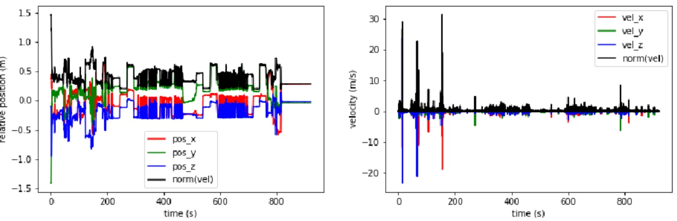
After finalizing the workflow, we set ourselves up in Bose’s OptiTrack room and collected some data. I ran the TXT file generated by the OptiTrack system through the motion analysis notebooks. The following graphs depict the processed data from those trials. The red, green, and blue, lines of each graph represent the x, y, and z components of their respective vectors. The black line represents the norm of the x, y, and z values.

Trial000

(30)

30

Figure 11 - Data from Trial000, zoomed-in to a single sequence of actions.

Trial001

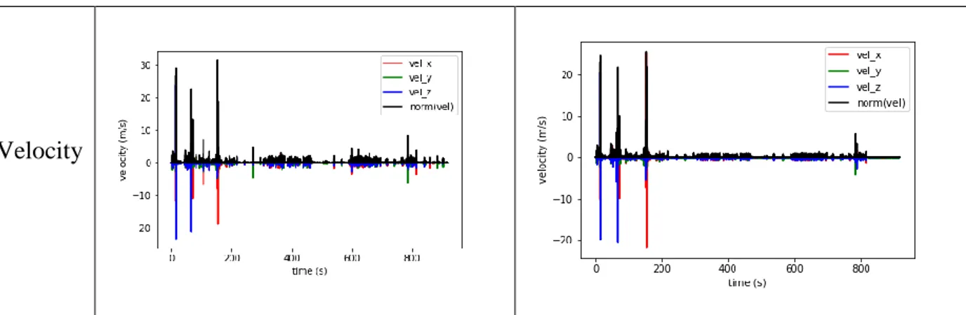
Figure 12 - Motion data from Trial001, position (left) and velocity (right), graphed over the course of the entire trial

(31)

31

Timestamp Adjustment

The moments when the subject has their hand close to, and far away from their ear are clearly visible on the position graphs. The velocity graphs are fairly noisy, but do provide some information as to whether or not the hand was moving at that moment in time. The noise may be due to some error in the timestamps generated by the OptiTrack script. Upon inspection, these timestamps do not increment in a regular fashion. In some cases, subsequent samples even had the same timestamp.

In order to attempt to reduce the noise present in the velocity graphs, we plotted the information using manually calculated timestamps instead of those automatically generated by time.time(). When manually calculating the timestamps we assumed the first sample began at 0 seconds and incremented by 1/120 seconds for each subsequent measurement in accordance with OptiTrack’s sample rate. We found no difference in the position graphs, and a slight reduction in noise on the velocity graphs.

Automatic Manual

(32)

32 Velocity

Figure 14 - Comparison of Trial000’s motion graphs generated using different types of timestamps, automatic (left) and manual (right).

OptiTrack Manual

Position

Velocity

Figure 15 - Comparison of the motion graphs generated using different types of timestamps, zoomed in to a small sequence of actions

(33)

33

Audio Data

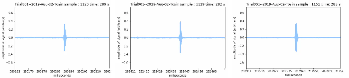
To illustrate the deformation of the echoed audio signal, the audio analysis script generates animations which visualize how the reflected signal is altered over time. Pictured below are a few frames from one of those animations.

Figure 16 - Key frames of the 'b' clicks from mic 1 during Trial001

These frames are all from one of the two types of clicks (big and small), specifically these are ‘b’ clicks. If the animation included both ‘a’ and ‘b’ clicks the animation would appear to flicker. The animation of clicks from the reference signal does not appear to change over time because the click output is consistent. In contrast to the reference clicks, the echoed clicks received by the mics constantly change and shift. Our hypothesis is that the transformations on the signal received by the microphones are caused by the motion of the hand.

An Interesting Observation

When looking through the animations generated from Trial001's data we observed an interesting phenomenon. The number of lobes in the reflected audio signal appears to depend somewhat on the volume of the original signal. This phenomenon can be observed when comparing two frames of successive clicks, one big and one small. The reflection from the big click has 6 lobes, while the reflection from the small click only has 5. This difference serves as a

(34)

34

possible explanation as to why our reflected signals look different during the rough data collection trials because we use a much lower volume for that portion of the project.

Big Click Reflection Small Click Reflection

Figure 17 - The number of lobes in the reflected signal depends on the volume of the source audio.

The difference in the number of lobes suggests that the frequency composition of an echoed click may vary with the intensity of the source audio. The following screenshot depicts spectrograms, produced by Audacity, of a big click and a small click from two data collection trials. The window on the left is from a detailed data collection trial where we played the audio a fairly high volume. The window on the right is from a rough data collection trial where we played the clicks at a fairly low volume. These images suggest that, as the volume increases, lower frequencies (10-20 kHz) feature more prominently in the echoed click. The click at the highest volume, the big click from the detailed data collection trial, features those lower frequencies at the highest level of intensity.

(35)

35

Figure 18 - Screenshot of spectrograms of individual clicks. The window on left depicts clicks played at high volume, the one on the right features clicks played at a low volume

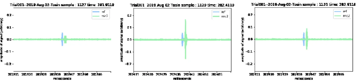
Comparing Signals

In order to compare clicks from the reference audio to the echoes picked up by the mics, I wrote a function which builds animations that consist of information from multiple signals. The frames featured below depict ‘b’ clicks from both the reference audio and mic2 during Trial001. As expected, while the clicks from mic2 change over time in response to motion, the reference signal remains constant.

(36)

36

Graphing the Audio Data

As mentioned in the tools section, one should be able to graph the norms of audio the vectors in order to identify when, and how much, the hand moves. The audio analysis script calculates two norms for each Measurement, the norm of the audio sample window, and the norm of the difference between sample windows. Because the windows should generally be identical overtime, the difference should be near 0 unless the hand is in motion. Thus, one can identify the moments when the hand moves by graphing the norms of the differences between frames over time. The following graphs are of processed audio data from Trial001.

Norm of the Audio Sample Vector

Norm of the Difference between Vectors

Whole Audio

Zoomed Portion

Figure 20 - Comparison of processed audio norm and norm-difference graphs

(37)

37

Analyzing the OptiTrack Data with the Audio Data

One of the ultimate goals of this project is to correlate audio signals with the motion of the hand. An initial step towards that goal is to manually inspect the data to identify any obvious correlations between the audio signals and the motion data.

In Trial001, there are several instances where the motion of the hand corresponds to spikes in the audio graphs. This correlation is made more apparent when comparing the velocity graph to the audio graph. The following images illustrate this observation. Spikes in the audio graph correlate to both, spikes in velocity, and the motion of the hand as it transitions between positions. We are unsure of what caused the blips in the audio graph which are visible in mic1's data but are not as prominent in the data from mic2. Potential causes can range anywhere from defects in the hardware to a bug in the audio plotting scripts. Locations on the graphs where there is motion data without accompanying audio data are indicative of times when we were setting up or using the OptiTrack gear without any ultrasonic audio playing.

(38)

38

Figure 21 - Comparisons between processed audio data and OptiTrack motion data (position – Top, velocity – Bottom)

The labeled points in the graphs above correspond to the following positions:

 Point A - hand moved from lap to ear

 Point B - hand moved from ear to far from head w/ outstretched arm

 Point C - hand moved from far from head to a period of constant cycling motion

The Issue of Time Alignment

When conducting the experiment, the OptiTrack data collection script and Audacity were not started at exactly the same time. If we started the OptiTrack script before Audacity, time t = 0 in the audio graphs would actually relate to some t > 0 in the OptiTrack graph. For the graphs above, we needed to manually account for the discrepancy in time alignment in order to identify correlated points. The following chart shows the times where the correlated points occurred in each of the graphs. During the data collection sessions, we used a phone alarm to signal when to switch between hand positions. Thus, to get the times for transition points in the Audacity file we just needed to search for places where the alarm went off. The consistency in the difference between correlated points strengthens our belief that they are related to each other, and not erroneously identified. (All times are in seconds.)

(39)

39

Point Raw Audacity OptiTrack Graph Audio Graph

A 237 247 240

B 257 270 260

C 280 292 282

Table 1 - Timestamps from various sources for points A, B, and C of the aforementioned graphs

This chart features data from Trial001. For every graph there is about 20 seconds between points A & B, and about 22 seconds between points B&C. The consistent 2-3 second delay between the audacity and the audio graphs may be due to the amount of time it took for the subject to mentally process the signal to switch hand positions. The difference in timestamps between the OptiTrack and audio graphs implies that the OptiTrack script may have been started about 10 seconds before Audacity was set to record.

Because Trial000 was our first attempt at data collection, we spent a lot more time setting up. As a result, Trial000 contains a much larger time alignment discrepancy than that of Trial 001, and is harder to find correlated points for.

Ideally, future iterations of this experiment should have a system which aligns the two sets of data automatically. In the absence of an auto-time alignment system, I built a python notebook which graphs OptiTrack and audio data together. The user can then manually shift the audio graph in order to manually time align it with the OptiTrack data. The following graphs feature combined position and velocity data from Trial000. The motion data in each graph is overlaid with audio data.

(40)

40

OptiTrack + Audio OptiTrack + Audio w/ -30s shift

Figure 22 - Subset of position and audio data from Trial000, all values are scaled to be between 0 and 1

OptiTrack + Audio OptiTrack + Audio w/ -30s shift

Figure 23 - Subset of velocity and audio data from Trial000, all values are scaled to be between 0 and 1

As previously stated, it was difficult to find a time-shift between the motion and audio data for Trial000. However, the graphs above do suggest that, at periods where the hand is most stable, the mic receives the least audio; and at times where the hand is moving quite a bit, the mic data exhibits multiple audio spikes.

A more promising correlation can be seen in the combined data graph below which features data collected from Trial001. Because Trial001 was our second attempt at data

(41)

41

collection, the process went more smoothly and resulted in a smaller time discrepancy between the OptiTrack and Audacity data. The following graph only needs an offset of 10 seconds to line up the audio and motion data.

Figure 24 – Zoomed-in portion of graph which features overlaid position and audio data

This graph depicts a clear correlation between the audio and position data when the user moves their hand rapidly back and forth. For every spike in the position graph, there is a

corresponding spike in the audio graphs for both mic1 and mic2.

4.6. Preliminary Conclusions

The detailed data collection sessions provided a decent amount of useful information. The system’s ability to successfully pick up the ultrasonic echoes confirms the preliminary findings from the COMSOL models.

Analysis of individual frames of the click animations showed that there are

distinguishable differences between the echoed clicks which depend on the position of the hand in relation to the headset. Observing the animated sequences of clicks showed how a change in

(42)

42

position of the hand is reflected by large changes in the form of the reflected click signal.

Building upon this finding, graphing the change in click shape over time illustrates the moments where the hand was in motion. To graph the change in click shape over time, we calculated the difference between every pair of subsequent frames. Then we graphed the norms of these

differences over the course of the audio sample. Thus, we could visualize the motion of the hand via the information gained from the audio signal. Large motions, signifying transitions from one hand position to another, are depicted as spikes in this norm-difference graph. Small motions, like those shown by pulsing the hand repeatedly by the ear, show up as series of small spikes in the audio norm-difference graph. These findings will serve to guide our analysis of the data collected from the rough data collection trials.

5. Rough Data Collection

5.1. Overview

After establishing a correlation between motion and audio, I sought to lay the

groundwork for building functional gesture classification models with the information we had gained. In order to use the correlation between motion and audio for practical gesture

recognition, we needed to collect a lot more data. The goal of the rough data collection portion of this project is to gather that large body of data in an environment that more closely mimics how an ultrasonic gesture recognition system would perform in the real world.

5.2. Design

The vision for the coarse data collection process was to create a system which walks users through various specified gestures and automatically handles much of the preprocessing in the background. To maximize the potential amount of data we could collect, the process was

(43)

43

streamlined such that, after an initial demonstration from the conductors of the study, subjects could come back and donate data whenever they had free time. Once the program is up and running on the machine, the users need only to input their unique ID and run through the data collection process. Every trial is also assigned a unique ID; trial IDs are used to differentiate between individual trials submitted by the same user. User IDs are used to anonymously group trials by user, and to differentiate between users. Grouping trials by user was done in case one wanted to use the data set to explore whether ultrasonic echo data, which gets transformed differently by the ear from person to person, can be used with machine learning for

identification.

In addition to building the data collection workflow, generating a large body of data is a major goal of the rough data collection portion of the project. The hope is that a significant amount of coarsely-labeled audio data can later be used to build machine learning models capable of classifying position and motion. The detailed data collection process using the OptiTrack system provided high fidelity data, but required a lot of time, was not very portable, involved coordinating schedules, and did not allow subjects to submit data on their own. In comparison, the rough data collection system takes only a couple of minutes to run through, can be set up anywhere, and users can submit data on their own whenever they would like. Thus, the rough data collection system is significantly more conducive to collecting the large amounts of data required for future work in this space, i.e. building machine learning models for gesture recognition.

In order to further maximize the amount and variety of the data we gathered, we had the subjects run through the motions twice with two sets of audio tracks. One audio track consists only of the ultrasonic clicks; the other track is a combination of simple jazz-like music with the

(44)

44

ultrasonic clicks overlaid onto the track. The ultrasonic echoes are later extracted from this signal through the use of high-pass filter. Using two audio tracks doubled the amount of data we could gather from the subjects of the study. Including the track with background music enables future research into whether ultrasonic gesture recognition models can be made resistant to noise.

Figure 25 - Setup for rough data collection featuing, the GUI, position markers, and headset (blurred out)

The preceding image depicts the setup for the rough data collection process. To begin, the user sits in line with the “head” marker. Once situated, the user either inputs their ID or indicates that they have not yet been assigned an ID number. The RoughDataCollect python program then walks the user through all of the motions, plays the ultrasonic audio, handles the Audacity

recording via the AudacityPipe class, and records relevant timestamps.

To carry out the vision described above we used built tools that carried out the following functions:

(45)

45

o I used the pygame library to build a clear and simple GUI capable of walking users through the data collection process.

 System for gathering data

o The RoughDataCollect python script runs all the processes required for data collection.

 Instructions for users to remind them of any detailed instructions (i.e. where each hand location is with respect to their ear, etc.)

o RoughDataCollect displays the instructions to the user via the pygame powered GUI. I also provided participants with a printed out set of setup and troubleshooting instructions.

 System for parsing data

o RoughDataParser is the python script I built to clip and label the data generated by RoughData Collect.

 System for auto-labeling to ease the downstream process of making classification models

o RoughDataParser automatically labels the data it parses.

 Generalized animation for manual audio analysis

5.3. Tools Built

Tools for Data Collection

I built three python scripts which work together to carry out rough data collection. Two of the scripts are class definitions, AudacityPipe and Clicker. The third script is the main code for running rough data collection. The third script employs both the AudacityPipe and the

(46)

46

Clicker classes as it walks the user through the various actions and records timestamps for all relevant events.

Audacity Pipe acts as a wrapper around the publicly available Audacity Pipe code provided by Audacity. The Audacity Pipe establishes a connection between a python script and Audacity, enabling users to automate series of Audacity operations via python code.

Clicker works as described in the detailed data collection tools section.

The program which employs the aforementioned classes and manages the entire process of rough data collection is RoughDataCollect. Rough Data Collect operates using the following functions and classes.

DCManager

DCManager, or Data Collection Manager, is responsible for running the overall data collection process. In order to carry out continuous data collection one needs only to make sure that Audacity is open, declare an instance of DCManager, and call DCManager.run().

DCManager’s run function effectively acts as the main function for the application. DCManager generates the IDs for a user and the trial, starts up instances of DCSessions, and carries out the functions responsible for displaying text in the GUI.

DCSession

A DCSession, or Data Collection Session, handles a single rough data collection trial. Once DCSession.run_session() is called, the program starts a new Audacity file, ready to begin the data collection trial. For each audio track, the DCSession walks the user through each hand position, prompting them via text shown on the GUI. DCSession records the beginning and ending timestamps for each motion within a dictionary that is later exported to a JSON file. At

(47)

47

the end of the data collection session, DCSession stops the audio tracks, saves the timestamp JSON file, and filters, exports, and saves the audio files from Audacity.

Prompts

All text prompts displayed through the GUI employ the function,

DCManager.show_text(). Show_text takes in all the desired lines of text and displays them centered in the GUI window. An example of a prompt can be seen in the image below.

Figure 26 - Example of a position prompt from the rough data collection GUI

Some prompts require user input. These prompts don’t use the show_text function but follow the same format. The key difference is that they have an extra rectangular element within the bottom half of the window which represents the text box for user input. As the user types, the letters they input are displayed in the “text box”. If the user’s text wouldn’t fit inside of the original size of the text box, the box grows to accommodate the user’s input. This feature is less pertinent for the ID entry prompt, and more useful when we ask the user to input any feedback they may have about the session. On the feedback page we also ask the users to input whether or

(48)

48

not they were wearing earplugs, that way we can later sort through those who wore earplugs and those who didn’t in case earplugs have some bearing on the characteristics of the echoed signal.

Tools for Data Analysis

The following scripts and functions were used to carry out the parsing, visualization, and analysis of the data generated by RoughDataCollect.

RoughDataParser

RoughDataParser.py contains the definition of the Clipper class. Clipper takes as input the audio files and the timestamp JSON from a Rough Data Collection trial. Clipper then cuts up the audio into individual audio clips for each motion according to the timestamps in the JSON file. Every resulting audio clip is labeled with its corresponding motion, this set of labeled audio files can be used to build various machine learning models. However, the clips may require some preprocessing which can be handled by the following functions.

AudioAnimate

AudioAnimate.py is a generalized form of the animate_sample function defined in the detailed data collection code. AudioAnimate enables the creation of the same click animations and can work with any audio file.

FlacCreator

FlacCreator.py goes through all of the Audacity files from a folder of Rough Data Collection trials and breaks them down into individual FLAC files for each channel of audio, (reference, mic1, and mic2).

(49)

49

FormInput

FormInput.py is made up of functions for use in the ModelBuilder. This script’s main function is to format the frames from the processed audio clips which a user intends on using as input for various machine learning models. Form_input has functions which can take a stream of frames from an RDC Trial and output an array which represents some transformed version of those frames, e.g. the norms of those frames, the differences between those frames, norms of the differences between those frames, spectrograms of the frames (useful for analysis of the Doppler characteristics of the altered audio signal based on the motion of the hand), and more. Every function in the script follows a standard format. Thus, this script is designed to be expandable so that users can define more possible transformations for their input arrays.

FrameFinder

FrameFinder.py runs through all of the audio clips from a rough data collection trial, breaks the audio clips down into frames, and saves the frames as numpy and TXT files (in a CSV format). The idea behind this script is to enable easy visualization of entire audio clips, as oppose to the frame by frame animations produced by AudioAnimate. Saving frames as numpy arrays saves time later when the frames need to be accessed during model building. The frames mirror the Measurements from the detailed data collection trials.

ModelBuilder

ModelBuilder.py is used to generate graphs of the processed data from RDC trials as well as to build machine learning models. The machine learning portion of this script is meant to act as a framework for the sequence of steps required to take output from an RDC trial and use it as input into a machine learning model. At the tail end of this project I managed to build a couple

(50)

50

example models to test out the framework. Future researchers who hope to use this data set to build more robust models can take this framework and adjust it to best fit their workflow.

ModelBuilder.py contains the definition of the SampleScraper class. An instance of SampleScraper has a function which enables it to run through and parse folders generated by RoughDataCollect.py. To retrieve all of the samples, for a specified label, from a folder of rough data collection trials, the user needs only to run SampleScraper.get_samples with the requisite arguments.

In order to work with the large sets of data involved in ModelBuilder more efficiently I created a python notebook, ModelBuilder.ipynb, which features all of the same functions that are included in ModelBuilder.py.

5.4. Rough Data Workflow

Figure 27 - Rough data collection workflow

To begin a rough data collection trial, whoever is managing the data collection must make sure Audacity and the Rough Data Collect script are running. Once all the software is

(51)

51

setup and running, the user is instructed to sit in line with the head marker. The user then puts on the headset and, optionally, an earplug. To begin that particular data collection session, the user either inputs their unique ID number or indicates that they do not yet have one.

Figure 28 - User inputting their ID at the beginning of a data collection session, the headset is on but obscured by the user's hair

The system reminds the user of their ID, then sets up a new Audacity recording in the background. At this stage the program enters a loop which is carried out for each position – close, mid, far, and lap. On each iteration of the loop, the system tells the user where to place their hand, and plays beeps to indicate the beginning and end of the position. All of the actions are done twice, once with just the ultrasonic clicks playing, then again with the combined ultrasonic clicks and music audio. At the end of the session, the program asks the user for feedback, stops the Audacity recording, and saves a JSON file which holds all of the timestamps for the positions during that trial.

(52)

52

5.5. Results

We ran about 40 viable rough data collection trials. In total, we actually ran a little over 40 trials but some of the sessions needed to be scrapped due to various errors such as; dropping the headset, stopping in the middle of the trial, etc. Each trial consists of two sets of audio, just clicks and clicks with music in the background. Each set of audio had users place their hand in 7 positions: close, mid, far, on their lap, far again, mid again, and close again. Running the

positions in this sequence enabled us to gathered extra information on every position, as well as some information on the transformations of the signals during the transitions in each direction, inward and outward. Every position is held for about 5 seconds, and we played clicks at a rate of 50 per second (25 big and 25 small). Thus, if we call every click a frame, we succeeded in collecting approximately 40*2*7*5*50 = 140,000 frames of labeled data.

From the detailed data collection trials, we learned that the methods of analysis which provided the most information were observation of the shape of the echoed clicks, and graphing the norms of the differences between frames over time. Therefore, while I included functionality to process the data in a variety of methods, for this paper, I will focus on the results pertaining to the shapes of the clicks and the norms of the differences between clicks across audio samples.

In order to observe the shape of the echoed click, I used the frame_average()

transformation from my form_input python script. Frame_average takes all of the frames from an audio signal (represented as an array of arrays), and outputs the average along the entire click. The following images depict examples of the “average click” collected over the audio clips from various hand positions of the rough data collection session for a single subject.

(53)

53

Close Mid Far

Figure 30 - Average echoed click at each position for a single user

The lobes present in the reflected echoes from the detailed collection trials are also present here. However, the noise makes them hard to see. To make the signals clearer I took the average of the “average clicks” across a subset of all of the rough data collection trials. The graphs below show the averages of the “average clicks” across 10 of the over 40 rough data collection trials which we ran.

Close Mid Far

Figure 31 - Average echoed click at each position across multiple users

These waveforms are much cleaner, making it easier to see the individual lobes. The number of the lobes is not exactly the same as the number seen during the detailed data collection trials. However, during the detailed data collection trials, we found evidence which suggests that the number of lobes seen in the echo is closely tied to the volume at which the original signal was played. For the rough data collection trials, the volume of the clicks was about 10-13% that of the detailed data collection trials. Thus, the presence of fewer lobes makes

(54)

54

sense. Because we held the volume constant across all of the rough data collection sessions, we can fairly accurately compare the results across the sessions.

Close Mid Far

Figure 32 - Average echoed clicks at each position across multiple users, zoomed into click

The preceding graphs demonstrate that the main portions of each echoed click consist of two lobes. However, as the hand gets further away, the size of the first lobe decreases. The graph for the average “mid” position click has an extra set of smaller lobes offset from the main pair. These extra lobes could be from another echo from the hand implying the signal managed to travel from the speaker, to the hand, off the subject’s head, back to the hand, and back to the microphone. The graph for the average “far” position click also has a secondary set of lobes which are smaller and farther away from the main pair (visible in Figure 31). This lines up with the secondary click seen at the mid position, since the hand is held farther away, it would make sense for the secondary click to be farther and smaller. Continuing with this logic, there is

probably also a secondary echo present in the signal from the “close” position, but since the hand is so close to the headset at this position, the secondary echo comes at approximately the same time as the primary one, and thus gets overlaid on the graph.

Spectral analysis of the average click waveforms provides some insight into a possible explanation for the difference between the average click waveforms at each position. The graphs below are the spectrograms produced by taking the Fourier transforms of the average clicks