Circulations and water mass balances in the Brazil Basin

(1)

CIRCULATIONS AND WATER MASS BALANCES IN

THE BRAZIL BASIN

by

Huai-Min Zhang

M.S. Institute of Atmospheric Physics, Academia Sinica (1987)

Submitted in partial fulfillment of the requirements for the degree of

Master of Science at the

MASSACHUSETTS INSTITUTE OF TECHNOLOGY and the

WOODS HOLE OCEANOGRAPHIC INSTITUTION September 1991

@

Huai-Min Zhang 1991

The author hereby grants to MIT and to WHOI permission to reproduce and to distribute copies of this thesis document in whole or in part.

Signature of Author.. .... . ... .. ... ...

Joint Program in 1 ysical Oceanography Massachusetts Institute of Technology Woods Hole Oceanographic Institution August 26, 1991

Certified by ...

...

r...

Nelson G. Hogg Senior Scientist Thesis Supervisor Accepted by ... ... Lawrence J. Pratt Chairman, Joint Committee for Physical Oceanography Massachusetts Institute of Technology Woods Hole Oceanographic Institution

(2)

CIRCULATIONS AND WATER MASS BALANCES IN THE BRAZIL BASIN

by

Huai-Min Zhang

Submitted in partial fulfillment of the requirements for the degree of Master of Science at the Massachusetts Institute of Technology

and the Woods Hole Oceanographic Institution August 26, 1991

Abstract

Based on the Levitus atlas, we find that the application of the Montgomery streamfunc-tion to the isopycnal surfaces induces an error which can not be ignored in some regions in the ocean. The error arises from the sloping effect of the specific volume anomaly along isopycnal surfaces. By including the major part of this effect, new streamfunc-tions, namely the pressure anomaly and main pressure streamfuncstreamfunc-tions, are suggested for the use in potential density coordinates.

By using the newly proposed streamfunction and by including the variations of specific volume anomaly along isopycnal surfaces, the inverse model proposed by Hogg (1987) is modified for increasing accuracy and applied to the Brazil Basin to study the circulation, diffusion and water mass balances. The equations in the model, i.e. the dynamic equation, continuity equation, integrated vorticity equation, and conservation equations for heat, salt and oxygen (in which a consumption sink term is allowed), are written in centered finite difference form with lateral steps of 2 degree latitude and longitude and 8 levels in the vertical. This system of equations with constraints of positive diffusivities and oxygen consumption rates is solved by the inverse method. The results indicate that the circulation in the upper oceans is consistent with previous works, but that in the deep ocean is quite different. In the NADW region, we find a coincidence of the flows with the tongues of water properties. The diffusivities and diapycnal velocities seem stronger in the region near the equator than in the south, with reasonable values. Diffusion plays an important role in the water mass balance. Examples show that similar property fields may resulte from different processes.

Thesis Supervisor:

Dr. Nelson Hogg , Senior Scientist Woods Hole Oceanographic Institution

(3)

Chapter 1 INTRODUCTION

1.1 Overview

The investigation of the ocean circulation is very important in the study of the heat transport in the ocean and thus the global climate system. Unfortunately, direct mea-surement of ocean currents, especially those in the deep oceans, is extremely difficult. On the other hand, hydrographic data, such as temperature, salinity, oxygen, etc., are much more accessible. Thus one primary task for oceanographers is to deduce the ocean circulation from the available hydrographic data.

Understanding the physical mechanisms for balances in the water properties is not only itself an important topic, it is also essential for the inference of the circulation from the hydrographic data (water properties). For example, if one believed that advection is the only process in the water property balance, one would infer that the flows are along the isopleths of the property. On the other hand, if processes other than advection, like mixing due to diffusion etc. are also present in the balances, as is almost always true in the ocean, one must utilize a different approach to infer the circulation.

Traditionally, there are two approaches to deducing the ocean circulation from hydrographic data: one is the descriptive method (water mass analysis or the "core

(6)

method"), and the other is the dynamic method. In the descriptive method, the fields of the water properties (such as temperature, salinity, oxygen, etc.) are used to deduce the circulation configurations. In Wiist's (1935) core layer method, the extremes of the water properties are interpreted as the primary "spreading" pathways of the flows. The isentropic analysis (Montgomery, 1938) is another example of the descriptive method. Since the distributions of water properties generally depend on both advective and diffu-sive processes, the water mass deduced flows can only give us a flow pattern in a general sense, but cannot correctly give us the detailed structure of the flow field. On the other hand, in the dynamic method, the distributions of the density field are used to derive the shear flows or relative flows through the hydrostatic and geostrophic equations. To get the absolute velocities, the so called "reference-level" or "level-of-no -motion" issue must be resolved. Early attempts to obtain the reference level velocities are based on the assumption that there must exist some levels at which velocity vanishes, such as the ocean bottom, an interface between two water masses which appear to flow in opposite directions, and so on. But there are no dynamic justifications for the existence of the level of no motion. An alternate attempt to get the reference level velocities is to measure them directly, but again there are practical difficulties.

By using the conservation equations for mass, heat, salt, carbon-14 and oxygen in a box model, Wright (1969) determined the deep water transports in the Western At-lantic. More recently, Wunsch (1977) applied the general inverse theories to the field of the oceanography to determine the reference level velocities; and independently, Stommel and Schott(1977) proposed the fl-spirial method to solve essentially the same problem, and this method was further developed by Olbers et al (1985). Instead of exactly sat-isfying geostrophy (implied by solving the reference velocity), as in the two previous works, Hogg(1987) combined the dynamic method with the conservation laws for the water properties to determine the absolute velocities(actually the streamfunctions) at all levels simultaneously by the least square fit or the inverse method. (More detailed

(7)

comparisions among these models are discussed in the following sections). Calculating the velocities relative to the ocean bottom initially, and then adding and adjusting the so called barotropic components to the relative velocities to make the flows consonant with the property distributions and mass conservations, Reid (1989) determined the adjusted steric heights for the absolute flows and transports in the South Atlantic. His model and results will be discussed in Chapter 4 for comparison with our model results.

1.2 Comparisons of the Inverse Models

The basic assumptions in Wunsch's box inverse model (1977, 1978) are that the oceans are in hydrostatic equilibrium, flows are in geostrophic balance, and the conservative water properties, such as mass, heat, salt, etc., are conserved in closed volumes. The mathmatical expressions for the first two assumptions are

- -gp (1.1) 9z fv = (1.2) p ax fu = -- . (1.3) p Oy

Combining these equations yields the "thermal wind" relations:

f V -g-p (1.4)

az

p

ax

foa

g i8p

f -U _ - - (1.5)

i9z p Oy

Integrating the above equations with respect to z from the reference level, zo to any level

z , we get the absolute velocity at the level z as

9 tzap

fV(X, y, z) = fV(x, y, zo) - Z -dz (1.6)

p JzO Ox

fu(x,y,z) = fu(x,y,zo) + J dz (1.7)

(8)

Substituting the above expressions for u and v into the conservation equations for the water properties, we obtain a simultaneous equation system concerning the unknown reference velocities, and the solutions can be obtained by the inverse method he used. Unlike the models discussed below, Wunsch (1978) generally applies the conservation laws over large closed volumes so that the data noise may be smaller (mass conservation is more accurate in large volumes than in small volumes). These box models are especially

good at determining velocities and transports across the hydrographic sections, but not

particularly suitable for determining the interior (within the boxes) flows.

In the f-spirial method postulated by Stommel and Schott(1977), in addition to the basic assumptions in Wunsch's model (hydrostatics, geostrophy), it is also explicitly

assumed that sea water is incompressible: 1

au

oo om

-+ + 0. (1.8)

8x~ Dy Dz

and that the density equation is in the conservation form (for the steady state and without diffusion):

Op

u-+o-+w-=0 (1.9)

Dx Dy Dz

Reorganizing all the above equations, and expressing the density gradients by the slopes

of the constant density surfaces(h = h(x, y)), the

#-spirial

equation is derived as

02h D2h

p

u ±o( -- )=0 (1.10)

8xoz Oyaz

f

'Note that if the compressibility of the sea water is considered, nondivergency Eq.(1.9) is still a good first order approximation, but the density equation may have more complicated form than Eq.(1.8). Ref.

(9)

Principally, the absolute velocities at all depths can be obtained in the following way. Firstly, the direction of the velocity at all depths is given from Eq.(1.10) by

V 82h a 2h 3

tanO

- - - -

/(

)

(1.11)

Secondly, if one of the coefficients of u and v in Eq.(1.10) vanishes without the other vanishing at a particular depth, then obviously that component of u and v which is associated with the non-zero coefficients also vanishes at that depth, and thus the level of no motion for that component is decided. Therefore the absolute velocities for that component at all depths are consequently determined by the thermal wind relation, and the other component is likewisely determined by the direction relation, eq.(1.11).

In practice, the coefficients for u and v are not well determined because of the large data noise which has impacts on the second order derivatives. Actually, in the application of the f-spirial method, instead of finding the level of no motion, an equation system for the velocities (uo, vo) at a previously selected "reference level" is formulatted as follows. Decomposing the absolute velocity V at any depth into the known shear velocity V, , which is obtained from the density field by the thermal wind relation, and the unknown reference velocity

VO,

substitution into eq.(1.10) yields

82h i92h 9 2h _ 12.h

o + VO( ) = - (1.12)

8 xo9z

oyoz

f

roxoz VByoz

f

This equation can be applied at any grid points where the derivatives 4.2, hy, exist, so that a system of equations for uo, vo is derived, and the solutions can be obtained by the general inverse method (But this is generally overdetermined because there are just two

(10)

unknowns). As in Wunsch's model, conservation equations for other water properties can also be added to give more constraints to the solution. The work by Olbers et al (1985) is one example. Different from the box model, the conservation equations are written on a point-wise basis.

In all the above models, the unknowns are the velocities at the reference levels. The absolute velocities at all other levels are then calculated using the thermal wind relation. This implies that geostrophy is satisfied exactly in these models. In the oceans, geostrophy is a quite good first order approximation for the large-scale flows (Pedlosky,

1987), thus the real ocean flows may deviate from geostrophy to some extent. Based on essentially the same assumptions as above, but instead of calculating the reference velocities, Hogg(1987) formulated a model to determine the absolute velocities(actually the streamfunctions) at all levels directly. By computing the velocities at all depths simultaneously, the artificially enforced exact satisfaction of geostrophy is relaxed. The extent to which geostrophy is satisfied depends on the relative weights for the dynamic equations and other conservation equations(this can be seen from the data resolutions). In the present work, Hogg's model is first modified to make it more exact for the potential density coordinates, then the model is applied to the Brazil Basin to study the circulation and diffusion processes in that region. A more detailed discussion of the assumptions and formulations of this model is given in Chapter 3.

1.3 The Brazil Basin

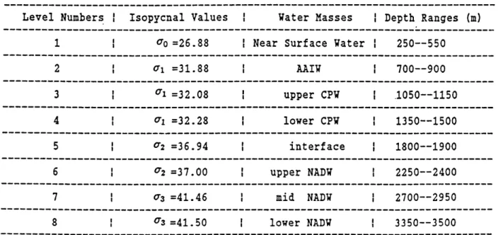
The Brazil Basin is chosen as the region to apply the model, because in this basin there are many uncertainties about the circulation and mass conversion processes. The Brazil Basin contains a rich water mass structure, namely: the central water in the surface; the Antarctic intermediate water(AAIW), circumpolar water(CPW), Antarctic bottom water(AABW) from the south; and the North Atlantic deep water(NADW) from the

(11)

north. Even more water masses can be idenfied by the extremes of the water properties. All these waters meet in the Brazil Basin, flowing over and mixing with each other in the interfaces to adjust their characteristics. Nevertheless, the exact pathways of the flows and the mechanisms by which the water masses are modified are still unclear. Because of the large and complicated vertical distributions of the water properties, mixing may be the important process in the water property conversions, which not only has direct significance on the tracer distributions, but also has significance on the circulation through its impact on the stratification of the ocean(Tziperman, 1987). However, there are many physical processes which can be responsible for the mixing: from mesoscale eddies to small scale turbulence, and to molecular diffusion. In the case where only molecular diffusion is important in the mixing, double diffusion may als6 be effective because of the different diffusivities for heat and salt (Turner, 1973). Schmitt (1979) shows that the salt fingering is mostly active when 1 < R, < 2, where R, = aO6/3S,

is the ratio of the density fluxes due to heat and salt. The profiles of Rg() shown in Fig.1.1 suggest that at some depths double diffusion is potentially important. Because other processes, such as wave breaking, cabbeling, etc. (Turner, 1980), may also occur, the actual effectiveness of the double diffusion depends on the relative strengths of all

these processes, and is still an open question.

The purposes of this work are try to answer some of the questions raised above. In Chapter 2, a new, appoximate streamfunction for the potential density surfaces (hereafter defined as isopycnal surfaces) is deduced based on the data analysis. Chapter 3 gives a

detailed description of the model, and a brief discussion of the Levitus atlas and basic

techniques in the inverse model used in this work. The model results and their analysis are presented in Chapter 4, followed by a brief summary and remarks.

(12)

RP = 13

-10.0 -8.0 -i.0 - .0 -2.0

-*

es-2.o 4.0 6.0 a.0 10.0

(13)

Chapter 2 STREAMFUNCTIONS FOR POTENTIAL DENSITY

SURFACES

2.1 Introduction

A well known fact about the oceans is that the flows and mixing are much stronger in the horizontal than in the vertical. Thus it is possible to find surfaces along which the veloc-ities and mixing have their major components while those across are minimized.The very early choice of such surfaces is the potential density surfaces (Montgomery, 1938), where the potential density is defined as the density a fluid parcel would have if it were isentrop-ically and adiabatisentrop-ically moved to an arbitrarily chosen but fixed pressure, for example, the ocean surface pressure. Although the in situ density p generally increases monotot-ically with depth, which means that the ocean is statmonotot-ically stable, inversion of potential density gradient is still possible, because the static stability is not simply determined

(14)

by the gradient of potential density (Wist,1933;Ekman,1934). 1 Ekman(1934) proposes the use of potential densities at different depths with reference to different pressures, and

even suggests notations a1, o₂,etc. which are widely used till today. By definition, fluid

parcels having the same potential density can be freely moved around on the reference pressure surface p, without experiencing buoyancy forces. However, with respect to the in situ pressure, there is no such property. Recently,McDougall (1977) suggested the use of the neutral surfaces, which are defined as the surfaces on which small isentropic and adiabatic displacements of a fluid parcel do not produce buoyant restoring forces on the parcel. In principal,these are the surfaces we want. But in practice,the computation and interpretation of the neutral surfaces are far more difficult than that of the historically used isopycnal ones. As neutral and isopycnal surfaces coincide at the reference pressure, if the potential densities at different depths are with reference to different pressures, and if the in situ pressure is never allowed to be more than 500 dbars from the reference pressure, the deviation of the isopycnal surface from the neutral surface should be small. Therefore,the more commonly used isopycnal surfaces will be used in this work.

Streamfunctions for several different vertical coordinates have been found, such as pressure for geopotential surfaces, dynamic height for pressure surfaces,Montgomary streamfunctions for steric (specific volume) anomaly surfaces and for steric or in situ

density surfaces (McDougall, 1989). Nevertheless, exact streamfunctions for isopycnal surfaces have not been found yet. In his work,Hogg(1987) applied Montgomary stream-function on isopycnal surfaces. The data analysis presented in the later sections shows

'The criterior for static stability in terms of potential density is such that

-N2 =-C -_ B-- > 0 (2.1)

9 pe dz dz

where N is the Brunt-Vdssals frequency,C = aP( ),,s, B = -(jg),p,, and S is salinity.See Gill(1982) for detail.

(15)

that this application implies that a potentially important term has been neglected. By in-cluding the major part of this term in the Montgomery streamfunction, an approximate, but more accurate streamfunction for the potential density coordinate can be obtained which will be derived next.

2.2 Operators in Potential Density Coordinates

To work in potential density coordinates,it is necessary first to derive the expressions for the linear oprators in this system. In an arbitrary curvilinear (orthogonal) coordinate as shown in Fig.2.1,the general three dimensional gradient operator is

VA - (- A

H1

8l1 1 8A 'H2 862' 1 OA )3 19 (2.2) S const. I

Fig.2.1 A Curvilinear Coordinate the three dimensional divergence operator is

-. 1 a(H2H3A1) 8(H3H1A2) 8(H1H2A3)

7H-A = { + + +) ],A

(16)

and the three dimensional Laplacian operator is

19X

H C__ )2 S=const. -1 * H2 A = ₃ H1 H2H3 j=1 H1H2H3aA 8( l --- )8(

a.

[(1)2 + ( )2 C8( + (± )2Oy + (± )2]-1. 8:

.jL..

Fig.2.2 Relation Between Coordinates (z, y, z) And (1, 2, 0)

For the o--coordinate (hereafter,o- represents the potential density surfaces, which

can be o6 or o-1 to 0-4), as shown in Fig.2.2, the o- surfaces are generally so gentle that we

can make the following approximations:

(1 =x-cos9 - z.sin? X.1 - z.- X + z

0%~ X , (2.6)

and similarly,

- y,

S = (x,y, z)- , and thus Z = z(x, y, o)

where (2.4) (2.5) (2.7) (2.8) (2.9) + (X ~)2

(17)

Using the above approximations, we have H 2 ₁₂ ₊ _{02 +} ₍ ₂ 22 Hi= 02 + 1 Oz 2 H = (-) Oz 2 + _(---) = ;H3 =

-Be,

1+ (,X)2 oyz 1+ ( )y2 , 2 S1 ;H1 1 S1 ; H2 ~1

Therefore, the 3-D gradient and divergence operators in the u-coordinate are

OA -8A V A = i- ₊ 3j--S-A = ax2 + Oy -8A koz- - = V,A + O OA3 + ]- - pV-^ A kaz OA3 + O

where V, and Vh are the 2-D lateral gradient and divergence operators defined in the a-coordinate: .0 - O I _{^x + j} y Vh uez ₁ Ox T + j

By Oz

]

Partial Differential Relations between the z-coordinate and the u-coordinate

In the two different coordinates, any property A can be expressed as

A = A(x, y, z) = A(x, y, z(x, y, o)) or A = A(x, y, a) = A(x, y, (x, y, z)) (2.17)

Hence the partial differential relation can be derived as

OA OX 8A By (2.10) (2.11) (2.12) (2.13) (2.14) (2.15) (2.16) 8A Oz

+

az Ox), OA Oz Oz Oiy (2.18) (2.19) =

(18)

or, in terms of the 2-D gradient operator,

8A

VZ A = VA - V-- ,z (2.20)

B9z

2.3 Streamfunctions for Isopycnal Surfaces

In this section, we will first figure out the error term associated with the application of the Montgomery streamfunction to the isopycnal surfaces. Then using the Levitus atlas values, we will show that this error may not be negligible in some regions in the ocean. New streamfunctions will then be proposed for the isopycnal surfaces. Note that in this work,the streamfunction is not conventional (which implies horizontal, or more precisely, two dimensional nondivergent flow); instead, this streamfunction is defined for

f

V which

implies fV is nondivergent,and in the -plane, divergence of the lateral flows may be allowed.

We start our derivation with the general geostrophic relation in the z- coordinate, i.e.

-1

-k x fV = -- VZP (2.21)

p

where k is the unit vector in z direction,V is the 2-D lateral velocity,and Vz is the 2-D gradient operator in the z-coordinate. In an arbitrary vertical s-coordinate (e.g., s = -),

by applying eq.(2.20) and the hydrostatic equation(!2 = -gp),the above equation can be written as

1 8p

k x

fV

= -- [VP - -

7,

z]

(19)

1

= -['VP +

gVz]

P

-[a V,

p

+

v,(g

-

z)] (2.22)

where a = . is the specific volume. Generally, a reference level is needed when using the

p

geostrophic relation. Assume Vr is the geostrophic velocity at the reference s,.-surface, i.e.,

k x fV, = -[a V, p + V,(g -z)],, (2.23)

then we have

k x f(V -Vr) = -[a V,p - a V, p, + V,(g - (Z -Zr))J

S-[aV. p - a, V. pr - V, a - dp] (2.24)

in which the hydrostatic equation has been used. Using the specific volume anomaly defined by

6 = a(S, T, p) - a(35, 0, p) = a - a, (2.25)

where S and T are salinity and temperature respectively,and a, = a(35,0,p) is the

specific volume for the standard seawater at S = 35 psu and T = 0*, thus a, is a function of p only, then the above equation becomes

-I

xf( -r) = -[6 9,P-6, VsPr + aV~p- a, - 6-dp- 6-p P a, .dp]

(2.26)

Note that

9, a, -dp= P,v) a,(p') dp' = aP p p -- a,,p , (2.27)

(20)

then eq.(2.26) becomes

kxf(V-Vr) = -[sVp-rV p, - V, 6 - dp] , (2.28)

i.e. eq.(2.24) is also exactly valid for the specific volume anomaly 6.

In short-hand notation,and keeping in mind that eq.(2.28) is a relative relation between two s surfaces, we can simply write it as

(P-kxfV

=

-[6

V

p -

V, J6

-dp]

,

(2.29)

= -[a

vp-v, f

a - dp].

(2.30)

As examples several known streamfunctions can be derived from eq.(2.29) or

eq.(2.30) directly:

A. For s = z being the geopotential surface,the second term in eq.(2.30) vanishes by the hydrostatic equation.Thus

k x pfV = - 72p (2.31)

and the streamfunction for pfV is simply the pressure p.

B. For s = p,namely the pressure coordinate, Vp = 0, and it is obvious that

(21)

and the streamfunctions for

fV

are the dynamic height or geopotential:

O,

= -

J

- dp , or O,= - -. (2.33)

p

C. For s = 6,i.e. the steric anomaly surfaces, the & can be taken into the gradient

operator, thus the Montgomery streamfunction is derived as

m = p6 -

6.

dp (2.34)

D. Also for s=a = _{j, we similarly get the Montgomery streamfunction for the}

in situ density coordinate:

b=P

P. (2.35)

P -P

E. However,for the isopycnal surfaces(s = o-) since 6 is generally a function of

(x, y) on these surfaces, thus a closed or precise form for the streamfunctions cannot be

derived. How large will the error be if we apply the Montgomery streamfunction on the isopycnal surfaces?Taking 6 into the gradient operator, eq.(2.29) can be manipulated to become

(22)

The first two terms are just the two components in the Montgomery streamfunction, thus the last one will be the error term:

ERM

=

pV0, 6,

(2.37)

Table 2.1 shows the ratios of this error term to the gradient term of the Montgomery streamfunction between two isopycnal surfaces oi = 31.8 and ui = 32.3 in the

Mediter-ranean Water tongue region by using the data set of the Levitus climatological hydro-graphic atlas (Levitus,1982). It can be seen that in some areas,the magnitude of the error term can be as large as, and even larger than that of the Montgomery streamfunction gradient term, and more seriously even in opposite sign. One interesting fact that should be pointed out is that, each component of the two gradient terms of the Montgomery streamfunction

(V,(6p),

or -V, fP S-dp) can have a magnitude an order larger than that of the error term,but as the two components often have opposite sign , their residual is greatly reduced and generally of the same magnitude as the error term. Mathematically, although

()<

«1

(2.38)

v,.(Sp) V, fPS- dp ' we still have

v'7(~

O(1) (2.39) vo,(Sp - f P -dp

(23)

Table 2.1 Examples of ratio [p V, 6/

V,

(p6 - fp

o.

dp)]I in the Mediterranean tongue region (45.5 0W - 19.50W, 23.5*N - 45.50N). DW325-Fv=41_y 635~ 555 oT'~5W'-*M_4-- a 20-2.683--, 3 5-0069-0.1:---0101 0.0000 -0.2630 -0.2449 -0.4656 -0.5696 -0.8274 -1.1636 -1.4.598 -1.4353 -4.3047 -2.0099 -0.4450 -0.1416 -0.1274 -0.19(2 0.0000 -0.2000 -0.0)?I -3.3743 -0.5925 -1.2125 -1.5423 -1.7652 -1.5059 -2.8020 -1.6267 -0.407! -0.0740 -0.02(4 -0.0665 0.0000 -0.1727 -0.0069 -0.3141 -0.5836 -1.5125 -2.2764 -2.2366 -2.1332 -6.3966 -1.4639 -0.3033 0.0541 0.0675 0.0214 0.0000 -0.2262 0.0511 -0.1$!1 -0.5t43 -1.6332 -2.6510 -3.4218 -6.5580-12.3368 -1.5223 -0.0812 0.3345 0.1299 0.0271 0.0000 -0.2!17 -0.0380 -0.2348 -0.8046 -1.5.95 -2.5069 -6.5219-56.3030 -9.S582 -0.(094 0.2004 0.63t5 0.1394 0.0565 0.0000 -0.2C61 -0.3375 -0.53'! -1.0606 -1.6074 -3.6565 -5.2121 14.9683 13.9567 1.05(0 1.2906 0.8920 0.2704 -0.1577 0~-1373- 1 -21731- 1.8129~~ 1-5S475~- 1 .197 ~-- 1t45~~~2 -UrG3& _~=C 1903~-0-309 ~~A~I05-~ 1~-373 -= 2r.0 --0.0000 -0.9233 -0.7762 -1.3524 -1.3170 -2.1902 -3.3420-12.5314207.4020 -0.9112 7.8756 6.5554 1.63!6 0.7007 -0.472?7

-= -DO V_(~=1 -.&2 7 5~- 3. I9 71 SS- 5 5~131 3 5~-T 17709 85-_ C3728~~-0 .It 25~=0770 33~~=0 . 6 31--=1 .02 7 I~=1~ 330&6~

0.0000 -1.5395 -1.1437 -3.2!02 -2.6765 -4.3035 -3.9398 -4.8574 -3.6066 -7.6824163.6494-19.5544 AAa k 1.5992 -0.8372 -1.5535~=17B193 2.711~ C1839~=1-3989=C5130~~ C013=03 12=UTr.ES-=0~9258-=1.:049v1=1978

0.0000 -1.6749 -1.6435 -3.3393 -3.658-2-2.531 -2 .3908-27.3981-11.8009 -3.1331 -4.3700 2.9480 -1.0C66

-1.E53T 77759~-2:r335~=21 2~T35~13(~T~9~=7i~~053' _E9=739 33

0.0000 -0.8547 -1.4783 -1.9913 -4.1910 -6.7538 -4.1586 -2.9854 -2.7099 7.8673 -1.2415 -2.4406 -4.0486 1.6316 -0.9756 0.0000 -0.4534 -0.7620 -1.1004 -1.3052 -1.6366 -1.8810 -2.1461 -3.4625 4.7223 0.0945 -0.4627 -1.1811 -0.1868 -0.6573 0.0000 -0.4406 -0.4794 -0.5718 -0.7605 -0.9145 -1.0987 -1.6387 -2.9332 1.1488 0.43(6 0.1468 0.2047 -1.1060 -0.8428 0.0000 -0.3757 -0.4254 -0.4663 -0.5e11 -0.7003 -0.t253 -1.2594 -6.0455 0.9922 0.2666 0.1529 0.C016-23.535L -1.2450 c -T0aC~r~02a7--;0957~21.099 CI2~1T 9- ~325~1555= 36-G70T~=?0971~=C11 13 0.0000 -0.3)15 -0.!?24 -0.4724 -0.5450 -0.6023 -0.6795 -1.0719-10.4352 0.2479 0.0015 0.1537 0.4505 0.9173 -2.3520 ~3 37~ 23 1- 9033~1T~53T~79= 793- 1535~--I11U9~=70941 0.0000 -0.2837 -0.3550 -0.4340 -0.55!5 -0.6141 -0.6768 -0.8673 22.8660 0.0056 0.0003 0.0763 0.1.569 0.6555 25.3518

~ 1 -; C-? -5 3.~00 2 ~5 3-0 t(01~- 1-7 2 7 1~~ 3-5 37 7~5 T~95 50~~-0~D00 00~~57.B7 5 i~~0~.5 2 3 &~ - 2 2 9 T~=1I -10 9 1- V1-10 l.

0.0000 -1.053 3 -1.0129 -0.8522 -0.7!?2 -0.6768 -0.0039 -0.923! -6.9507 0.0874 -0.036S -0.0092 0.0710 0.4538 1.1010

~C9 % ~=~~7:35~7 0 C -. 0 03~2~37 ~ I3M -1. 21T83 . =115T~C -1fs~13-.-12170 71

0.0000 -0.1231 -0.0532 0.0299 0.1933 -3.2961 -1.3970 -1.1412 -1.6793 0.1401 -0.012 -0.000f -0.0222 0.1951 0.4765

~~2~~377Y~91 1~~T~~8E D~~=T~2T34 (T~23T3~ F0I3T 1985~rT~~~53T~1~T53V3~U1 7 8~1~~371 -l.2/V? 7

0.0G00 -0.0540 -0.0142 -0.0071 -0.0256 0.0142 1.0715 2.3243 -2.9795 0.2483 0.1095 -0.0680 -0.0091 0.0752 0.2473 0.E2EE~~~109~~=79T17C7E~~=7255;~1777~ T 33C~G3C~T78~-152~'1-5C155VY-0.060C -0.1ta6 -0.0515 0.0153 -0.05!9 -3.0156 -0.1(32 -0.!187 -0.6800 0.0007 0.01(2 0.1931 -0.0022 0.1380 0.1957 -U~C33~~~~T~~1763 o ~T7T20~-=T373 2~ T7 7 2 -3.1433~17~3I5"T~1i7V 1 .C53~-1-7718 3 0.0000 -0.0727 -0.1533 -C.01( -0.027' -0.0341 -0.1647 -0.5016 -0.!75 2.31E7 0.4371 0.366t 0.22(1 3.3051 0.2583 ~- E 107. 5 - ?70E-=2 1300

-0.0300 0.1411 -0.65o5 -3.20.6 -0.0912 -0.1031 -).O973 -0.13&9 -0.2356 -2.0512-11.7471 3.6256 U.4t!2 0.3752 0.2500

-- -36 i~-~0. 556 7~-9~-3 ',5-1-!3 ?4~ -~ 5 -~ .. ~6;12~--- 37 7 -3T4 3 35 ~-6~. !z a '---T '~v 9

75.5--0.Cc00 0.1240 -0. 0.17 -0.05S7 -0.2!49 -3.1ICC -0.1520 -0.156 -0.0935 -2.3208 -3.C123 1.I16? 0.8516 0.3694 0.X256

~UU~~~U.T2 .65~~~~075T6~ U73-.----TU55U ~~ .T3w Uf76 U151 ~~17V083~1 5201~-.7580

0.0000 0.1146 0.;0!! -0.157; -0.096! -3. ei 5 -0.2545 -3.2477 -0.2522 0.7584-15.0117 5.4345 0.6532 0.L!53 0.32'?

(24)

Table 2.2 Examples of ratio [p'v

61 v,

(p6 -

f

8- dp)]~ ~;;' in the Mediterranean tongue region (45.5*W - 19.5*W, 23.5*N - 45.5*N). F.7F7-0. -7653-6.21'13 0.0728 0.0452 0.0407 0.0483 0.0379 0.0366 0.0326 0.000 -0.0112 -0.007? -0.0300 -0.0.33 -0.1802 0.6234 0.2603 0.3670-.0.1550 0.3362 -0.0317 0.0246 0.0354 0.0411 0.0000 -0.0204 -0.011? -0.0297 -0.0S!S ' 0.346 0.1748 0.1696 0.2593 0.1460 0.2506 -0.0275 0.0133 0.0215 0.0241 GTD D ~~TD~5~~ ~Di2~~r23 1~-0~0 W -~-235 6.027F8 0.0377~~~5A278~~9 23-002~557 0.0030 -0.0336 -0.0202 -0.0354 -0.0571 0.1131 0.0894 0.1146 0.1456 0.0979 0.3099 -0.0241 0.0084 0.0100 0.0(090 .02 1 -0.0183 -0.0009 0.0000 -0.0463 -0.0273 -0.0346 -0.0761 0.1062 0.0706 0.0752 0.0735 0.0746 0.2499 -0.0097 0.0094 -0.0025 -0.0071 -0.7 -. 229 -0~T-T.T~~553 0.03- 0.0236 0.00235 03 F 01T2 2 0.0T0 0.6512 0.0000 -0.0613 -0.0420 -0.0527 -0.1t35 0.1147 0.0690 0.0516 0.0481 0.0577 -0.0966 -0.0015 0.0038 -0.0140 -0.0191 UK~53~-~3:T1n6 . 0.127T~~~6~T 2iT~~7 11S 0.FT51 0.0412 0. 0 T T -. b.-~ 17 C2C610 .-0.0000 -0.0908 -0.0904 -0.1C50 17.7384 0.1126 0.0465 0.0462 0.0322 0.0359 0.0112 0.0031 -0.0C74 -0.0219 -0.0294 -2 ~ ~~ 2 ~ ~ 31 T 5 TD58 0 .~~ 0.0000 -0.5362 -0.2L63 0.4391 0.1!30 0.0509 0.0337 0.0300 0.0277 -0.5(06 .0.0072 -0.0052 -0.0135 -0.0290 -0.0450 T0.13] 5 0.2 7 - 1 7~~~ -.11 ~ 2 ~~ 149~~5.152I 0.6000 0.2573 1.t748 0.0601 -0.0146 0.0134 0.0180 0.029? 0.0301 -0.0079 -0.0044 -0.0143 -0.0296 -0.0347 -0.0707 ~-0036~-0u3~1-000~~7077-0T--12--T2 1. -- 21 8~=~2027~3356~~~~ 35-1~~.255 0.0000 0.1294 0.1301 0.0215 0.0062 -0.0072. 0.0016 0.0230 0.0371 -0.0285 -0.0289 -0.0334 -0.0435 -0.0492 -0.0663 ~~.2059 -1.5T76 - ~ 0.0000--0.2559 0.0926 0.0233 -0.01.4 -0.0144 -0.0029 0.0152 0.0256 0.03e6 -0.1779 -0.0577 -0.0566 -0.0475 -0.3507 :1:n7T~~~~~077~0~0 190T~~U 110 0 326 TUU0 -0.7740 -D.1sF23 94 0~ 051~212 ~~TTT5 0.0000 -0.0757 -0.0545 0.1311 -0.0167 -0.0159 0.0007 0.0153 0.0176 0.0096 0.0249 0.0637 -0.3544 -0.0496 -0.0766 ~07 177 ~~0 0 5~~ ~ -27~0~.0 371 ~~~0 GS ~~ -D 45~~ M. T6 1.T~7 0T~~0~.;5 7. .0 ~3 69~~~ T i-3 1~~~ ~1335 0.0000 -0.0423 -0.03C6 -0.0236 -0.0064 -0.0196 0.0457 0.0141 0.0099 0.0027 0.0011 0.0082 0.0199 0.4410 -0.0789

S9 7~~~700599 64~51 1. 003 O7. 6 3 29 ~D 25 2U5 0 3- -D O5-92~~0~~7 7 4 .~5 03--1 559-~~0 11232(~~~ .I k Z ~

0.0000 -0.0322 -0.0237 -0.01a9 -0.0113 -0.0130 -0.0246 0.0161 0.0012 -0.0042 0.0002 -0.0003 0.0011 0.0058 -0.0004

(IGT~EU0 .66002~~311001 .2700T~~ 15~0 D93~~071 1 3~~~20?2

0.0003 -0.0248 -0.0116 -0.0095 -0.0076 -0.0014 -0.0049 -0.0266 -0.0031 -0.00&6 -0.0025 -0.0033 -0.0044 -0.0068 -0.0165

=0:i173~=070237~~0.078 1~0 173~~0:10303~~D~U20r U~03TT~~.~~573D~02t8~~ 5055~~~12 53~~~D2088

0.:000 -0.0007 0.0079 0.0023 0.30.5 0.0061 0.0035 0.0539 -0.0101 -0.0010 -3.0044 -0.0059 -0.0076 -0.0123 -0.0151 0~~uT77 3.~3T0:03 117~~0~3 7 0.J T~7:3TTE 005I0- 02T -37~23~~0.050 5-0-~119 F1071128

0.0003 -1.2596 -0.9365 0.o724 0.1070 0.0424 0.0725 0.2147 -0.0101 0.0025 -0.0022 -0.0G57 -0.0096 -0.0153 -0.0166 .0 1 -~~UT 7UT 0 00 ~~~-G~ .~7i 7 ~77Y U~'i U.U ~~00 2U~'~00T.8 3~~~07D79 5~~ ~U U7

0.0000 -0.0066 -0.01!6 -0.0231 -0.0324 -0.04,3 -0.0962 -0.1413 -0.02?7 0.0135 0.0025 -0.0052 -0.0056 -0.0173 -0.0211

-u157~0~021..~-ou~lo UTr13U-U:327-~3; 1U3r~1Uus7~~DU23jGw274 .02~~~Uo39o .05/3

0.0000 0.63?7 -0.0003 -0.0376 -0.3096 -0.0114 -0.02?7 0.0263 0.1213 0.0322 0.0042 0.0016 -0.0093 -0.0103 -0.0245 U > -007323 -U.2<J -0.01rY U.00 3 U.J142 0.277 7.0141 701U3 .0226 0.03 13003i5

0.0000 0.045. 0.00;0 -3.0027 -0.00 -0.0352 0.0077 0.0s62 2.0029 0.1021 0.0224 -0.0131 -0.0085 -0.0235 -0.0269 U-.n1 0:6 -0 . CT1--G~072 Cu~~UT 7 Tr4 3. 07- T1 90-0 T~702 -0703 U.

0.3000 3.0767 3.0527 0.0C1 0.3J16 -0.0001 5.01!4 3.0534 0.2434 0.1153 -3.0010 -3.C2c2 -3.C214 -0.0760 -0.0310

u-G3G7~=0~DT27~~~0~3 21~0 TIi -= -01 -=--5 ~~0~'S O ~ S.31-~0.0093~~0.:312 2-~ .01 5- .G23C-~

0.0.CO 0.6254 0.05.45 0.375S 0.019! 0.0135 0.0104. 0.021 0.0753. -3.011 5 -0. 1066 -0.046 -0.0.21 -0.03Sq -0.02;l

U-U502V 5 U -U7~~U.=~3TT-UCU. -0TT6 07 U.00Tm 5~~~~U70 5T-~~ U.D 11~0135

0.0000 0.0334 0.1430 0.1015 0.1255 0.0525 0.0301 0.02?3 0.321? -0.194E -0.1930 -C.0E70 -0.3dE -0.0370 -0.0307

*"ti- -u -rc2-5T-CTUl u !m l2~~"~3iT35'~T -U713 -. UU1 -UGU)T6~~~UTU3-~7UUr1 .--- U-0 . u

0.0000 0.1152 -0.0217 0.3020 3.1242 0.1752 0.1125' 0.0520 0.0705 -0.0936 -0.1?60 -0.1465 -0.3070 -0.0460 -5.0292

(25)

-From the above analysis,we see that the Montgomery streamfunction may not be suitable for the isopycnal surfaces in some regions. Note that the error term arises from the variations of the specific volume anomaly along the isopycnals. Since the climato-logical data set is used, one may doubt whether the sloping signals are really significant because of the data noise(errors due to measurements,averaging,ect.). Unfortunately, the data I have for the time being cannot answer this question. Another question that may be asked is whether it is necessary to include this error term compared with the terms neglected in the geostrophy assumption. The geostrophic relation for the large scale mo-tions in the ocean has been strongly supported both by theory (e.g., Pedlosky , 1987) and by observations (e.g., Bryden, 1977), thus we do not expect that the neglected time varying and nonlinear terms are in the same order as the Coriolis and pressure gradient terms. In conclusion, because of the large size of this error term, we believe it should not be neglected, and a streamfunction for isopycnal surfaces is needed.

The following discussions are not only true for isopycnal surfaces, but also true for any gently sloping surfaces.Define the pressure anomaly as

p' =P-P (2.40)

where p is the lateral mean pressure on the s-surfacethen by definition,

,P = 0. (2.41)

Then eq.(2.29) is identical to

/xfY =

-[vP'-v.,

6 -dp) (2.42)

(26)

If we now define an approximate streamfunction(hereafter labeled with pressure anomaly streamfunction) as

Oa = p"6 - .Sdy, (2.44)

then the error in the use of tb. on the s-surface will be

ER. = p'V, 6 (2.45)

which is proportional to the "residual" or anomaly pressure p'. For gently sloping surfaces (such as isopycnal ones),and if the surfaces are not too near to the ocean surface, i.e. if p is large enough, we generally have

ER _, _(2.46)

ERM P

and we would expect that the use of this streamfunction on the s- surfaces produces much smaller errors. Actually,as shown in Table 2.2,the Levitus atlas values shows that

V P'~ O(10 2 ~ 10- ) (2.47)

v,(p'S

-- fP

-dy)

Consequently we can conclude that the streamfunction

9.a

defined by (2.44) is a fairly good one for the isopycnal surfaces, with the errors of at most 10% or less. The only difference between the anomaly or approximate streamfunction 1,b and the Montgomery

streamfunction ?k is the use of the pressure anomaly instead of the total pressure in the term p6. The reason for this modification can also be clearly seen from eq.(2.37) in

(27)

the following way. We see that there are two parameters in the error term:the slope of the specific volume anomaly and the total pressure p.The slope itself is really small,it is the large value of p that makes the product comparable to the gradient term of the Montgomery streamfunction term.In the derivation of eq.(2.36), the error term -p

V,

6 appears by taking 6 into the lateral gradient operator V,. Therefore the p in this term acts only as a coefficient of the term V,8, because the lateral variations of p are still kept in the gradient of the product term 7,(p6).Therefore if we decompose p into

P

+ p', and for p'

< p,

the error term p V, 6 can be approximated by p V, 6 (with the error p' , 6)

.Using this approximation,eq.(2.36) becomes

kx

f

=

-[,(S) -

V, J

6 - dp -pV, 6]

= -vo p'S - 6-dp) (2.48)

and this again leads to the definition of

4.

Although the streamfunction 7P, is approximate for the generalized s-coordinate, the generalized geostrophic relation(2.29) is exactly true for all kinds of s-coordinates. To interpret this relation physically, the following discussion reveals that this relation is no more than the application of the dynamic relation (in the p-coordinate) to the generalized s - coordinate. For simplicity,we only discuss one component of eq.(2.29):

P2

_6.dp

₊ ₎₁ _(2.49)

f(V - V2) = ) 6-d+61 ),p1 - 62 ).P2 (.9

As shown in Fig.2.3, the pressures on the two surfaces si and S2 at the two stations

A and B are PiA, PiB, P2A and P2B respectively, and M1, N1, M2, N2 are separately the

mid-points between stations A and B on the pressure surfaces P1BP1AP2B and P2A

The dynamic relation on the pressure surfaces read as:

a

P2B 1 P2B P2I

f(VM1 - VM2) = 6 -dp ~~ 6B dp] 6A dp (2.50)

(28)

f(17N1 - 1"N2) = P2A P1A A 6.dp ~ 1[ P2A 86-dp L PI S- dp P2A PI A

Fig.2.3 Geostrophic Relations Approximating the velocity VN1), and on the 32 surface by V2

yields f(1'1- V2) I ifjP2.E = [L (P 1 = L PB 1 ['P2B 1 [2( 1 Pl + ( fP P1 P2B SP2B L PIB S t N2

Between Two Stations On The s - Surfaces

at the mid-point on the si surface by V ~

}(VMi

+ ~ .(VX2 + VN2) , then adding eq.(2.50) to eq.(2.51)

.P2A P2A P2B

B-d_ 6A -dp+dp-

+

_6A-dpJ

P1A p1A PiB

P2B P2A P2 6dp--/ 6-dp)+ P2(6B+6A)-dp B

J

Pi A ~ 'PlA P2 B - (8A+ SB) -dp] PIB 2B P2A SB -dp - SA -dp) B "PIA [P 2 A PlA +JP 2B)(S+6)d] +] )B+6bA)'dp-- (fA+B.d+ P2BB P1B p1A 8Bdp- _fP2A _Adp)+ P2A (bB + 8A) P1A P2B

JP1A

(SA + SB) -dp] PIB P2A 6B -dp

-

6 -

dp)

28 5 A -dpj (2.51)

(29)

+ (2A (p2A - p2) - (21A + p1B)(A - P1E)|

which is exactly the difference form of eq.(2.49).These argumests clearly indicate the geometric implications of V, and V2 .

From the above geometric arguments as shown in Fig.2.3, one may also expect the following approximation:

(2.53)

and thus the following approximate streamfunction for the s-coordinate:

0 = 8- dp

Actually, this is also follows. As shown in

P2/n

a good approximation, and can also be derived mathematically as Fig.2.4, note the integrating approximation that

dp = S-dp - - -d + 6-dp ~ j-dp - Sip' + 6_2p', _(2.55) Pi P' J Z.-CO?2~t P2 (Xy) F2 = const.

Fig.2.4 Integrating Approimations on the Gently Sloping s surfaces

(2.54) (2.52)

(30)

Using eq.(2.36), the geostrophic relation can be developed to k x f(Vi - V2) =

-[VP

2 6

dp

+

81 , sP1 - 62 V aP2] f1 = -[v,(] 6 .dp - 61pl + 62P') + 61 v, (i + p') - 62 V, (f2+ P'2)] = -[, 6-dp - p' V, 61 + P' V 62] (2.56)

In this equation, the last two terms on the RHS are exactly the error terms neglected in the definition of #b, and for the same reason they can be ignored here, hence the

ex-pression for the streamfunction is attained(hereafter labelled as mean pressure

stream-function).

To show the effectiveness of the use of the pressure anomaly and mean pressure

streamfunfunctionsthe 9.'s and 's for the isopycnals and the O's for the specific

vol-ume anomaly surfaces in the Mediterranean Water tongue region are computed from the Levitus atlas values and displayed in Fig.2.5. Also shown in this figure are the exact streamfunctions for the the specific volume anomaly surfaces(Montgomery streamfunc-tion) and for the pressure surfaces(Dynamic Height) as well as the Montgomery stream-function on the isopycnal surfaces. (The two values for 6 and p in Fig.2.5 correspond to their mean values on the two isopycnal surfaces).It can be seen that all streamfunctions show similar lateral flow patterns between the two depths except the one from the Mont-gomery streamfunction on the isopycnal surfaces. It implies that the errors on the use of the Montgomery streanfunction on the isopycnal surfaces are effectively large in the

southern part of the region.It also shows the use of Oa and on the isopycnal surfaces

is extremely good. In this work we will use the # as the streamfunction for the a-coordinate, because in deriving b, another approximation-the integrating approximation (however small the error) was used.

(31)

.2...1..

)<

-..j.a.m--.J-v--aWa.m -5-..-3.sa5-.s-.-3.u .ea-J.g-.-.as~- . s-. . 3.J-...3-.S-U.g..-.U-J.a-3.U-.j.3-M .. Ss-J-..s .-Ja.3..-a

LD8ITC LOIMTC

(a) . between oi = 31.8 and al = 32.3 (b) between ai = 31.8 and oi = 32.3

(c) fu between al = 31.8 and cI = 32.3

i.

0

(f) 0;, between p = 759.6 and p = 1335.9

For Different Coordinates

31

V

(e) between 6 = 89.0 and 6 = 52.0 Fig.2.5 Various Streamfunctions

(32)

2.4 SUMMARY

In this chapter, we showed that when the dynamic method is applied to isopycnal surfaces, the variation of the specific volume anomaly along isopycnal surfaces has dynamical importance. By considering this variation, two streamfunctions have been formulated for any gently sloping surfaces, such as the isopycnal surface, neutral surface and so on. One is the pressure anomaly streamfunction which is analogous to the Montgomery streamfunction,but the the pressure anomaly is used instead of the pressure itself, i.e.

I=p'6s- f dp (2.57)

The other is the mean pressure streamfunction which is analogious to the dynamic height, but the mean pressure is used instead of the pressure itself.

A2

Sdp (2.58)

These streamfunctions are defined for laterally nondivergent quantity fV:

k x fV = V, (2.59)

The lateral divergence of

V

itself is allowed. The application of these two streamfunctions on the isopycnal surface generally induces errors in velocity less than 10%.

(33)

Chapter 3 DESCRIPTION OF THE MODEL

3.1 Introduction

The model used in this work is basically the one proposed by Hogg(1987), which has the following assumptions: flows are in hydrostatic equilibrium and geostrophic balance; mass is conservative at each grid point (Continuity Equation), and mass is conservative between isopycnal surfaces (Integrated Vorticity Equation); water properties like heat, salt, oxygen (a sink or consumption term is allowed for the oxygen equation) etc. are conservative. Instead of calculating the two components of the velocity, streamfunctions are calculated. (One practical advantage of this procedure is that the unknowns associ-ated with the velocity field are reduced by half). Some modifications of the model have been made. Specifically, in the dynamic equation the new streamfunction for the poten-tial density surfaces which includes the variations of the specific volume anomaly on the isopycnal surfaces has been used to replace the Montgomery streamfunction; consistently, by considering these sloping effects, a new form of the integrated vorticity equation has been reformulated; an exact potential density equation has been deduced by considering the variations of the thermal expansion and saline contraction coefficients with temper-ature and salinity as well as the possible differences in diffusivities for heat and salt; finally, as more levels are included in this work, the controlling equations are written in

(34)

three - dimensional difference forms by a staggered finite difference frame (which will

be discussed in the following sections) which permits us to remove the derivatives of the diffusive parameters as unknowns. In this chapter, we will first present the formulations and their implications for the equations, followed by brief discussions on the Levitus atlas and inverse techniques.

3.2 Formulation of the Equations

3.2.1 Dynamic Equation

As discussed in the previous sections, the assumptions of hydrostatic and geostrophic balances result in the thermal wind or shear flow relation. In the a-coordinate and in terms of the newly defined streamfunction, this relation can be expressed as

7kk(x,y) - 7kk+1(z,y) = 'pk 6 dp + pkSk - Pk+1k+1,

where K is the level number of the isopycnals in the model. "Dynamic Equation" in this work.

k= 12,.. ., K - 1 (3.1)

Eq.(3.1) will be called the

3.2.2 Mass Conservations at the grid points-Continuity or Potential

Vorticity Equations

The complete or precise form of the mass conservation for a fluid parcel is

1 dp +. =

(35)

The sea water is compressible

('f

#

0), but it is generally believed that the compressibility is small compared to the divergence term, i.e.

1 dp

p <dt _1.

(3.3)

Therefore to the first approximation, sea water may be considered as three dimensinally nondivergent(the nondivergency is only in the sense of eq.(3.3), it doesn't mean sea water is incompressible), and the continuity equation is thus written as

V -V = 0. (3.4)

or, using the operators for the o-coordinate,

Vh - + 0z-- = 0- (3.5)

where u' represents the 2-D lateral velocity and the superscript * appended to w em-phasizes explicitly that w* is the cross isopycnal velocity. As discussed by Hogg(1987), eq.(3.5) can also be interpreted as the statement of the conservation of the potential vorticity (f ft, ignoring the relative vorticity) as follows:

Multiply eq.(3.5) by foz, we have

fcz Vh -d = -fOz 2_w*, _(3.6)

Note that

(36)

and that

Vh -(f Oz ) = (fU) = 0 , (3-8)

we obtain

. .v,(fc.) = fe,2 *, (3.9)

which states that the variation of the potential vorticity fo along the streamfunction is caused by the cross-isopycnal stretching term. Thus the continuity equation combined with geostrophy may also be called the potential vorticity equation.

Note that the streamfunction is defined for

fiT,

not for U' itself. Hence it is

fd

that is laterally nondivergent, thus Vh -U' also involves the divergence of the planetary vorticity

f,

and this variation can be expressed explicitly as follows. From the definition

k x= - - V, k (3.10) f or U= fk XV (3.11) we have 11 - = h x V?)

=-

-(k X &)+(iv x V.)- () ffo 1 - '7f = h - (- xV ) ( _x ₂ =Vh -Ug - Vg (3.12)

(37)

where fo is a local constant and u'g is laterally nondivergent, defined as

1 f

ug = .- k x V,= -i. (3.13)

fo

Therefore the continuity equation can be rewitten as

"#

ow*

h z- = 0. (3.14)

fo

o

This is the exact equation used by Hogg(1987).

3.2.3 Integrated Vorticity Equation-Mass or Potential Vorticity Con-servation between Two Isopycnal Surfaces

Eq.(3.5) is the statement of mass conservation on each individual isopycnal

sur-face. Our purpose is to establish an expression for the mass conservation between two isopycnal surfaces, and this expression is important because it contains the inhomoge-neous terms to give the system unique non-zero solutions (the only other inhomogeinhomoge-neous terms come from the dynamic relation, eq.(3.1)). For the same reason we introduced the new streamfunction for the potential density coordinates, the variations of specific volume anomaly and pressure on the isopycnals will be included in the derivation of the integrated potential vorticity equation.

Thermal Wind Relation in o-coordinate

In order to get the desired expression, the thermal wind relation in the 0

-coordinate is needed. Note that

(38)

the geostrophic relation, eq.(2.29) can be rewritten as

k x fd = p V, 6 -

7o,

p -

d6.

Differentiating the above relation with respect to o-, we get

k x

f

= p,, 6 +P =pV,6+P 86 0

V-,

v,(-O496

o1

_o,

J

₆

6 f p - d6) i.e. k x

f--

Oe fu O-O, 06 = p,-, Op 06 = +-T Op 06 0,49X 86 Op 06 Op + Oe Ox (3.18) (3.19) (3.20) (3.21)

These are the exact(no approximation used) thermal wind relations in the u-coordinate. Integrated Vorticity Equation

Dividing the continuity equation, eq.(3.14), by u., yields

a u

_{T( )}

_Ouz O

Oz

Ox Ocr) Ow* -9W 0 (3.22) V o

+

()+

w* 5j-7 0 .- (3.23) (3.16) (3.17) + (TV) +

(39)

8 1 0(U [ i(zu)

[-(zu) +-(zv)]+

a[ (zv) - z ]

YOAT

Ocr

The following operations

- Eq.(3.20)] +

a

_[Yz-

₇

1

_-

_Eq.(3.21)]

O

BO 1

y

o

₌₇

{[p(

.,-y.)

z

ea

( .y pS.] y (p,. 5,.}

f

For p in Pascal, we have z ~ -10- 4p. Substituting the z in the RHS of eq.(3.27) by

-10- 4p, recombining the terms, we get

0 onu

a(z )

+

a(z

0~

0v-

)

10-4 a

=

f

{

80

pp.y - py-i.)] + p(p,1. - 6,p)

f~LkazP~~~~T (3.28)

Substituting eq.(3.28) into eq.(3.25), we obtain

O 10-4 9 10-4#

ow*

[r Oxu)+ (zv)]+ [pf p -p )]

f

p(pS-68,p.)+T- = 0. (3.29) Hence OU

on

T'+

_+W

ow* _(3.24) =0.

)]+ 5.= 0.

0

Ou

onr

+

FY(zT+ 9 (3.25) -[z -Ox result in (3.26)

O

Onu

O(z x )+ (3.27)

Circulations and water mass balances in the Brazil Basin