Aftershocks in engineering seismic risk analysis.

ABSTRACT

AFTERSHOCKS IN ENGINEERING SEISMIC RISK ANALYSIS

by

HANS ARNOLD MERZ

Submitted to the Department of Civil Engineering on May 11, 1973 in partial fulfillment of the requirements for the degree of Master of Science.

This study deals with the role of aftershocks in seismic risk analysis.. The purpose of risk analysis is to assess the probabi-lity that the maximum seismic intensity experienced at a struc-tural site in a lifetime of T years will exceed a units. It has been noted in several historical events that certain sites located at some distance from the mainshock epicenter have experienced more severe shaking during the temporally and spatially distributed

aftershock sequence than during the larger mainshock itself; the cause is apparently the closer proximity of a particular aftershock to the site. _{This study evaluates this "additional aftershock} risk". The analysis of both main- and aftershocks accounts for uncertainty in the times, locations and magnitudes of earthquakes as well as uncertainty in the attenuation "laws" (correlations). Mainshock occurrences are governed by a homogeneous Poisson process

in time whereas the temporal characteristics are represented as a non-homogeneous Poisson process triggered by a mainshock and with parameters depentIent on the mainshock magnitude. Aftershocks are assumed to occur at random spatially in a region whose location and extent depend upon the (random) mainshock location and size.

Analytical expressions for the risk are given for two cases -of -s-pa-t-i-a-l--ass-ump-t-i-ons: ma-i-nshock-s-an-d aftershocks occur on a

"line" fault; and mainshocks occur on a line, but aftershocks may occur in a surrounding areal region. Because the analytical ex-pressions are complicated and difficult to evaluate, a method is presented to determine an upper bound on the risk from both main-and aftershocks. _{Numerical results (upper bounds) are given for} the simplest, first case and compared with a method that accounts

-3-only for mainshocks and a method that treats all earthquakes as mainshocks. The preliminary conclusions are that the contribution

of aftershocks to the seismic risk are in general small for large examined seismic intensities at the site (say, 0.lg or more), especially when only mainshocks of moderate to small magnitudes (7.0 or smaller) are anticipated in the future. However, it might be significant in regions where mainshocks are usually followed by a large number of aftershocks. In any case, risk analysis of both main- and aftershocks is complicated and the simplie method, which

accounts only for mainshocks, yields risk estimates adequate (but underestimated) for engineering purposes.

Thesis Supervisor: C. Allin Cornell

Associate Professor of Civil Engineering Title:

ACKNOWLEDGEMENTS

This research was sponsored by the U.S. National Science Foundation under Grant No. GK-26296.

-5-TABLE OF CONTENTS Title Page Abstract Acknowledgement Table of Contents List of Figures List of Symbols Introduction

Assumptions and Parameters of the Seismic Risk Model

2.1 Temporal Characteristics of Main-and Aftershock Sequences

2.1.1 Parameters of the Mainshock Occurrence Model

2.1.2 Parameters of the Aftershock Occurrence Model: Modified Omori Law

2.2 Magnitude-Frequency Law 2.3 Magnitude-Energy Law

2.4 Spatial Distribution of Earthquakes 2.4.1 Spatial Distribution of Mainshocks 2.4.2 Spatial Distribution of Aftershocks 2.5 Attenuation Law Page 2 4 5 8 10 Chapter 1 Chapter 2 12 18 18 19 20 22 24 24 24 25 26

TABLE OF CONTENTS (Continued)

Chapter 3 Derivation of the Analytical Models 3.1 General Formulas

3.2 Seismic Risk Analysis of a "Line-Line" Occurrence Model 3.2.1 Special Assumptions

3.2.2 Derivation of the Analytical Expressions 3.2.2.1 Mainshock Analysis: Calculation of P[A] 3.2.2.2 Aftershock Analysis 3.2.2.2.1 Calculation of P[B] 3.2.2.2.2 Calculation of P[Al B] 3.2.2.3 Main- and Aftershock

Analysis of the "Line-Line" Model 3.2.2.3.1 ExactT Solution for py 3.2.2.3.2 Calculation of an U per Bound on _py

3.3 Seismic Risk Analysis of a "Line-Area" Occurrence Model 3.3.1 Special Assumptions

3.3.2 Derivation of the Analytical Expressions

3.3.2.1 Main- and Aftershock Analysis of the "Line-Area" Model Page 30 30 35 36 38 38 40 40 47 50 50 53 60 6U 62 62

-7-TABLE OF CONTENTS (Continued)

3.3.2.1.1 Exact Solution for pT y 3.3.2.1.2 Calculation of an U per Bound on p Chapter 4 Chapter 5 References Appendix A

Application of the "Line-Line" Model 4.1 Parameter Values of the Examples 4.2 Numerical Results

4.3 Discussion of the Results

Conclusions

Calculation of an "Average" Expected Number of Aftershocks per Year in a Particular Earthquake Source

Page 62 65 73 74 77 79 89 94 97

LIST OF FIGURES Page Figure 1-1 Figure 1-2 Figure 2-1 Figure 3-1 Figure 3-2 Figure 3-3 Figure 3-4 Figure 3-5 Figure 4-1 Figure 4-2 Figure 4-3 Figure 4-4

Spatial Distribution of Aftershocks in the Prince William, Ala-ska,; Earthquake of 1964 Spatial Distribution of Aftershocks in the San Fernando, California, Earthquake of February 9, 1971

Example of Main- and Aftershock Sequences in Time

Typical Fault-Site Configuration with a Typical Mainshock and its Aftershocks ("Line-Line" Model)

Point-by-Point Analyses of the Seismic Risk ("Line-Line" Model)

Typical Fault-Site Configuration with a Typical Mainshock and its Aftershocks

("Line-Area" Model)

Point-by-Point Analysis of the Seismic Risk ("Line-Area" Model)

Point-by-Point Analysis of E[naT] ("Line-Area" Model) y

Fault-Site Configuration of the Example Seismic Risk for the "Mainshock" Model Comparison of "Main- and Aftershock" Model with "Equivalent Event" and "Mainshock" Model for the case {m= 9.0, d = .30 km, va/%m = I.0}

Comparison of "Main- and Aftershock" Model with "Equivalent Event" and "Mainshock" Model: Variation of Upper Bound on the Mainshock Magnitude 16 17 29 37 37 61 61 67 83 84 85 86

LIST OF FIGURES (Continued) Figure 4-5

Figure 4-6

Comparison of "Main- and Aftershock" Model with "Equivalent Event" and "Mainshock" Model: Variation of Distance

Comparison of "Main- and Aftershock" Model with "Equivalent Event" and "Mainshock" Model: Variation of x = va/vm, where va = 'm = Constant

-9-Page 87

LIST OF SYMBOLS

p : Probability, that the maximum peak seismic intensity at the site exceeds y in T years y Seismic intensity (e.g., maximum peak

ground acceleration) T Time periods in years

{A} Event, that at least one mainshock in T years causes a maximum peak seismic intensity at the site in excess of y

{B} _{Event, that at least one aftershock in T years} causes a maximum peak seismic intensity at the site in excess of y

{C} Event, that at least one mainshock occurs in T years

T

E[nmT] _{Total expected number of mainshocks of interest} (i.e., causing a seismic intensity at the site in excess of y) in T years in an earthquake source E[nm : Total expected number of mainshocks of magnitudes

in excess of mm in T years 0

E[na T] Total expected number of aftershocks of interest y _{in T years in an earthquake source}

Probability that, given a mainshock occurs in a "point" source, the seismic intensity at the site will exceed y

pa _a Probability that, given an aftershock occurs in a "point" source, the seismic intensity at the site will exceed y

R _{Distance from a "point" source to the site} M, m : Magnitude

Mm, mm Mainshock magnitude

: Upper bound on mainshock magnitude m 1

-11-LIST OF SYMBOLS (Continued)

b

m m :Lower bound on mainshock magnitude ma Lower bound on aftershock magnitude

0

L Length of fault line

A91 Length of a (linear) "point" source Af Area of a (areal) "point" source Ay. : Length of intervals on fault line

E Energy of an earthquake

Parameter of the magnitude-energy law

W,

V : Average mean rate of occurrences of mainshocks (per year)

V Average mean rate of occurrences of aftershock a . (per year)

c, p, r Parameters of the modified Omori law t, t' : Time (in years)

'1' b2, b3 Parameters of the attenuation "law" E : "Error" term in the attenuation. "law" a : Standard deviation of ln c

D Linear dimension of potential aftershock area F Area of potential aftershock occurrences

6', y, 6 Parameters of the spatial distribution law for aftershocks

Complementary cumulative distribution function of the standardized Gaussian distribution

r(-)

s

CHAPTER 1 INTRODUCTION

The purpose of seismic risk analysis as defined in this study is to assess the probability p that the maximum peak seismic

in-y

tensity (e.g., maximum peak ground acceleration) exnerienced at a structural site will exceed y units (e.g., 0.2g) in a time period T. Seismic risk analysis has been studied by Cornell(1,2) by Esteva(3) and others (4,6) and applied(5 ,6,7) for several years. Reported analyses account for uncertainty in the times, magnitudes and locations of earthquake events in potential earthquake sources, as well as for uncertainty in the attenuation "laws" (correlations) which estimate the seismic intensity at a site as a function of the distance from the earthquake location to the site. In several his-torical events it has clearly been noted and often been presumed that certain localized sites located at some distance from the main-shock epicenter have experienced a larger seismic intensity (e.g., larger maximum peak ground acceleration) during the temporally and spatially distributed aftershock sequence that usually follows a mainshock than during the larger mainshock itself.(16,17,18,19)

(These observations which are related to seismic intensities such as peak ground acceleration, are entirely different from the frequent observations that structures at certain sites have experienced more severe damage during the aftershock sequence, because their struc-tural resistances have been weakened during the mainshock.

-13-However, these two phenomenons might sometimes be interrelated and hard to separate.) The underlying reasons for the potentially larger intensities during the aftershock sequences are the closer proximity of a particular aftershock to the site and possible dif-ferences in the attenuation "laws" for different locations of the epicenters, which in both cases can occur because aftershocks are in general scattered around the mainshock epicenters (see Figures 1-1 and 1-2). These reasons are therefore not related to any par-ticular structure. This study is aimed at incorporating these ob-servations into seismic risk analysis, at evaluating the "additional

risk" and at determining under what conditions it might prove im-portant (e.g., be of the same order as the risk due to mainshocks

alone).

In reported seismic risk analyses, the differences between main- and aftershock sequences and the influence on the seismic risk

have either been neglected or accounted for with simplistic assump-tions. On one side, it has been proposed that for the purpose

of seismic risk analysis it is appropriate to treat all earthquakes as equivalent events and therefore not to distinguish between main-and aftershocks ("equivalent event" model). Because the locations of aftershock epicenters are not independent of the locations of the causative mainshock epicenters, but generally occur only in a

limited region around it, this approach will always yield too con-servative risk estimates. On the other hand, it has been proposed( 5)

establishing the rate of occurrence of earthquakes only (past) mainshocks have to be considered ("mainshock" model). This is only

true if it is assumed that all aftershocks originate at the same location as the mainshock. Because this strong dependence does not hold, the risk obtained under this assumption will always be too low, particularly for sites close to the potential earthquake sources. Since, in general, 50% or more of all earthquakes with magnitudes of engineering interest can be classified as after-shocks(5), the risks will be approximately half or less of the ones

obtained under the former approach (the approximation being valid for small risks (<0.1)). The "real" value of the risk will lie somewhere in between these bounds. A comparison of approximate results of a seismic risk analysis based upon the model proposed in this paper and based upon the two traditional models will be shown in an example in Chapter 4.

In this analysis, the temporal characteristics of aftershocks are represented as a non-homogeneous Poisson process in time, triggered by a mainshock and with parameters dependent on the

(random) mainshock magnitude. These and other functional relation-ships and assumptions will be described in Chapter 2. In Chapter 3 the analytical models are derived, first, for a case where it is assumed that both the main- and the aftershock epicenters lie on the same (fault) line and, second, for a case where mainshocks are assumed to occur on a (fault) line but aftershocks in an areal region around it. Because the analytical expressions of these

-15-models are very complicated and difficult to evaluate, a method to calculate an upper bound on the seismic risk of main- and after-shocks will be presented. The corresponding expressions are much easier to evaluate and are still a significant improvement over the present upper bound ("equivalent event" model). Results of this method will be shown in the example in Chapter 4 for the case where both the main- and the aftershocks lie on the same (fault) line.

US DEPARTMENT OF COMMERCE

COAST ANO GOftW S-VY~

0 so 100 150 200 KILOMETERS ANC . -.- -k- + .-. "-. . . . L E - m. . YBLMANTD .%. .''. . S.- e .. ,.: '..SO-S9, .- - - - --4U -4. NL T 4 196. (ainhoc mantd... Reprod:;..uced m eLEGEND .. * .SYMBOL MAGNITUDE .. ~. *** *6.0-6.9 t a... * 5.0 -5.9 *F. 8 .* *4.0-4.9 * LESS THAN 4.0

Figure 1-1 Spatial Distribution of Aftershock of the Prince William Sound, Alaska Earthquake of 1964. (Mainshock magnitude 8.3.)

-17--I 0n 0 5 10 Castalc Saugus 0 Newar K * Sylm Granada i * Hills Chatswar h Los Angeles S 0 0 3.0 -3.4 3.5 -3.9 4.0 -4.4 * 4.5-5.1 Main Shock * *S Solem nt * * 0. 0 a fault traces * or

San Fernando Sunland

1(1 In

Acton

Figure 1-2 Spatial Distribution of the San Fernando, California,

Earthquake, February 9, 1971. (Mainshock magnitude 6.6.) Reproduced from Reference (16)

18La Canada

5

Van Nuys Burbank

Glendale

54

CHAPTER 2

ASSUMPTIONS AND PARAMETERS OF THE SEISMIC RISK MODEL

2.1 Temporal Characteristics of Main- and Aftershock Sequences For the purpose of this study it is assumed that all earth-quakes can be classified as either main- or aftershocks, although this assumption does not always hold. When the seismic activity in an area surrounding the epicenter of a major earthquake is con-siderably increased after its occurrence, all shocks originating in this activity are considered to be aftershocks of the major earth-quake (mainshock). Utsu(9,10) and others(15) have established more sophisticated criteria and methods to distinguish between main- and aftershocks, based upon the time history as well as the spatial dis-tribution of earthquake sequences. Many seismologists (Omori,

('10 11) ee oe (12,13)

Utsu , Aki , Vere Jones( . and others) have studied and modeled earthquake sequences in time. In particular, it was found that generally the temporal characteristics of earthquake sequences cannot be described by a single Poisson (memoryless) process, but rather by more general renewal or Markov processes. However, when aftershocks are excluded from observed earthquake sequences, a Poisson process for the mainshock occurrences in time seems to be a reasonable assumption(5,l3,l5), especially for large shocks. For engineering purposes the Poisson assumption has been considered adequate for numerous reasons. Furthermore, even though it is not

-19-fully satisfactory, earthquake occurrences can be described in a general way by a trigger model, where the conditional probability of a shock (aftershock) occurring at a time t after a trigger event

(mainshock) is proportional to a decay function v(t).(13) In this study, the time aspects of earthquake sequences are described by such a trigger model where the temporal characteristics of the after-shocks are represented as a non-homogeneous Poisson process in time, triggered by a mainshock and with parameters such as the decay

function v(t), dependent on the mainshock magnitude. The occurrences of mainshocks, the triggering events, in time are themselves gov-erned by a homogeneous Poisson process in time (see Figure 2-1).

2.1.1 Parameters of the Mainshock Occurrence Model

The homogeneous Poisson process for the occurrence of main-shocks is fully determined by the constant (time invariant) average mean rate of occurrence, vm, of mainshocks. The mean rate gives the average number of mainshocks with magnitudes larger that a lower bound mm per time interval (e.g., per year). Usually it is

0

derived from the earthquake history of- the particular earthquake source. * Since for the calculation of vm only mainshocks should be considered, the separation of past earthquakes into main- and aftershocks is a necessary prerequisite.

* An earthquake source is defined as a geographical region of limited size, in which future earthquakes can potentially occur.

(e.g., fault line). The occurrence of an earthquake (i.e., its epicenter) is associated with a single point in that source.

2.1.2 Parameters of the Aftershock Occurrence Model: Modified Omori Law

The non-homogeneous Poisson process, which has been assumed for the occurrence of aftershocks during the time after a triggering mainshock, is determined by the frequency function v a(t), which gives the expected number of aftershocks to occur at time t as a function of the time t, elapsed since the occurrence of the

main-(9,10)

shock. By the modified Omori law , the number of aftershocks per day with energy exceeding Ez (i.e., with magnitude above a

certain level) is given by

\

(tA)

(1)

(t+c)P

in which t is the elapsed time in days since the mainshock, and c and p are regional constants. The parameter A is a constant for any aftershock sequence and given by the formula(9)

A

E(

6

E

b/

where E = lower limit of shock energies considered, corresponding to a lower limit on the aftershock magnitudes m .

r(-) = gamma function ,

3 = coefficient in the energy-magnitude relation for earthquakes log E = ct + 1M where E is the energy in a shock of magnitude M (see Section 2.3).

-21-b = coefficient in the Gutenberg-Richter formula (magnitude-frequency law) log n(M) = a - bM, where n(M) is the number of shocks of magni-tude M or larger (see Section 2.2).

E a = total energy of aftershocks in an aftershock sequence, which can be related to the energy of the mainshock E by Ea = r E .

The values of the parameters c, p and r can vary considerably according to observed aftershock sequences. In Japanese after-shock sequences (10), p most frequently fell into the range between 1.0 and 1.5, c was usually smaller than 2 days and r varied between 0.02 and 1.0. No significant correlations have been found between the parameters themselves or with the mainshock magnitude. The obvious conclusion would be to treat these parameters as indepen-dent random variables in the observed ranges. However, the ex-pected number of aftershocks in a particular earthquake source in a time period T is extremely sensitive to the values of these par-ameters, especially to the value of p.' Because in this analysis the expected total number of aftershocks is more important than the exact form of the frequency decay function, it is suggested that, when possible, c, p and r are adjusted in order to reflect the past aftershock history of a particular earthquake source. Analytical expressions for the expected number of aftershocks are given in Appendix A. For reasons to be given later, the value p = 1.0 is not permitted in this analysis.

2.2 Magnitude-Frequency Law

The formula most widely used for representing the frequency of -occurrence of-earthquakes as a function of-magnitude is the Gutenberg-Ri chter formula.*

gep

n(M)-a -bn

The parameter b or its base 10 counterpart 1 = b - 1n 10 = 2.302 - b is important in calculating the probability that given an earth-quake occurs, its magnitude, M, will be) of a certain size. It has been found(l0) that for both the main- and aftershock sequences the Gutenberg-Richter formula applies individually, but the

b-values are not necessarily the same for both sequences. However, it seems reasonable to assume in this analysis that the two b-values are equal and in addition, time invariant. A typical value for Southern California is b = 0.86 (5,10) for magnitudes between 3.0 and 8.0. In the following analysis, the magnitude-frequency law

is truncated at an upper bound on the magnitudes. The upper bound implies that it is not reasonable to assume the possibility of infinitely large magnitudes, but that with each source, an upper

* Based upon observed data, Shlien and Toks'z(14) have recently proposed a quadratic form of the magnitude-frequency law:

log n(M) = a b1 M - b2M2

Using this quadratic formi, rather than the linear Gutenberg-Richter formula, the expressipns for the seis re risk due to mainshocks have been derived by Mer4 and Cornell 1. These results can easily be incorporated into the following seismic risk analysis for main-and aftershocks, but they significantly complicate the mathematical expressions.

-23-bound on the magnitudes of mainshocks can be associated and that aftershock magnitudes cannot exceed a certain level in any parti-cular sequence. The lower bound either gives the magnitude below which earthquakes are not of engineering importance, or serves as reference magnitude to establish the rate of occurrence (e.g., the rate of occurrence of mainshocks vm has to be calculated for shocks equal to or larger than a selected lower bound on the main-shock magnitude). If the examination of the seismic risk at a site requires the consideration of magnitudes below the lower bound, the analytical model accounts automatically for the necessary ad-justments in the rate of occurrence.*

The magnitude-frequency law used in this analysis takes, therefore, the form of

aCm "-

e I

-ro")

eby,

0

_AM

>mj

for mainshocks sequences, where m1 denotes the upper bound and m the lower bound on the mainshock magnitudes. For an aftershock sequence, the upper bound on the magnitudes is assumed to be the

(random) magnitude mm of the triggering mainshock. Thus m₁ in Eq. (4) has to be replaced by mm. This assumption has proved valid

* For a more detailed discussion of the meaning and the implications of the lower boud on the magnitudes in seismic risk analysis, see Merz and Cornell 8).

independent of the way of classifying main- and aftershocks.(10) For a reason to be explained in Section 3.2.2.2.1, the lower bound on the aftershock magnitudes ma has to be smaller than mm in this analysis.

2.3 Magnitude-Energy Law

A relationship between the energy released in an earthquake and its magnitude is required in the parameter A in Eq. (2) of the modified Omori law. It is generally accepted that the energy.E of, an earthquake is related to the magnitude M by the following fornula

fO%

E

=OC

+PM

Several values have been reported for the constants a and 3. In this analysis only 3 is of-importance, since only the energy of earthquakes relative to a.lower limit is needed. Gutenberg(23) gives a value of = 1.5.

2.4 Spatial Distribution of Earthquakes 2.4.1 Spatial Distribution of Mainshocks

For a seismic risk analysis it is necessary to have desig-nated potential earthquake sources, i.e., regions in which earth-quakes and, specifically, mainshocks are expected to occur in the future. These sources can be lines (e.g. tectonic faults) or areas, and are usually determined from the earthquake history and

-25-from geological considerations of a region. The likelihood of an earthquake varies often from location to location. In the following analysis, however, it is assumed that mainshocks are equally likely to occur anywhere in a designated earthquake source. If there are indications against the equal-likelihood model, it -is relatively easy to assign other relative values to each of the many portions into which a source has to be divided in this analysis and over which the equally likely assumption is reasonable.

2.4.2 Spatial Distribution of Aftershocks

It has been recognized for a long time that aftershocks of a particular mainshock do not originate at the same location as the mainshock itself, but are scattered in a surrounding( region of a

limited size. As the magnitude of the mainshock is increased, the size of the aftershock region is also increased. Utsu(9,10) and others have extensively investigated the correlation between the size F of the aftershock region and the mainshock magnitude Mm' and found that F and Mm can be connected by the following formula

69,F

=

y

*

Mm

The shapes of the areas have been found to be approximately ell'ip-tic. The values of the parameters y and 6, found in the literature, vary from author to author, and depend often on the way aftershocks are separated from mainshocks. For Japanese earthquakes, Utsu(9,10) reports a value of y = 1.02 and 6 = 4.01, for F in square kilometers

and magnitudes between 5.5 and 8.5. By approximating the ellip-tical area by a circle, the linear dimension (diameter) D of the area can be written as

00

foD=

9

y'+

6

1

'

Mm

In the following analysis the relationships (6) and (7) will be used with a single set of parameter values for the entire range of mainshock magnitudes considered. For lower bounds on the main-shock magnitudes below 5.5, this assumption neglects that Eq. (6) gives considerably smaller areas for small magnitudes than actually observed. However, it is possible to account for different sets of parameter values for different ranges of magnitudes, but it complicates the analysis significantly. Furthermore it is assumed that it is equally likely for an aftershock to occur anywhere in the determined area. If data or judgement should rule against the equal-likelihood assumption and in favor of other relative va-lues, they can be included in the analysis, but again, it will complicate the mathematical expressions.

2.5 Attenuation Law

The parameters discussed so far describe the model for the occurrence of main- and aftershocks in time and space. Since the

-27-engineer's interest lies in the seismic intensity at particular sites with various distances to the earthquake sources, it is necessary to project the effects of a distant earthquake to the site. The function of the attenuation "law" (correlation) is to estimate the seismic intensity at a site (e.g., maximum peak ground acceleration) as a function of the event magnitude M and the distance R from the site to the location of the earthquake

(epicenter or hypocenter). Kanai(22), Esteva and Rosenblueth(20) have recommended the particular form

Y

4e

be MP

-A

(8)

for peak ground acceleration (y = A), peak ground velocity (y = V) and peak ground displacement (y = D). The latter authors suggest that the constants {b1, b2, b3} be {2000, 0.8, 2.} ,

{16, 1.0, 1.7} and {7, 1.2, 1.6} for A, V and D respectively in Southern California with A, V and D in units of centimeters and seconds and R in kilometers. There have been discussions in recent years about the accuracy of the above formula, especially for short distances R (25 km and less). It is important to note that the expressions for the seismic risk at a site remain valid, whether R stands for epicentral or focal distance or any function thereof, as long as the above formula is basically maintained. For instance,

Esteva's suggestion (21) to express the distance in the formula as (R + 25), where R is the physical distance, can therefore easily be incorporated. It is, however, extremely difficult to account

for the proposed magnitude dependency of the parameters b , b2 and b₃ in Eq. (8) for small distances.

Because Eq. (8) is, in fact, only a crude correlation with important scatter of observed data around the predicted values, an "error" term F is added to the former equation. Thus,

Y~=

b4ez

Esteva(3) has found that ln 6 is approximately normally distributed with mean zero and standard deviation a(usually of the order 0.5

to 1.0). Since the seismic risk is obtained by analyzing many small portions in which an earthquake source has to be divided, it is also possible to account for a variation of the values of a with the distance R.

In regions where the seismic history is available only in

terms of some intensity measure such .as Modified Mercalli Intensity, it is necessary for this model to translate the intensity measures into magnitudes, in order to make the different relationships

(attenuation law, Modified Omori law, spatial distribution law) compatible in the dimensions. Gutenberg (23) has proposed relation-ships between MM-Intensities and magnitudes.

.'W -N

Mainshock

Afiershock

I II I

V

Example of Main- and Aftershock Sequences in Time

-w -a a

II

1!

i II

III,

CHAPTER 3

DERIVATION OF THE ANALYTICAL MODELS

3.1 General Formulas

The analysis of the seismic risk at a structural site involves basically two steps: first, an analysis of the seismic intensity at the site, given an earthquake (main- or aftershock) occurs; and second, an analysis of the random multiple occurrences of both main- and aftershocks. Combining these two probabilistic analyses yields the desired probability pT that at least one mainshock or

y*

at least one aftershock occurs in a designated earthquake source* in a specified time period T and produces a seismic intensity at the site above a certain level y (e.g., maximum peak ground

acceleration > 0.2g). If the event {A} is defined as: "At least one mainshock occurs during T which produces ysite > y," and event {B} as: "At least one aftershock occurs during T which produces y >y," the desired probability py can be expressed as the probability that event {A} or {B} or both {A} and {B} occur

pT

=

P[A

UB]

₍₁₀₎

which can be expanded to

pf=

P[A]+P[B]-P[A

nB]

(11)

-31-Because event {B} can only occur if at least one mainshock occurs during T, it may be written as

P[8]= PfBaC]

where event {C} is defined as: "At least one mainshock occurs during T." (Note that the event C contains the event A.) By expanding event {C} , P[B] takes the form of

P[]

=

P[8/

C]

ILIOccur

dk)V r~

/Y

Analogously, P[An B] can be expressed as go

P(

A (87

P[B"

naf

emse

y,;-'

Pr

ex

A1 W1;VO k,

)7

-7j7i~(e cit, iv6o0

a

Cate

cc/C/6+ > Y

Mainshocks are assumed to occur in time according to a homogeneous Poisson process. The probability PEA] can therefore be written as

(15)

PfA

1-exp{-

E[nM

7J

=E

P[z31(exqdIn

manthch]

T

where E[nmy] denotes the expected number of mainshocks in T which produce a seismic intensity at the site in excess of y

(exp{-E[nm T]} is the probability that no such mainshock occurs in y

T). Thus

T

-

exp

+

P[B|(e'ac

i

n*

r

)].

,- [ /exctly n mcrshvcrks occur durn ₇ 00 occur In T which o 16]' cause yse>y [(oc~arr~ 7-WhishboinkS (16)

Because mainshocks, and therefore also the individual aftershock sequences, are assumed to be independent events, the probability p[(e xc n nshocks)) _{can be expressed as a function}

of the probabili ty

P[B/

(*e!!,oe~77Q7sh*)J

P[bS

("oc

-

--where ois the probability that

no aftershock of, the n (independent) aftershock sequences produces f y. Analogously, the probabili ty C[o/usTwnqrg hkh mel

ocru cirY4r 0I rauSe ₃r' al

can be written as a function of the probability

-33-e[B|(

lv

)o1

Mise 2;

yg.>

The probability that exactly n mainshocks occur during the time period T is given by (Poisson process)

n -Einm '

(E[nmT]%)

eE~l?

7

/(19

where E[nmT] denotes the expected number of mainshocks in T.

Analogously,'the probability that exactly n mainshocks occur in T and cause ysite > y, is given by

(etnm

ri

)

t

_'

_e-El'm

(20)

!2

By multiplying Eq. (17) by Eq. (19), respectively Eq. (18) by

Eq. (20), and carrying out the summations, the results for P[B]

and P[AflB] are

00

P[8]=

PB/(rciisgr|P[(rV.

/p0181(occurf

m2nsy

p[(efu9

dur-iy r

ex

7P j

8-

exacely

oner~1S

O*

--

exp{-ELnm]P

eoln

P

A

-

7PfB/(' nri$Tw/

)nc

awuse

>y

-

1-

-exp-E[nm

j]'Pf/(ca

r

w6i

(22)

Thus

=

1-exp-

E[nmyjr-

exp

E[nm

_r].

+

expf- E[nmj]P[B/0

In order to keep the analytical expressions for the various terms tractable, it is necessary to break an earthquake source up into many individual "point" sources, for which fixed distances to the

site can be assumed. These point-by-point calculations have the additional advantage that different parameter values for the functional relationships described in the previous chapter can be

used for different portions of an earthquake source. Criteria for

the choice of the size of these "point" sources will be given

below.

In the following, the analytical expressions for pyT will be derived for a "line-line" occurrence model (Section 3.2) and a

-35-numerical evaluation of these expressions is extremely complicated, even for automated computation. However, it is comparatively easy to derive and evaluate the analytical expressions for an upper bound on the value of p . In this chapter, the expressions will be given for both the "exact" risk p Tand for the upper bound on

T

p. Unfortunately, this upper bound can in some cases, especially for small seismic intensities examined, be a very conservative estimate of the "exact" value of p . Nevertheless, it is a sig-nificant improvement over the present estimates of the contribution of aftershocks to the seismic risk, and stillshows the influence of the most important parameters. This will be demonstrated in an example in Chapter 4.

3.2 Seismic Risk Analysis of-a "Line-Line" Occurrence Model

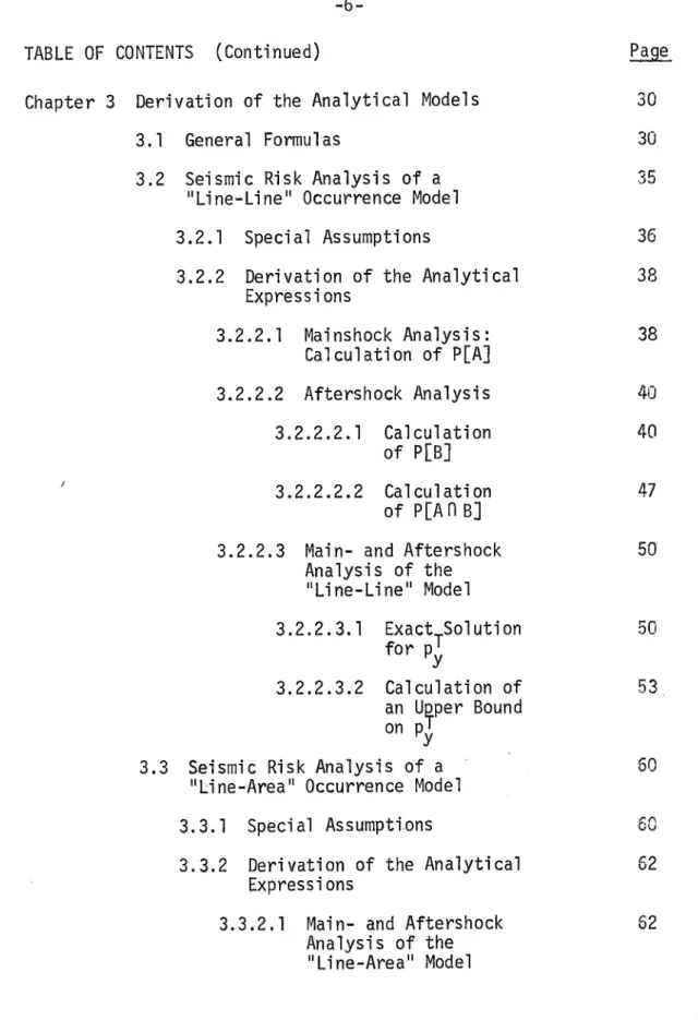
The "line-line" occurrence model is defined by the assumption that both the mainshock and the aftershock epicenters lie on the same fault line, i.e., that an earthquake source can be reduced to a line. This assumption clearly contradicts the observed two-dimensional scattering of aftershock epicenters around the main-shock epicenters, that was discussed in Section 2.4.2. However, it is the simplest model that retains the spatial distribution of aftershocks and it simplifies the analytical expressions, es-pecially those for the estimate of an upper bound on the risk. A typical fault-site configuration of this model and a typical main-shock with its aftermain-shocks are shown in Figure 3-1. As mentioned

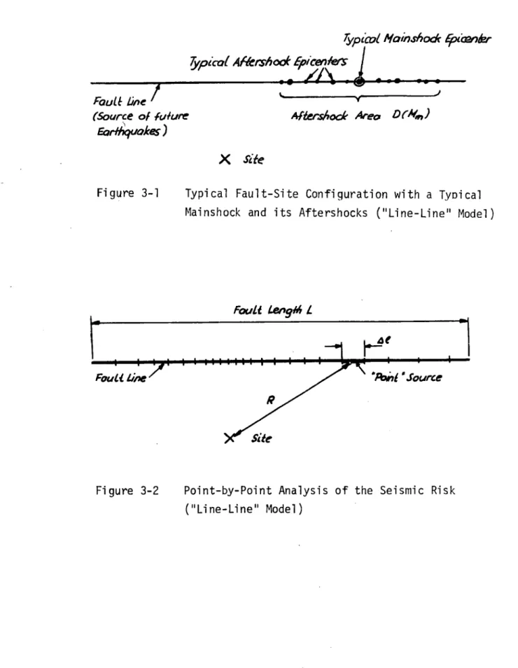
above, this "line source" will be represented in this analysis as a set of many "point" sources (see Figure 3-2).

3.2.1 Special Assumptions

With the exception of the spatial distribution law for

aftershock epicenters (Eq. (6), Section 2.4.2), all the assumptions and parameter relationships of the previous chapter can be used without modifications in this model. Because of the assumption that the aftershock epicenters lie all on the fault line, rather than being scattered in an areal region around the mainshock epi-centers, the spatial distribution law has to be written in a dif-ferent form. Eq. (7) in Section 2.4.2 gives the linear dimension D

(diameter) of the aftershock area as a function of the mainshock magnitude. It seems reasonable to use this relationship of the form

?OY1 Z . 7 '+6'Mm (24)

as the spatial distribution law in the "line-line" model. In addition, it is assumed that in general (exceptions will be given below), the linear aftershock region D extends D/2 on both sides of the mainshock epicenter. This implies that a mainshock with magnitude Mm can potentially produce an aftershock in a "point" source on the fault if it occurs within a region of D(M m)/2 on either side of the "point" source.

-37-ypicol Mainshodc iptbAc r 5ypico( Afthoot Fpicee/

Fault Line (Source of Miure Earl/qakes) Fi gure 3-1

T

site

ypical Fault-Site Configuration with a Typi cal ainshock and its Aftershocks ("Line-Line" Model)

Foli lenqgi L

Site

Figure 3-2 Point-by-Point Analysis of the Seismic Risk ("Line-Line" Model)

3.2.2 Derivation of the Analytical Expressions

3.2.2.1 Mainshock Analysis: Calculation of P[A]

Given a mainshock occurs in a "point" source (see Figure 3-2) with distance R to the site, the probability p that the_m

seismic intensity at the site will exceed y is given by (Cornell(') formula (13))*

Pyse

>Y]

j,=.

(<

kM)

0e(O)

e

esm.

= b - ln 10 = constant of the magnitude frequency law (Section 2.2) b_{1, b2, b}

3, a

km

(Im

ml m

e

are the constants in the attenuation law (Section 2.5)

-,~(m~(26)

are an upper and lower bound on

the mainshock magnitude (Section 2.2)

* A formula for the same probability using a quadratic instead of a linear magnitude-frequency law, as proposed by Shlien and

Toksoz(1 4), has been derived by Merz and Cornell(8). In addition, it is shown there .that it is possible to use a partly linear, partly quadratic magnitUde-frequency law.

+

)

(y/4)

R

r9/

-39-z

eny

- en

(

",

complementary cumulative distribution function of the standardized Gaussian distribution.

If Vm denotes the mean number of mainshock events per year with magnitudes larger than a lower bound m occurring on the entire

*0

fault of length L, then the expected number of events in T years E[nm T] is given by

E[nm

j=vmT

If it is equally likely for a mainshock to occur anywhere on the fault line, the expected number of events with magnitudes larger than mm occurring in the "point" source of length At during T years

0 is given by

V

T^-

_Lny

E [nm

e-A

L

Therefore, the expected number of mainshocks in AP during T years producing a seismic intensity at the site in excess of y is

Thus, the total expected number of mainshocks Einm T] on the fault during T years, which produce ysite > y, can be written as

E[rn>]=

Efnm

71

'

1

PA]=1

-expVmTZ]

In order to give the expression for P[B], the

proba-bility Ceter* has to be calculated,

(see Eq. (21)). Given the mainshock in question occurs at time t' to t' + dt' during T in a particular "point" source of At and has a magnitude between mm and mm + dmm, the total expected number of aftershocks, E[hra], with magnitudes larger than a lower bound m a during t' and T-(T and t' in years) is given through the modi-fied Omori law (Section 2.1.2) as

rr

E[na]

vO.

(365(e'-

0)6

d'

36(V"

4')+c

5d

S"

S(35T-)

')

c}k'-c

O i

.

T

-41-where A is given by Eq. (2) in Section 2.1.2. The factor 365 is the average number of days per year and is necessary because the modified Omori law gives the aftershock frequency per day. Clearly, Eq. (33) is valid only for p 1.

The size of the aftershock region D(m ) is given by the spatial_m distribution law (Eq. (24)). If this region is divided into inter-vals -of lengths A~i for which fixed distances to the site can be assumed, the expected number of aftershocks in any particular interval is, with the equally likely assumption for the location of aftershocks

E[naj

i

L

From these aftershocks of magnitudes above m a, only a fraction will 0

produce a seismic intensity at-the site in excess of y, namely

E[nao

where is the probability that, given an aftershock occurs in Ak,., the seismic intensity at the site will exceed y. The-proba-bility p is analogous to Eq. (25) given by

[a

)

where mm is the upper bound on the aftershock magnitude which is equal to the magnitude of the causative mainshock

(Section 2.2)

ma is the lower bound on the aftershock 0 magnitude (m < mni for reasons to

be given later)

- (37)

2

=

ny

-

en

(be

"'"

AD

)

and the other parameters are equal to the ones described in Eq. (25).

Analogous to the step from Eq. (30) to Eq. (31) in the main-shock analysis, the total expected number of aftermain-shocks during t' to T which produce ysite > y, due to a mainshock of magnitude .mm at time t' in the "point" source A9, can be written as

E[

a]o-

-6m

)

-43-Thus, the probability that at least one aftershock occurs during t' to T and causes ysite > _{y, given a mainshock of magnitude mm} occurs at time t' in "point"source Az, _{is (Poisson process)I}

exfErna]

7

The probability that the mainshock occurs in the "point" source AP, is given by AZ/L (see Eq. 29). Because, given one occurs, it is equally likely for a mainshock to occur at any time during T, the probability that it occurs durin" t' to t' + dt' is simply dt'/T. The truncated magnitude-frequency law for mainshocks

(Eq. (4), Section 2.3) implies a probability density function over the magnitudes of

4M,

(Mm)

(4

where

(42)

S()(43)

Now, the probability that at least one aftershock occurs during t' to T and causes ysite > y, due to a mainshock at t' to t' + dt' in a "point" source of length A* and of magnitude between mm and mm + dmm, can be given by

[1-expj-E[nca]

D

₎

(44) In order to account for all possible times t', and all pos-sible mainshock magnitudes mm as well as all pospos-sible locations At, Eq. (44) has to be integrated over t' from t' = 0 to t' = T and over mm from mm = mm to M M and finally summed over all Ak on the fault line. Thus,

7 m, a Oa 0 m," Mali C - C tP 41

C)

c

,4

dmm.

a' I

QsV

where km is given by Eq. (26) 1 g A is given by Eq. (36) A is given by Eq. (2) D(m ) is given by Eq. (24) m

-45-Pe] =1-

exp

tE7nm']P

e(/(MM MOM'

)'

~1~ep

f-eL

mm

₁

7 r

Qn~ea'nd 4e

The integration over the mainshock magnitudes from m to m implies that only aftershock sequences of mainshocks with magni-tudes between these limits are considered. However, the lower limit mm can be chosen arbitrarily, as long as at the same time the condition ma < Mm is satisfied. The necessary adjustments in

0 0

the other parameters are carried out automatically.* The reason

* If the lower bound is changed from mm to mo , on one hand the mean rate of occurrence vm has to be cnanged by a factor

J 0(m m')

and on the other hand, the probability density function over the magnitudes changes by a factor of

O - m3')

for the condition ma < mi is that Eq. (36) for p and the

under-0 0a

a =M* lying parameter relationships are not valid for the case m = m 0.

However, the difference between mm and ma can be small, say 0.1

0 0

magnitudes.

A special situation arises for "point" sources located near the end of the fault line where the distance from the "point" source to the end of the fault line is smaller than D(m m)/2, where

D(m m) is the potential aftershock region associated with a main-shock of magnitude mm. In this case, the assumptions that all

aftershock epicenters lie on the fault line and that the region of potential aftershock epicenters extends D(m m)/2 on either side of the mainshock epicenter are no longer compatible. This problem emerges essentially from the problem of defining the beginning or the end of a fault-line, and, at this time, there is no way of solving it completely and satisfactorily. In any case, either one of the two assumptions has to be given up. For instance, it is possible to maintain the size of the aftershock region but allow near the end of the fault-line that the mainshock epicenters are no longer the center of the region. This approach implies a con-centration of aftershocks in the end regions of a fault-line. In cases where the site lies close to one of the defined endpoints of the fault and the concentration of the aftershocks near the

end-* For m = mm the factor kmm (Eq. (37)) in the cumulative distri-bution function of the aftershock magnitudes goes to infinity. The reason is that in this case the magnitude-frequency law of the form logio n = a - bma is not valid, but is reduced to a single point.

-47-points is believed to be wrong, it--i-s suggested that the equally likely assumption for the location of the mainshocks along the fault (Section 2.4.1) be abolished and the end of a fault line be defined by a diminishing probability of mainshock occurrences in this region. With this method, a fault line can theoretically be extended to infinity and Eq. (46) for P[B] can be applied without changes.

Under the equally likely assumption for the occurrence of. mainshocks on the fault, it is a necessary condition that the

length L of a fault line is equal or larger than the linear dimen-sion of the aftershock region for the largest possible mainshock (magnitude _m )

L >

D(Mr,= e

fn 0

"mj)

This condition reflects the statement by seismologists that the length of a fault is correlated with the maximum size of the earthquake magnitudes.

3.2.2.2.2 Calculation of P[AflB]

In order to give the expression for P[A n B], the proba-b iE1fi / texacalv on 1,,7r1.-6c occulrs)

bility

Pn7/-(

The knowledge that the mainshock in question caused ysite > y changes only the probability density function (p.d.f.) over the mainshock magnitudes in each of the individual "point" sources AZ, because the larger the distance R from the mainshock location to

the site, the more likely it is now that- a mainshock of a larger magnitude occurred. In contrast -to Sections 3.2.2.1 and 3.2.2.2.1, where the same p.d.f. over the mainshock magnitude (Eq, (41)) has been applied to all the "point" sources, now, each of these "p6nt"

sources has its individual p.d.f. Thus, once the expression for the new p.d.f.'s has been found, the expression for

1 [P

('

is obtained from

P[8/"(Eq.

by simply replacing the p.d.f. over the mainshock magnitudes. Given the mainshock which produced y site> y occurs in a particular "point" source with distance R to the site, the proba-bility that its magnitude lay between mm and mm + dmm can be written with Bayes' Theorem as

P[m rn4

M

dm

/y,,

>y]=

>'I(4 O

where <mMe

k/

(see Eq. (41)). (49)

P reti >1

IE.

(see Eq. (25)) (50)

-49-P[y>y/(

0,

<m,+d~m,,)]-

E

>

(ny

-$?$$ ( 51 )

where R = -distance from "point" source to the site

z =lny- ln(b1 ebm R

)

= complementary cumulative distribution function of the standardized Gaussian distribution

Thus, the new p.d.f. over the mainshock magnitude in a "point" source with distance R to the site can be written as

,, ) eI72, (53)

PMe

Replacing the "old" p.d.f. (Eq. (41)) it -Eq. (45) 6y the "new p.d.f. (Eq. (53)) yields

Cou >

1h raeU's 0 -.

where k m A D(mm -i is is is is is is given given given gi ven given given by by by by by by Eq. Eq. Eq. Eq. Eq. Eq. (52) (25) (26) (2) (24) (36)

The expression for P[An B] is therefore (see Eq. (22) and (31))

7A3]

exp

f-

E[nmy'P[B(2*'

Yse;Y

17-(55)

The same remarks with respect to "point" sources located near the end of the fault line and to the condition mm > m , and with

respect to the maximum magnitude and the length of the fault line, made at the end of Section 3.2.2.2.1 apply here as well.

3.2.2.3 Main- and Aftershock Analysis of the "Line-Line" Model

3.2.2.3.1 Exact Solution for pT Py

-51-and P[An B] (Eq. (55)), the desired probabilityp that at least one mainshock or at least one aftershock occurs in T years and causes a seismic intensity at the site in excess of y, can now be given as

p=

P[A]+P[J-P[AOB]

-I

x;

faea

-exp

L-

L

e

6'""''"d9-exp

sr-1L

di'j

where Pm is given by Eq. (25) pa is given by Eq. (36) km is given by Eq. (26) A is given by Eq. (2) D(m ) is given by Eq. (24) z' is given by Eq.. (38)

*(-) = complementary cumulative distribution function of the standardized Gaussian distribution

Eq. (56) gives the probability that at least one main- or after-shock produces a maximum peak seismic intensity in excess of y

T

in T years. For small risks (say py < 0.1) an "average annual" probability p1 can be obtained by dividing p by T

y y

(57)

So far, nothing has been said about criteria for the choice of the size At of the individual "point" sources. Unlike the

"line-area" model to follow, the lengths At are governed only by the assumption of fixed distances to the site. If, for instance, the parameter b3 in the attenuation "law" (Eq. (8), Section 2.5) is 2.G, a variation of the distance R by 5% will change the risks by approximately 10%. A reasonable rule for the determination of At is that the distance should not vary more than 1% when going from one endpoint of the "point" source to the other, for "point"

-53-sources near the site, and not more than 2 to 5% for more distant "point" sources.

Because the double integral over the time and mainshock epi-centers can neither be separated nor solved analytically, it has t be evaluated numerically. In addition, the values of P[B] and P[AflB] can be very close in many cases, which requires precision in evaluating the terms. The numerical evaluation of Eq. (56) for p T is therefore very complicated and time consuming. In the

y

following section a method to calculate an upper bound on pyT will be presented.

3.2.2.3.2 Calculation of an Upper Bound on pyT

Compared with the computations necessary to obtain the "exact" value of p from Eq. (56) in the previous section, it is

y

T

relatively easy to calculate an upper bound on p y, which is still a significant improvement over the present upper bound ("equivalent event" model, see Chapter 1).

An upper bound on p T is obtained if in the equation of p

y y

(Eq. (11), Section 3.1)

oj

=

1P[A]+

P[B]- P[A

B]

the term P[A fB] is omitted and if P[B] (Eq. (46)) is approximatec by

where E[na _y] is the total expected number of aftershocks in T years which produce a seismic intensity at the site in excess of y. De-tails about this approximation are given at the end of this section. With Eq. (58) it is assumed that aftershocks are marginally governed by a Poisson process. Especially for small values of y, this is a very bad assumption, because the aftershocks cannot be considered as totally independent of each other at these low levels of y. For higher values of y, however, the Poisson assumption becomes more reasonable. As it will be shown in the following, this approxima-tion greatly simplifies the analytical expressions and their nu-merical evaluation.

The expected number E[naT ] can be written as (see also Eq. (19), y

(20), (21))

0* _{n -Ei '}

Efno|]

2

nE[1a/

(Ec

"t

ar|f r

1.7

or

E[noj]

E[rm7

[nOf/(e

where E[nmTI is defined as the total expected number of mainshocks with. magnitudes above m0 and giveh by Eq. (28). (Section 3.2.2.1) as

E-jnMr7 r

'

7

Given a mainshock of magnitude between mm and mm + dmm occurs at time t' to t' + dt' (0 < t' < T), the expected number of aftershocks