by
Thomas M. Stoker
Massachusetts Institute of Technology November 1980
This paper studies the aggregation structure necessary for several common assumptions on macroeconomic functions to be valid. Sufficient conditions are found for linearity of a macro function, including linear functional form (LFF) and linear probability movement (LPM) structures. Necessary and sufficient conditions are found for omitting a distribution
parameter from a macro function. These conditions often provide testable covariance restrictions when the distribution form is known. For the case of unknown distribution form, necessary and sufficient conditions are found for a macro function to depend only on a predictor variable mean, on marginal distributions of jointly distributed variables, and on overall means when the predictor distribution is segmented. A simple model is presented to analyze changing domain of predictor variables. Finally, issues of interpreting and constructing macroeconomic functions are discussed.
KEY WORDS
Aggregation Theory Linear Functional Form Linear Probability Movement
Massachusetts Institute of Technology, Cambridge, MA, 02139. The author wishes to thank Zvi Griliches for early discussion of this topic, and Julio Rotemberg for several helpful discussions.
1. INTRODUCTION
When formulating macroeconomic modelsl of average data, economists usually have a theory pertaining only to the behavior of a rational individual. If a model based on individual behavior is directly implemented with average data, the researcher implicitly makes a number of strong assumptions about the distributional influences on the average data. For example, suppose that a theory states that consumption is an increasing function of disposable income for each individual in the population. If the researcher then regresses
average consumption on average disposable income, he has assumed first that all changes in the disposable income distribution (other than the average) are
irrelevant to average consumption, and second that the true relation between average consumption and average disposable income is linear. Failure of either of these assumptions removes any structural or behavioral interpretation of the results of the regression.3
In general the movement of an average dependent variable depends on both the true behavioral relationship for individuals and all changing parameters of the predictor variable distribution. In the above example, average
con-sumption will usually depend not only on average income, but also any other changing income distribution parameter, such as the variance, skewness, and
(if the elderly save differently than others) the percentage of income accounted for by the elderly. Consequently, correctly modeling an average-dependent
variable not only requires knowledge of the individual behavioral relation, but may also require a large amount of detailed information on the underlying distribution movement.
Frequently assumptions are made which allow a macro function to be written in a simplified form. Typically, these assumptions allow all distribution
parameters other than predictor means to be omitted from the aggregate formulation. Also, common assumptions allow the basic structural macro model to be written in
linear form.
There are several reasons why such simplifying assumptions are either con-venient or necessary to use. First, the vast majority of statistical techniques available for estimation and testing of macroeconomic models rely on a linear structural form as their foundation. Second, even if the predictor variable
distribution is observed for all time periods under study, it may be computationally infeasible (or too costly) to capture all of the observed detail in the average variable analysis.4 Alternatively, and usually the case, only partial aspects of the distribution are observed, requiring a simplified aggregate model by necessity.
The purpose of this paper is to establish the structure which underlies several common simplifying assumptions made on macroeconomic relations. This study requires a direct investigation of the interaction between the individual behavioral relation and the movement of the predictor variable distribution through the process of aggregation. Each simplifying assumption generally involves restrictions on the individual relationship between the dependent and independent variables, restrictions on the movement of the independent variable distribution, or a combination of both.
For example, to insure that average consumption depends only on average income, one could assume that consumption is a linear function of income for every individual, with coefficients constant across individuals. Average
consumption is then the same linear function of average income. Restrictions
5
of this type are the focus of linear aggregation theory, and allow such simplified aggregate functions for arbitrary movements in the underlying distribution.
Alternatively, there are situations where the distribution movement is restricted, making linearity assumptions as above unnecessarily strong. If movements in the income distribution are completely parameterized by mean
income, then average consumption depends only on mean income regardless of the individual consumption-income relationship.6
The above discussion points out two types of assumptions which guarantee a particular form of macro function. The existing literature on aggregation in economics7 essentially provides several sets of sufficient conditions such as those above. Here, through a general formulation, we study the precise
structure underlying all such sets of sufficient conditions.
After presenting the notation and formally stating the problem, we begin the exposition by discussing the types of assumptions which guarantee a linear aggregate function. We next turn to the general conditions allowing parameters to be omitted from aggregate functions. Here the first aspect discussed is the conditions allowing a particular parameter to be omitted when the distri-bution form is known; and illustrated by applying them to distridistri-butions of the exponential family. The second aspect discussed is the conditions under which the aggregate function depends only on certain parameters with the distribution form unknown. This problem is technically quite complex, and so characterizing theorems are shown for discrete distributions only, which allow easier inter-pretation.
These theorems are then applied to three classes of problems, picked for their practical applicability. First is the problem of when the aggregate function depends only on the mean of the predictor variable distribution. This
is clearly the most prevalent assumption in empirical studies of aggregate relationships. After applying the general theorems, several examples are
to focus on the linearity of the aggregate function in the predictor variable mean. Finally, the structure required for the use of several predictor variable means is seen to generalize the earlier development only slightly.
The second class of problems arises when averaging is performed over the joint distribution of two or more variables. Here the researcher may not
observe the entire joint distribution, but rather only the marginal distribution of each relevant variable. For example, consumption for each individual may depend on both his income and his age, requiring average consumption to depend on the joint distribution of age and income in the population. If data on the marginal distributions of age and of income are all that is available, then a simplified aggregate function is required. We apply the characterization
theorems to this problem, and then illustrate the structure with several examples. We close by discussing when the individual component means may be used in place of the full marginal distributions.
The third problem concerns when segmented distribution information can be ignored. Returning to the case where consumption depends only on income, suppose that average income data for urban consumers and for rural consumers are separately observed, as well as the percentage of rural consumers in the population. When will average consumption depend only on overall average income, allowing the segmented distribution detail to be ignored? We analyze this problem for general distributions, and illustrate the solution by applying the characterization theorems applicable to discrete distributions for this case.
Each of these problems is studied assuming that the domain of the predictor variables does not change over time. We continue the exposition by discussing the modifications of our analysis induced by a changing domain, and present a simple model to study these modifications. This model is then applied to the simplest form of domain movement, namely through translation and scaling.
We conclude with a summary of our results and a discussion of their potential uses. Our results not only generalize all previous studies of aggregation in economics, but also indicate problems in interpreting estimated macro relations, plus the correct structures to assume and test in the con-struction of macroeconomic models.
2. NOTATION
We begin by setting up the basic notation required for our study. For each time period and each individual agent, there is a dependent quantity of
interest x determined by an underlying variable A through an individual be-havioral function x = x(A). We assume that A captures all relevant differ-ences across agents, so that the function x = x(A) may be assumed identical across individual agents and time periods. In addition, A is assumed to be a scalar variable for simplicity, and we will consider several predictor variables when the need arises.
In each time period, we assume that the quantity A for each agent repre-sents a random drawing from a distribution with density p(Aie). e is a vector of parameters indicating how the distribution changes over time periods. We assume that the number of agents i the economy is large, so that average variables can be associated with their population expectations.9 Consequently the average of x, denoted p(O), is written as
+(e) = E(x) = /x(A)p(Ae)dA (2.1)
E(x) = (e) is the true macro relation connecting average x to the changing distribution parameters . In the consumption-income example, x represents consumption, A income and p(Aje) the income distribution. 0 can have as components mean income, the variance of income, and any other changing distri-butional parameter such as skewness or kurtosis.
For general forms of the distribution p(Ae0) and the behavioral function x(A), the form of (e) can be arbitrary, depending on all components of the vector 0. Our primary interest in this paper are the conditions under which
p(e)
can be simplified, either to a function linear in the components of 0, or by allowing certain components of e to be omitted from (e).Before discussing linearity of (0O), three points require mention. The first is the role of time. While not explicitly included in the notation, time is a crucial element in the interpretation of . With a given function x(A), the function (e) is determined entirely by p(Ale) which changes only through the parameter . Thus a could be denoted with a time subscript, which, while unnecessary for the formulae to follow, would remind the reader of this
interpretation. Also note that nothing is said of the particular value of A for any agent in any time period. All that is required to determine (0) is p(Afe), and thus particular agents can interchange positions randomly over time periods.
The second point regards the constancy of the function x(A). While A captures all relevant differences across agents in any one time period, there maybe common parameters, such as prices, which change the form of x(A)
over time. While these parameters could easily be incorporated in the form of x(A),10 they are unnecessary for considering the distributional effects
on E(x) = (e), so we omit them for simplicity.
Finally, note that the formulation (2.1) of (e) assumes a constant domain for the variable A,l l with e acting only on the density p(Ale). This is
crucial to the results of Sections 3-4.4, and while some of the required modifications are indicated in Section 5, the general solutions for varying
domain are relegated to future research.
3. LINEAR AGGREGATE FUNCTIONS
In this section we consider e to be a single scalar parameter, and establish sufficient conditions for E(x) = (e) = a + be, with a and b
constant coefficients over time. This presentation is designed to illustrate both assumptions on the form of x(A) and the form of p(Aie), which will appear
___~~~~~_~~--frequently in subsequent sections.
If is the mean of A; 0 = E(A), and the behavioral function is linear in A, i.e. x(A) = a + bA, then clearly the macro function is linear in , via (e) = E(x) = a + bE(A) = a + be. This structure on x(A) is referred to as a linear functional form (LFF), and guarantees a linear aggregate function
for all forms of the density p(Ale).12
In order to discover other conditions guaranteeing ~(0) = a + be, note that a necessary and sufficient condition is that the second derivative of C vanishes.13 Assuming p to be twice differentiable in and that derivatives may be passed under the integral sign, this condition appears as:
2 2=
0 = - - jx(A)
e
2 dA (3.1)A second set of conditions guaranteeing the linearity of are when 2 =
ae2
for all A. This implies that p(Ale) can be written as:
P(Ale) = l(A) + P2(A) (3.2)
where Pi and P2 do not depend on . Since f p(Ae)dA = 1 for all ;
f
P1(A)dA + fp2(A)dA = 1 for all , which implies f P(A)dA = I andf p2(A)dA = 0. Consequently pi(A) represents a base density, 14 and p2(A) a distribution shift, occurring linearly with respect to . The structure
(3.2) is referred to as linear probability movement (LPM), and represents movement of p(Ale) over time by simple extrapolation with respect to 0. c(0)
in this case is:
f(e) = fx(A)pl(A)dA + 0 fx(A)p2(A)dA
= a + b
x = x(A), and thus LPM represents the "opposite" of LFF, which insures linearity for all distribution forms.
Any combination x(A), p(AIe) obeying condition (3.1) will produce a linear macro function . For example. suppose that p3(A) is any function orthogonal to x(A); i.e. Ix(A)p3(A)dA = O. Then
p(AJO) = p(e) + p2(A) + d(e)p3(A) (3.3) is a density15 whose movement insures a linear macro function. Viewing
(3.3) from the standpoint of a fixed function p3(A), a linear macro function is guaranteed for any behavioral function x(A) orthogonal to p3(A). This interdependence of distribution and functional form is typical of the problems studied here, and reappears in future sections.
Notice in addition that if is a K-vector of several parameters, a multi-variate version of LPM can be defined, with p(Ale) moving over time by a
linear combination of K shift functions. Similarly if represents the means of K underlying variables, a corresponding form of LFF is defined hrough x being a linear function of these underlying variables. Either LPM or LFF in this form guarantees an aggregate function (0) linear in the components of .
We now turn to a discussion of omitting components of e from E(x) = ¢(0).
4. OMITTING PARAMETERS
We begin our discussion of omitting parameters from E(x) =
q(o)
with a general development and then turn to the specific problems mentioned in theintroduction. e is a K vector, here partitioned as = (00,e1), where O is a K vector and 01 a K1 > O vector, KO + K1 = K. Our interest is in the
conditions under which E(x) is a function of O0 only; i.e. (e) appears as: 4(e) = fx(A)p(A e)dA= =O(eO)
where 0O does not depend on 1.
This property is clearly guaranteed if p(AIG) depends only on 0, or if there exists a functional relation 1 = g(80) between 81 and 00 for all time periods. To remove these uninteresting cases from our analysis, we adopt:
Assumption 1: 0 = {8 RK p(Ale) is a density} has a nonempty
ineir K 1 1 1)
interior in IRK. Also, there exists = ( 0,0I) and
2 22 1 2 1 2
2 = (00,61), , 0 such that 1 1 and p(AI ) p(A!02) for all A.
For our discussion of general forms x(A) and densities p(A|I),16 we must also adopt:
Assumption 2: () and p(Ae) are differentiable in the components of e1 for all A and e O and differentiation may be performed under the integral defining (8e).
Now, under assumptions 1 and 2, 01 can be omitted from E(x) = (8) if and only if the gradient V 1 vanishes for all e O. This gradient can be expressed
in the following two equivalent ways:
0 = Vx(
=
A p(A)(Ae)dA (4.la)= Cov(x(A),VO ln p) (4.lb)
where the latter equality follows from E(Ve In p) = O. Equation (4.la) states that x(A) must be orthogonal to each component of V p via the integral inner product. This version is useful in our later analysis, where the density p is orthogonally decomposed and 80 and 1 related to the decomposition. Equation
(4.lb) states that x(A) and each component of the score vector Ve ln p are uncorrelated. This form is useful when the form of the density p is known, as
Example 1:
Suppose that p is a member of the exponential family in its natural parameter izat ion:17
p
=:C(,r)h(A)exp
(
n.v.(A)
i=l I I
where
Tr=(
i,...,
K) is a vector of parameters and v = (vl(A),...,vK(A)) is
a vector function of A. Let 6 = with 0 = (1'' ' K-1) and 60 = TK. Then E(x) = (W) does not depend on K if and only if0 = Cov (x(A), aln P)
= Cov (x(A), lnC( + vK(A))
K
= Cov (x(A), vK(A))
i.e. x(A) and vK(A) are uncorrelated for all = 0E6.
Example 2:
Suppose that p is a member of the exponential family as above. From a practical point of view, it is more interesting to inquire when E(x) is
determined by the means of v(A), i = 1, ... , K-l, omitting the mean of vK(A). Denoting as = ('...*'K)' the vector of means (i = E(vi(A)), i=l,...,K) we reparameterize the density p with respect to , and set = , with 00 = ( " 'PK-1)'
e1
= K' It can be shown that the gradient of with respect to the full vector is18Ve+ = E((v-v)(v-p)')E((x-+(e))(v-p))
the vector of "slope regression coefficients." Thus 61 = K can be omitted from E(x) = (e) if and only if its associated regression coefficient is zero.
Example 3:
Suppose that p is a normal density with mean and variance a 2 Our
2 2
interest is in when a can be omitted from E(x), so let = (,a 2),
i0
= ,2 2
~1 = a . Since In p = - In 2 - In 2 - 2
Cov 9o22
22 o-= Cov (x(A-~) )
Thus E(x) depends only on 60 = p if and only if x(A) is uncorrelated with the squared derivation (A-p)2 forall ,a2 . Unfortunately this is all that can be said in general. If x(A) is linear in A, then clearly this covariance vanishes:
let x(A) = a + bA, then
Cov((a+bA),(A-p) ) = bE((A-p) 3) = O
2
for all ,a . Also, as can be easily verified, if x(A) is quadratic in A, then it is impossible to omit a2 from E(x).
In each of these examples, equation (4.lb) was used to obtain conditions requiring a specific covariance to vanish for all 0OE. With cross-section data for a single time period, these covariances can be estimated consistently, and thus the condition that they vanish tested. Consequently, when the density
form p is known or assumed, the conditions for omitting parameters can be tested, with rejection of such conditions indicating that the respective distribution parameters must be included.19
While (4.1lb) is a valid condition for all problems of omitting parameters, it is less useful than (4.la) for analyzing assumptions that E(x) = (e) depends
only on certain distribution aspects (such as independent variable means) for all possible distributions. For this case, the orthogonality indicated by
(4.la) provides a useful focus. The analysis of this problem for discrete densities follows.
4.1 Parameter Omission with Discrete Distributions
This problem is best addressed by considering the density p(AIe) and the function x(A) as vectors. Suppose that there are N possible types of agents, indexed by i = 1, ..., N, with the i type occurring in the population with probability (or proportion ) pi(e). The vector of probabilities is denoted p(e) = (pl(e),..,pN( ))' and lies in the unit simplex T = pe RN ip = 1, p >, 0 } where i = (1,...,1)'.
Any random variable taking values for the N possible consumer types can be represented by an N vector. Denote by A = (Al,..., A N)' the independent quantity of interest, and by x = (x(A1),...,x(AN))' the dependent quantity.
Expectations appear simply as inner products:
E(A) = A'p(e)
and E(x) = x'p(e) = (e)
Our general strategy in studying parameter omission will be to express the movement of p(e) in T in terms of N-l orthogonal directions. These directions are then related to the parameter subvectors 80 and 1. We begin by noting that
N
p(e) = pi(e)ei i (4.2)
i=1
where e. = (0,...,1...,0)' is the th unit vector of RN e
N 21 /
represents an orthogonal basis of R , with pi(a) the coefficient of e.. In order to guarantee that i'p(e) = 1, we choose N-1 vectors 6, i = 2, ... , N,
I
such that {i',2'...' N is an orthogonal basis of R (4.2) above can be written uniquely as: N
p(6) = i + Z d.(e) 6 (4.3)
i=2
where d.(e), i = 2, ..., N are the transformed coefficients from (4.2). Since i'6. = 0, i = 2, ..., N , the second term of (4.3) represents the movement of p(e) in the unit simplex T, with 62,...,' N the orthogonal
directions of movement and d(e) gauging the amount of movement in direction i.22 Recall that = (60'61)' and that our interest is in determining when
E(x) = (e) = (0). For this purpose the decomposition (4.3) must be altered to be minimal in 1 in the following sense.
Theorem 1: Given Assumption 1, there exists a decomposition of p:
N1 N2
P(e) = 1 + Z f (e ) + Z gj(e 0,o 1)
i-=l i j=1 1
where i, 6., i = 1, ...N ,j, j = 1, ...N2 are
ortho-gonal vectors and N1 + N2 < N-l, such that if
Eaj9j(001e) = f(6 0) then a = 0 for j = 1, ..., N2.
Such a decomposition is called minimal in 1. Moreover, given any other decomposition which is minimal in 1, say
N I' N2 **
p(6) = i+ f: (6 )6+ z g. (O6el )
N -i=l j=1
then N2 = N2, and 23
SPAN 1 · 2 = SPAN 2
Proof: See the Appendix.
Proof: See the Appendix.
The implication of this theorem is that the action of 1 on p(e) can be isolated to a unique subspace of directions S = SPAN { ~I' N '''. The result allowing use of this decomposition is:
Theorem 2: Let xE RN represent a random variable x. E(x) = 0(00)
1 1
if and only if xS , where S - in the subspace
ortho-01 1
gonal to S in RN.
Proof: See the Appendix.
When discussing several parameterizations of a given density, another useful property is given by:
Theorem 3: Suppose that 01 and 01' are K1 vectors of parameters, and there exists a function 01 = g(01) which is - 1. Then if p(e) is reparameterized to '(0'), with
' (0,eO ') then S S 1 Proof: See the Appendix.
Thus, a 1-1 reparameterization of p holding 80 constant does not alter the subspace of contaminated directions Se.
This machinery allows us to analyze the substantive problems raised in the Introduction.
4.2 Aggregate Functions Depending only on Predictor Variable Means
In our basic setup, A is a scalar variable whose mean we denote by P. Recall that
v = A'p(0) (4.4)
where A is the vector representing A and p(e) is the vector of probabilities. 24
For this problem we assume that 0 = (p,01), and consider the conditions under which E(x) = 0(p).M
We study this problem by finding a unique direction vector A associated
with for all density vectors obeying (4.4). A is found by orthogonally decomposing A as:
A : Ai + (A -
Ti)
=Ai + AN
with A = Z A./N, the (unweighted) average of possible values of A. Now,
i=l1
for any density vector p(P, 1), choose N-2 vectors i ,.., such that {i, A, 3 . , is an orthogonal basis of R , and write p(p,01) as:
N
P1 D*(, )A + d (4,5)
p~vi,0) 1 - 1
_ -1~ N 1 i=3
where D* and d., i = 3, ..., N represent the relevant coefficients. That A is a unique direction associated with is shown via (4.4) and (4.5) as:
=
Ap(, 1) =N Ai'i + D (,el ) A'A
= A + D*(,e01) A'A so
D*(,61) = (vi-A)/A'A = D()
Thus D (,0 1) = D(p) depends only on p in a linear way. Note that the form of D(V) is the same for all density vectors obeying (4.4). Finally, from Theorem 1, write (4.5) in minimal form as:
N1 N2
) = i + D(p)A + f (Pi) + i (4.6)
l-i=2 j=l '
1-where N1 + N2 < N - 1.
Before presenting the main result of this section, recall that the function x(A) is represented by an N vector x. x can be written uniquely as:
x = x i + bA + C (4.7)
N25
where x = X x(A.)/N and H'i = A .
i= --
The main result of this section is:
Theorem 4: Given Assumption 1, if p(u,e1) is in the minimal form (4.6) and x is of the form (4.7), then E(x) = x'p(P,6l) =
b0 (p) if and only if 'j = O, j = 1, ..., N2
Corollary 5:
(a) If E(x) = 0O(p) for all distributions obeying E(A) = t, then x(A) = a + bA, where a and b are constants, and
0(p) = a + b.
(b) Any density vector such that E(x) depends only on for all functions x = x(A) must depend only on A, and no other varying parameters.
Proof: Theorem 4 follows directly from Theorem 2. For Corollary 5(a), pick N-2 vectors tE., j = 3, ...-J , N
such that
{
i, A, , ..., Q is an orthogonal basis~~N
~26
of R , and consider the density,
1 N
p(,d3 ...,dN) i + D(pI)A + 2 d..i p( i=3N From Theorem 4, E(x) = 0(v) iff
x= x i + bA = (x - -) i + bA
This is equivalent to the functional form x(A) = a + bA, where a = x - A and b are constants. For (b) suppose that p(,( 1) represents a density such that p depends nontrivially on 01 and E(x) depends only on p for all functions x - x(A). Write p(p,01) in minimal form as:
N1 N2
p(l,1 ) = i + D(ip) A + 2 f.() S. + F gj('el)
If we choose x = 1' then
E(x) = x'p(vi,e) g ( 'l)
which is a contradiction, so we must have
P(v,01) = p(p), depending only on .
Q.E.D. Corollary 5(a) is a refinement of the Fundamental Theorem of Exact
Aggre-gation of Lau (1980), which states that for an aggregate function to depend only on for unrestricted distribution movement, the behavioral function x(A) must be linear in A (i.e. LFF holds). Corollary 5(b) states that if a distribution moves with respect to a parameter other than , then E(x) is a function of v1 only
if x(A) is restricted according to Theorem 4.
We now illustrate the density decomposition and the above theorem with several examples.
Example 4 (N=2):
Assume that A is zero with probability 1-P and one with probability P, so
-1 =
p = (-P,P)', A (0,1)', and = E(A) = P. Here A = A - Ai = A = (-i )
and the decomposition (4.6) appears as
p = Hi + D(P)A
with D(P) = (P-A)/A'A = 2P-1. The direction vector A indicates that p changes only by increasing P and decreasing 1-P simultaneously (or vice versa) in equal amounts. If x(O) = x0 and x(l) = xl, then x = (xO,x1)', and E(x) is a
function of P if x0 # x1, i.e. x(A) is not a constant function, with x collinear with i. Notice in addition that if A was the relevant predictor variable
where A" = (a,b)', a b, then P = E(A ) = a + (b-a)P, and the only changes in the above decomposition would be A = (b-a)A and D*(p) = (2P-a-b)/(b-a)2, with conclusions regarding E(x) unchanged.
Example 5 (N=3):
Let A = (0,1,2)'. If p = (-P-Q,P,Q)' then 1' = E(A) = P + 2Q. Parameterizing p in terms of 0 = (,Q) gives p(P,Q) = (1-1p+Q,Ij-2Q,Q)'. Now T = 1, A = (-1,0,1)', and the decomposition (4.6) of p(p,Q) is
p(l,Q) = i + D(M)A + g(l,Q)
where D(p) = (p--)/A'A = (-1)/2, g(,Q) = Q + and = (,-2,1)'. Here the admissible parameter space is:
O = I{(iQ)Ili,QcR; 0 Q < 1; 2Q << 1 + 2Q}
A corresponds to a precentage shift in probability from the first class to the third, and to a shift from the second class to the first and third (in equal amounts). Now, suppose that a function x = x(A) is represented by a vector x, which in turn can be written as in (4.7):
x = ci + bA + en
E(x) = x'p(vP,Q) is therefore:
1
~E(x) - ci'i + bD(p)A'A + eg(v,Q)
Clearly E(x) is independent of Q iff e = 0, in which case E(x) = (c-b) + bp and x(A) = (c-b) + bA. Any nonlinear function x = x(A) will require E(x) to depend on Q. Also notice that if the movement in p is such that Q is constant, then E(x) is linear in for all possible forms of the function x(A).
To illustrate this example graphically, it is more convenient to use a different parameterization of p, namely
p(p,g) = + D(p) A' + gE
where g = Q + - is now the relevant parametric aspect. The admissible
where g = Q + 6 2
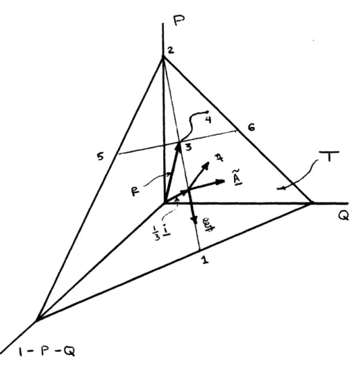
parameter space is now O = (p) ,g) R;- 3 2g9 < + 2g1 The space of possible distributions T is presented in Figure 1. Here the vectcr
i, as well as the directions A and are noted. If g is fixed and = 1, the density vector p lies along segment 12, say at 3. If over time, the density vector moves in a nonlinear way, say along curve 34, then E(x) is a function only of p if x is orthogonal to (i.e. x(A) is linear in A) so that the distance traveled along direction A (i.e. D(p)) solely determines E(x). If g
is constant and varies, the density vector moves along the linear segment 56. In this case, E(x) is a linear function of .
If Q instead of g is held constant, the density vector will move over time along a linear segment parallel to n = A - = (-2,2,0), and E(x) is a (different)
linear function of . Each of these cases corresponds to LPM in , as does movement along any linear segment (except parallel to 12, where is constant),
giving E(x) as a linear function of u.
In this example the role of functional form restrictions (LFF) and distri-bution movement restrictions (LPM) were illustrated as to how they could
insure that E(x) is a (linear) function only of p. The next example considers orthogonality restrictions other than LFF or LPM.
2
G
FIGURE 1: Orthogonal Decomposition when there are Three Types of Individuals (N=3).
__________________ _
Example 6 (N=4):
Let A = (2,4,6,8)'. If p = (-P-Q-R,P,Q,R)'then = E(A) = 2 + 2P + 4Q + 6R. Parameterizing p in terms of e = (,Q,R) gives:
p(i,Q,R) =
2 - + Q + 2R
(
- + -2Q -3R Q
Now A = 5, A = (-3,-1,1,3)' and the decomposition (4.6) appears as:
+ g1(,'Q',R)6 1 + g2(J'Q',R) 62
p(lJ,Q,R) = + D)A
where D(p) = (p-A)/A'A = 204 and 20 4' gl (p,Q,R)61 + 92(vI'Q'R)-2 / / 1- 1 + Q - 2R 3+11 +
-i
- 2Q - 3R 1+ R - 3 2 20with g g2' 61 and 62 to be specified later.
Now, if x = x(A), then E(x) is a function of p if and only
if x(A) is linear in A, with the vector representation x collinear with i and A.
In general if there are N types of consumers, for a given function x(A) there will be N-3 directions in which the density vector can move leaving E(x) unchanged (i.e. the N-3 directions orthogonal to a, A and i of (4.7)). Also,
the N-3 directions are different for different nonlinear functions. We
(4.8)
'x
illustrate this in the current example (N=4, N-3=1) by considering two formulations of x(A).
Suppose first that
x(A) = blA, A < 4
= b2A, A > 4
The reader can verify that x = b + b2, and
x = xi + b12 2] + (b -b2)
where 61 = (-1,2,-1,0)'. E(x) is constant if the density moves in the direction of 62 = (2,-1,-4,3)', which is orthogonal to i,A,61. If (4.8) is written with
61 and 2 above, then we have:
gl(2 + 1 4
91(-iQR) = 3 i R
and 92(p,Q,R) = -- j- + R
From the form of g1, we see that in general E(x) will depend on , Q and R. Also from g1 we see that if the distribution movement is restricted such
4 27
that - AQ = 4AR,2 7 then E(x) is linear in .
As mentioned above, 61 and 62 with the above property vary with changing
2
-functional form. If x(A) = clA + c2A2, then x = 5c1 + 30c2 and
= Xi + ( 1+10c2)A + 4c261
where 6 = (1,- 1,-1,1)'. Orthogonal to i, A and 61 is 62 = (-1,3,-3,1)', and so any distribution movement in the direction of 62 leaves E(x) unchanged. If
(4.8) is written with 61 62 above, we get:
gl(I,Q,R) = - + + R
(Q) 1 1 1 +
92('Q'R) = - - R + 10
The same sort of reasoning can be applied as before, in noting that if density movement is restricted by AQ =- 3R, then E(x) for this case is a linear
function of .
Having illustrated the density decomposition and the interaction of distri-bution movements and functional form structure, we now turn to a discussion of linearity of the aggregate function in . For this purpose, we refine Theorems
1 and 2 to:
Theorem 6: There exists an orthogonal decomposition of p which is minimal in el;
N1 N2 N3
Pl +i + e.(p)0 + + f f + j(P,)+j
N- i=l i k=l k -1 j=l
such that N1 + N2 + N3 < N-1, each e.(p) is a linear function of , and if Z a kfk
(p)
= c + d, then ck = 0k=l
for all k. The subspaces Sn = SPAN{.kt and
Se = SPAN j) are unique for all such decompositions. Moreover, if x represents a function x = x(A), then E(x)
is a linear function of p if
xe (S
S
)
where S
Q
se = SPAN 1'- 'l" 3}See the Appendix. Proof:
Thus E(x) is a linear function of iff x is orthogonal to all directions where either movement of the density is nonlinear in p (via fk()) or dependent upon 1 (via gj(P,'6)). Thus, x must be orthogonal to all directions of move-ment of p except those obeying LPM structure. Each of the constancy conditions referred to in the examples reduced a gj function to one linear in , giving E(x) in each case as a linear function of .
The final topic we address in this section is when there is more than one variable, say A and B, defined over the N possible consumer types. If x = x(A,B), then when can E(x) be written as a function only of A =
E(A) and ~B = E(B)? Here we assume = (PA'B'81) so that e8 = (APB) in the
earlier notation.
The analysis of this case is the same as the previous case with one modi-fication. Let A represent A and B represent B. As before, we define the direction A uniquely associated with A . While a similar direction could be defined for PB$ it would in general not be orthogonal to A. To insure this, we define B as
B =
B
- Bi - r A Nwhere B = E B./N and r = B'A/B'A. i=l
The vectors , A and B are mutually orthogonal.
Now, in order to decompose the density vector p(e) = p(pAPB 1), we choose N-3 vectors 63,... such that ti,A,B,63,. ..,i is an orthogonal basis of
~~~N
R , and write 1NDA(A)
PAPB,1) =I
+ _) + D (PAPBel)B + E di(PAtPB'e1)6i i=3where DA(PA) = (A-A)/A'A from the earlier development. A and B are unique
-I1-_1I-directions associated with lA and 1B, as
B 'P(A'B' 1l) = + rDA(JA) A'A + DB(PAPBl)B'B
= B + r(A-A) + D(!A'B' 1) B'B
so
DB (A'B') (B - B - r( D B(A ,
B'B
Having isolated the dependence of DA and D on only pA and P, B we can proceed as before to consider a minimal decomposition in 01, producing an
invariant subspace S If x represents the function x = x(A,B), then E(x) = O(PA'PB) iffx S0 . We can also show the following result, which is
analogous to Corollary 5: Corollary 7:
(a) If x = x(A,B) is a function such that E(x) = O(IA',B) for all densities obeying pA = E(A) and 1PB = E(B) then x(A) = a + bA + cB, a linear function of A and B, with E(x) = PO(VA'"B) = a +bpA + ctB
(b) If p is a density such that E(x) = O(IpA'B) for all functions x = x (A,B), then p depends only on A and pB.
Proof: (a) and (b) are shown with precisely the same method of proof as in Corollary 5.
For (a), consider the density vector (N>3):
p(PAPB,d3 ....,dN) = + D A + D + DB(AB)B N
+ d.6.
E(x) O(vA'B) omitting d3,...,dN iff
x = xi + b A + c"B
= (+ (rc-b) - c) i + (b*-c*r)A + c B
which corresponds to x(A) = a + bA + cB where a = x + (rc*-b) + c, b = (b*-c*r); c = c are constants (r = B'A/A'A). (b) follows in the same way as Corollary 5(b).
Q.E.D. Clearly these results generalize to the case where there are more than two predictor variables.
This completes our discussion of aggregate functions depending only on predictor variable means.
4.3 Aggregate Functions Depending only on Marginal Distributions
In this section we consider the problem of when an aggregate function depends only on the marginal distributions of the underlying predictor variables, where averaging occurs over the joint distribution of these variables. We analyze this problem for the case of discrete distributions, and our results are primarily all obtained by applying the theorems of the previous section. In order to make the correspondence between this section and the previous one, we require some additional notation.
In this problem A and B are assumed to be jointly distributed random variables. A has N possible (distinct) values A, i = 1, ...,N and B has M possible values Bj,j=l,...,M. The probability of (Ai,B j) is denoted pij(e), where is the vector of parameters determining the joint distribution over time. The marginal distribution of A is given by the probabilities:
_I· I _I
1__1
1_1___1__11_1___111___.
M PROB (A=Ai) = PAi = Z
j=l
and
PROB (A=AN ) = PAN = 1
-N-I
i PAi i=l Similarly the marginal distribution of B is given by:
N PROB (B=Bj)= P Bj = Pij8), i=l PROB (B=BM) = PBM = 1 -M Z PBj j=l
We assume that 0 = (P A .PAN-1' B 'P BM-'0 1) where 1 is a set of oth parameters determining the joint distribution. 01 is assumed nonempty; alth we will later discuss the connection of our results to the case where A and are independent, in which 01 is empty.
Here the behavioral function is x = x(A,B) depending on both predictor variables. The problem we study here is the conditions under which the aggr gate function E(x) = Z pij () x(Ai,Bj) = o(PAAN BM-)
i,j omitting 01 from E(x).
In addition we denote by iN the N vector of ones, by iM the M vector of ones and by i the MN vector of ones. ejM denotes the M vector with 1 in
position j, zeros elsewhere and eiN the N vector with 1 in position i, and zeros elsewhere. The MN vector of probabilities (e) is formed as (0) =
(P1,(e)'P1(0),.''' . M(e)'P21(e),'' PNl(0),'.,pNM(e))'. Now, if we define the following MN vectors
er ough B 2Ai = -iNM ; eBj = N ejM ; j=...,M-1 pi 0 ,ip, . , - e-i=l,...,N-1
we find that
PAi PAi () ; ,..
N-(4.9) PBj =PBj e(e) ;
j=l,...',M-The vectors Ai, i=l,...,N-l and ePBj j=l,...,M-l will play the same role as the vectors A and B of the previous section. There is one major advantage to the structure of PAi and PBi; seen by first orthogonally decomposing them as
* +1 .
P-Ai = Ai + ; i=l,...,N-1
* 1
PBj = Bj + - ;
and showing the following Proposition:
j=l,... ,M-l
Proposition 8: If s E SPAN Ai,.*-AN e 1 and
s
2 E SPAN {B1 '' PBM-1 then 5 's = 0
1 2
Proof: For each i, j, note that
Ai Ai Bj ' (PA Ai-N-N) (PBj )
IPj N Pj M PAi NM1 'i
= Ai Bj -N- Bj M Ai -IM =1-1-1+1=0
Any linear combination of Ai 's is therefore orthogonal to any linear combination of PBj 's
Q.E.D.
The implications of this lemma for orthogonally decomposing p(3) are seen as follows: first define M + N-1 mutually orthogonal vectors i, Al
''' PAN-l' eBI'"'' P-BM- as PA1 = P-A1 -A i *i PAi PA l - E rk i Ak k;i-l i=2,...,N-l = PB1 Bj BjLBj Bj kj- k j-l k jki eBjBj i=2,... ,M-1
where r A Ai'k' Ak)' 5k; = (PBk P'B/BkBk)' and from Lemma 9 there is no need to orthogonalize PBj jl, ...,M-l, with respect to PA To decompose the density, we choose MN - M - N+1 vectors 6k' k = M + N,..., MN, such that
i, A1 ..'AN-I' ,' pB1' -PBM-' ' M+N' "'' MN is an orthogonal
basis of R , and write p(B) as
N-1 M-1 MN
p() : 1i + Z DAi(e)pA + Z DB () PBj + Z d () 6k (4.10)
p(i ) + i=l ai j=l B k=M+N k
Solving out each of the equations in (4.9) yields:
DAi ( 0) = I-- - (PA1-N)
Al Al *1. 1 1 DA (e) = p (PA Ai £ A N Ai Ai = DAi(PAi"'...PA)i) = DAl (PAl)
Z DAkr kAk' Ak) k.i-l (4.11) i=2,...,N-l * _ 1 1
D
Bl"i(e)
=- eI 2 N B1 Bi N and PB1 = DB1 (PB1)DB; (e) 1- (P Z DB S ik '
)
Bj B kj-l Bk Bk
Bj Bj
B=
Bj(PBI' 'PBj) ; j=l,...,M-l
Thus, the coefficient DAi depends only on PA1,...,PA ; the coefficient DBj depends only on PB1 ... PB Thus ,... are directions corresponding
B " BAl AN-I
to the parameters PAl1PP AN-i and ,... , , are directions corresponding
B1 M-1
to the parameters PBl',...PBM_. This is true for all joint distributions with PA1'...,AN--I'AN'PBi PB...,PBM-lPPBM as marginal probabilities. Moreover, as can be checked from (4.11),each DAi and DBj coefficient is linear in its respective arguments.
With this background, we can clearly now proceed as in the previous section, by writing (4.10) in minimal (in 1) form, defining S, and
characterizing the precise structure for a behavioral function x = x(A,B) to allow E(x) = (PAl" O PAN-lPBl...,PBM-l). While this analysis is quite valid, it does not exhibit any particular special properties of the appearance of marginal distributions versus that of several means as the arguments of an aggregate function. The following result exhibits a different form than the previous theorems, but it is actually just a translation of Corollary 7 into the current framework.
Corollary 9: Given Assumption , x = x(A,B) is a function such that E(x) = o(P Ai...l AN-1 PBi,... PBP i) for all joint distributions of A and B with PA1,...,PAN as
the marginal distribution of A and PBi,...,PBM that of B, then x(A,B) = xA(A) + xB(B), i.e. x(A,B) must
be additive in A and B. If x(A,B) is such that
E(x) = (PA1 ... ,PAN-_) for all such distributions, then x(A,B) = xA(A), i.e. x(A,B) depends only on A. Similarly, if E(x) = B(PB ...,P BM-I) for all such distributions, then x(A,B) = xB(B)
Proof: Consider the density vector in the form (4.10) given as
E(PAl' ' ''PAN-I'PB1"' 'PBM-'dM+N'' 'dMN) N-1 M-1 MN- i + " Ai Al' Ai Ai +j- D Bj( B PBBj MN + E dk6 k -k=M+N k
If x is the vector representing x = x(A,B), then
E(x) = o(P ,Al...,AN-l'PBl'" .. BM-i) if and only if:
N-I M-1 x=Xi + g u.e + v. i=l A j=l J-Bj N-l M-1 = ai + Z b p + Y c. P i=l iAi j=l J Bj
where b,i=l,...N-1 are constants arrived at by solving for each in terms of p ,i=l,...,N-, and c., j=l,
Ai Ai J
... , M-1 are arrived at by solving each p in terms Bj
of p ,j=I,...M-1. If we define XA(Ai) = bi,i=l,...,N-l.
Bj
xA(AN) = 0, xB(Bj ) = cj,j=l,...,M-l,xB(BM) = 0, then we have that
x(A,B) = a + xA(A) + XB(B)
and since the constant a may be absorbed in the definition
of xA(A) or xB(B), this can be written as:
x(A,B) = xA(A) + xB(B)
The other statements follow this line of proof exactly.
Q.E.D.
Proposition 8 serves only as a computational advantage for this problem, and does not play a role in the proof of Corollary 9. The appearance of orthogonality between the natural directions for P Aii=l,...,N-l and those of
PBj'j=l,...,M-l, coincides with the property that any function only of A will have an expectation dependent only on PAi,i=l,...,N-l, with the analogous property for functions dependent only on B.
We now illustrate the decomposition structure for joint distributions with two examples.
Example 7 (N=2,M=2):
Let A and B have possible values A = 1, A2 = 0, B1 = 1, B2 = 0. If the joint density vector is written p(e) = (PllP 12'P 21 'P22) then we have PAl = Pll + P12 PB1 = Pll + P21- We reparameterize (e) via PAllPB1 and R Cov(A,B) as 2(PAl'PBl'R) = (PAlPB+R, PA(1-PB1) R,
PB(-P )-R, (1-P Al )(-PB )+R)'. Here p = (1,1,0,0)' ; p = (1,0,1,0)' ;so
Al B]
A1 = 1/2(,1,-1,-1)' ; = 1/2(1,-1,1,-1)'. Now, if 6= 1/4(1,-1,-1,1)'
B1
4
then {i,p , 6} is an orthogonal basis of R , and we write:
2(PAIPB1lR) = i + (PAl-1/2)p + (P81 /2)P
Al BI
+ 4PAlPBl + 4R - 2PA - 2PB + 1)6
E(x) is not dependent on R if x'6 = O. In this case x = xi + u + vl
Al Bl
which corresponds to the behavioral function x(A,B) = a + bA + cB, where
UI+vI
a = x - 2 v b = uv, c = v . Note that if R is constant, E(x) = 0o(PAlPBl) for all functions x = x(A,B) and unless x(A,B) is additive in A and B, E(x) will contain a nonlinear term (PAlPB1) in PAl and PB1'
Example 8 (N=3,M=3):
Here A has possible values A1,A2,A3 and B has possible values B1,B2 and B.3 f e() = (PllP12 13 P21'P22Pp23p3P3233 then PAl = ll + P12 + P13 PA2 =P21' + P22 + P23' PB1 = Pll + P21 + P31 and PB2 = P12 + P22 + P32' We can reparameterize e() with PAl' PA2 PB1' PB2 and four additional parameters Rll R12' R2 1' R22 as: P(PA'PA2PBl'PB2'RllRR12R 21 R22)= PAlPB1 + R11 PAlPB2 + R12 PAl (1-PB -PB) 2 Rll -R12 PA2PB + R21 PA2PB2 + R22 PA2(1-PB1-PB2) R21 R22 (l-P A-PA2)PB1 - R1 1 R21 (-PAl-PA2 B2 R12 R22 (1-PA1 -PA2)(1-PB1P B 2)+ R11 R + R + R22 m I
--The reader can easily verify that: _ = (1,1,1,o,o,o,o,o,o) Al p B1 (1,0,0,1,0,0,1,0,0)' p = (0,0,0,1,1,1,0,0,0), A2 ; p = (0,1,0,0,1,0,0,1,0)' B2
from which are derived:
Al
B1
The coefficients DAl, DA2, DB1 DB2 of (e)
PAl I 2PA Al = 2 6 ; A2 PBI 1 2PDB DBi = 2 ; DB2 ; p = 1/2(0,0,0,1,1,1,-1,-1,-1)' A2 ; p = 1/2(0,1,-1,0,1,-1,0,1,-1)' B2 are given as: 2 + PAl-1
2+ PB1 1 3
Because of the size and complexity of the vectors in this example, we do not explicitly present the decomposition or illustrate restricted density movements from it. As according to Corollary 9, if x = x(A,B) is a behavioral function, then E(x) = O (PAl'PA2PB1,P B2) if and only if x is additive in A and B, when Rll,R12,R21,R22 are changing parameters. However, if the distribution move-ment is restricted so that for some i,j,R.. is constant, then x(A,B) may be
non-additive for particular values of A and B, while E(x) is independent of the remaining R,, parameters. The impact of these restrictions is summarized in the following table:
-~~-Parametric Aspect Constant Nonadditive Function Value
Rll x(A3,B 3)
R12 x(A3',B 2)
R21 x(A2,B3)
R22 x(A2,A2)
This table is interpreted as in: if E(x) = a(PAinPA2,PB,PB2) and R2i is constant, then x(A,B) must be of the form
x = XA(A) + xB(B) + XAB(A,B),
where xAB(A,B) = c if A = A2, B = B3, 0 otherwise.
In each of these examples, nonadditive x(A,B) functions allowed E(x) to omit all parameters other than the marginal probabilities only when certain of the
remaining parameters were constant. For parameter omission issues, independence of A and B is only a means of guaranteeing that the remaining distributional
29
parameters are constant. Thus, in Example 7, if R is a non-zero constant, E(x) = o0(PAl'PBl). The independent case (R=O) provides no other structure relevant to omitting parameters. In Example 8, independence of A and B trans-lates to Rll = R12 = R21 R22 = O, giving E(x) = 0(PP P P ) for all functions x = x(A,B).
We close this section by considering the structure under which E(x) is a function only of A and uB where A = E(A), B = E(B). If we define A and B (vectors representing the functions (A,B)+A,(A,B)+B) then we have that
N-1 N-l
A-A = A p * , B-Bi = Y B.p* and (A-AI)'(B-Bi) = 0. Repeating the
i=l Ai j=l J Bj
construction in the proof of Corollary 9, we see that E(x) will depend only on 'PA and B if and only if b = bAi, c = cBj, giving x(A,B) as x(A,B) = a + bA. + cB.. Clearly this restriction is in accordance with Corollary 7.
J
4.4 Omitting Segmented Distribution Detail
In the two previous sections, we have found that parameters could be omitted from E(x) for general distribution movements only if the function x had a linear structure. Nonlinear x structures allow parameter omission only when particular restrictions were placed on the movement of the distri-bution.
In this section we consider a particular type of restricted distribution movement, namely when the underlying population is composed of two segments. As in the Introduction, these segments could correspond to urban individuals and rural individuals, with the urban segment parameterized by mean income for urban individuals, and the rural segment parameterized by rural mean
income. Our interest here is in when this segmented detail is irrelevant to an aggregate function, i.e. when E(x) depends only on overall mean income. We first analyze this case for general problems obeying Assumptions 1 and 2,
and then illustrate by presenting the decomposition for discrete densities applied to this problem.
Formally, suppose that the density of the population has the form:
p(AX,p1'"2) = xPl(Alpl) + (-X)P 2(Al 2) (4.12)
where each segment density pi is parameterized by i, i=1,2 and is the proportion of individuals in segment 1. The overall parameter of interest here is = X1 + (1-X)1i2, and so we reparameterize the density (4.12) to:
,P-Xl
P(A'X',I) = l(AII) + (l-X)P2(AI X1) (4.13) If x = x(A) is the individual behavioral function, then the aggregate function Is:
-Xp1
E(x) = (pX,)1 = AEi(xl 1 ) + (-X)E2(X
I -X
(4.14)-where E (x p1) = fx(A)p1(AIl)dA , E2(xIu 2) = fx(A)2 (Au 2)dA
Our interest is in the conditions under which E(x) = O0(p), omitting the parameters ,11. In particular, are there any nonlinear behavioral functions which allow E(x) = %0(p) when distribution movement is in segmented form?
The answer to this question is largely negative, as given by the following theorem:
Theorem 10: Assume Assumption 1, the density is of the form (4.14) and Assumption 2 holds when applied to the behavioral function x = x(A) and each of the segment densities
P, and P2. Then E(x) = Q'(p,,) if and only if
El (XjV 1) = c1 + bp1
and (4.15)
E2(XIp 2) = 2 + b 2
where cl, c2 and b are constants. E(x) = O(p) if and only if cl = c2.
Proof: We apply eqn. (4.1A) with 6 = (p,X,p1) and e1 = 1', giving:
0 = aE(x) = X
fx(A)a
a dA1
9ul
Iwhich is rewritten as:
aE1 (xl V) aP1 p2 aE2 (x 2)
X(A)
dA = x(A) dA =I 1 2 a12
Since the LHS depends on Jl' and the RHS depends on
V' 2 = [ X-) , then each of the above derivatives
aE () aE2(X)
pal1 a must be constant, equal to b, say.
i 2.
-Thus, we must have (4.15), i.e.
El(Xp 1) = Cl + bl
E2(x P2) = C2 + bp2
With this structure
E(x) = cl + (l-X)c2 + bp
Obviously, E(x) = O(p), omitting , if and only if C1 = C2 .
Q.E.D. Thus, in order to ignore segmented distribution detail, we must have the same linear aggregate function over each distribution segment. This requires the conditions of Section 4.2 on each segment. Note that we have not assumed that pI = E(Alp1
),
2 = E2(AIp 2) (with p = E(A)), although in empirical appli-cations this structure will usually exist.For illustration, we now consider p to be a discrete distribution, and show the decomposition relevant to this problem. This presentation will show the role of conditional distributions in the orthogonal decomposition. We
begin with the notation and set-up of this problem. Here we assume that V = E(A), pI = E(Aljl) and 2 = E2(A1i2)'
Assume that there are M+N types of consumers, with M in segment 1 and N in segment 2. We begin by representing the conditional distributions pl(Alp1) and P2(AIf 2) as M+N vectors by el(v 1) = (11(Pll ), 1 ' ' 'PlM(0p ),O" ' O)' and
e2(2)
=
(O,...,O,P2 1(P2),...,P2N(P2))' , where only the first M components of el(P1) are nonzero and only the last N components of 2(P2) are nonzero. The M+N vector of probabilities for the entire population is then 30(4.16)
le(P,2 ') = X-Pl(Pl) + (1-X) 2(P2)
Define i as the M+N vector of ones, iMO as the M+N vector with ones in the first M positions and zeros elsewhere, and iON = i - iMO Let A be the
vector representing the possible values of A, and define A1,A2 as the vectors A1 = (A... A M'O, ...,O) and A2 = (O,...,O,AMxl ... ,AM+N)' so that
= A + A2 (4.17)
= -1 -2
Our first step is to decompose the conditional densities, paying special attention to the normalizing vectors iMO and iON and the directions A and A2'
As in previous sections, we decompose A and A2 orthogonally as:
l A1 MO + 1
2 A2 -ON -2
M
where A = Z A./M i=lI
vectors 6ioS i=3, .. of vectors, and each
Ni
A2 = E AM+j/N. We decompose el(U1) by choosing M-2 j=l
M, such that {iMOA 1 63 0 ... 6MO} is an orthogonal set 6iO has zeros for the last N components. ei(pl) appears as:
21
~l
-( M21 1) M.MO + D ()A + d(l)6
where D1(P1) = (i-A 1)/A11A. Similarly, p2(P2) can be written as:
22(2) - ON
B2(12) = i ON+ D2( 2 ) A + f. )
j=3
with ioN,A2,.3,.., ON an orthogonal set of vectors such that the first M
components of each 60oj are zero, and with D2(Pi2) = (2-A 2)/A2'A2. The overall
2(i 'P2 A) 21 = M Om
I
O + (I-) iON + Dl( 1)A M N (4.18) + (-X)D 2(p2)A + Z d.i( )6. + Z (-X)f i 2 )6 i=3 I j=3Recall that our interest in this problem is in aggregate functions which depend only on E(A) = 1p = )A1 + (1-X)P2 or only on p and . Noting that
p = A'2(lpl2' X)
x = IMO (Pl'2'X)
we can make (4.18) useful by transforming its basis to one representing the A
and iMO directions, as well as the initial normalizing vector i. As before, we define the orthogonal vectors:
M. -MO -MO M+Ni- S
M+N ; A = Z A./M+N i=l MN A1 A2 M+N ---·srrarr.as- __________________ ___
As we wish to transform the coefficients of (4.18) to those of i, and 0, we first note that , A, e SPO AN MO' A1, 2] and if we define
(1 r)A - r 2; r =
then Hi, A, .
]
is an orthogonal set of vectors, with SPAN[i, A MSPAN MO N A 2]. Transforming the coefficients of (4.18) to correspond to these new vectors gives
1 m L
(4.19)
P(
1' 2' ) = M+ N i + D(p)A + Di(p, A),o
M N + D( 1, 2' X) + a Xd (i )st + c ( 1 -X)f, 1 + (1 - )2 P -where D(p) = Xiv- et M + N S( A) D.(, = )) M0 AM0 Dg(pi,' 2' A) =
(4.19) is in the proper form for considering parameter omission in this problem. Suppose that x = x(A) is a behavioral function represented by a vector x. The vectors i, A, O and above pertain to special functional forms as
follows. If x is collinear with i, then x = x(A) is constant. If x e SPAN [i, A] = SPAN [i, A], then x(A) is a linear function of A common to both segments. If x SPAN [i, , 0O] = SPAN [i, A,
ASO
], then x(A) is a linearfunction of A, with a different constant term in each segment. Finally, if x SPAN [i, A, MO' = SPAN [iMo i] 4 N' A1, A2] then x(A) is a linear function of A for each segment, with differing constants and slope coef-ficients. Thus, adding each one of the above vectors to the composition of x adds a natural degree of complexity to the functional structure of x = x(A).
In addition, if the forms of di(pl1) and fj(P2) in (4.18) and (4.19) are unrestricted, then from previous developments E(x) = O(p) iff x SPAN i, A], i.e. x is a linear of A. Similarly, in this case E(x)= cO(p,
iff x C SPAN [i, A, iO] . Any difference in slope coefficients of x(A) across segments will violate E(x) = 1(p, A), since D cannot be written solely as a function of p and A.
x = x(A) can depart from the above linearity assumptions in two ways so as to guarantee E(x) = (p, A). First, x could lie in the subspace
orthogonal to SPAN [ ' 30' O' 3 ' -ON]' in which case either x(A) is linear or has support in directions with zero coefficients in P(P1, 2' X). Otherwise the distribution must be restricted, i.e. if
M M
x = ai + b b C C + + i3 6 i + o
and E(x) = (p, A), then
M N
i-3 uidi(pl) + (1 - )j_3vjfj ( p 2) F(p, A) which implies by Jensen's equality that 31
i-3 uidi (j 1) = h + h I
N
jL3 vjfj(P 2) = h2 + h 2
so that di(1l) and fj(p 2) must be restricted. In particular, with reference to Theorem 6, if we define a minimal nonlinear coefficient subspace
S1 and S2 for each of p1 and £2 then if di(p) is a coefficient of
n n
6i S then we must have the corresponding i 0. Similarly we must have
v = O if 6j S . In addition, in general if x = x(A) is a linear function of A on one segment, then x = x(A) cannot be a nonlinear function on the other
segment if E(x) = ~ (H,
x).
These results provide a strong underpinning of Theorem 10 for discrete distributions.5. CHANGING DOMAIN OF PREDICTOR VARIABLES
All of the previous analysis has assumed that the domain of the underlying variable A is constant over time. Thus, attention was centered on the effects of compositional changes in distribution on the aggregate variable E(x). In
this section we briefly discuss changes in both the composition of the dis-tribution and the domain over which it operates, to show additional complexities arising from varying domain.
In the case of discrete distributions, the impact of varying domain occurs through the vector representations A and x. Previously, these vectors were assumed constant, but under varying domain of A, x and A would change through time, possibly even in their order (i.e. the number of possible values of A). Consequently, the above analysis, which concentrates solely on the coefficients of the orthogonally decomposed density vector p(O), is not strictly applicable
to this problem.
For practical problems, the ways in which the domain of the predictor variable can change can be quite complex, and thus studying their effect on
the aggregate variable E(x) may require different techniques for different specific applications. Below we present a model which allows study of certain domain changing situations, but by no means all possible situations. However, this model may suffice for a large range of easily parameterized movements in the predictor variable domain, and thus may serve to aid analysis of many specific applications. As an example, we apply this model to perhaps the simplest mode of changing domain; namely translating and scaling.
We begin by assuming that there is a reference variable asp, where is fixed domain over all time periods. a is distributed with density p(ale), where
e is a vector of parameters here indicating compositional change in the dis-tribution of a. The actual predictor variable A is related to a via a function
A = f(a,x), where X is a vector of parameters which change over time. The domain of A, denoted = f(a,x)laeQt, varies over time with X. f is
X
assumed to be invertible in a for any fixed value of X, and differentiable in both a and the components of
X-As before, our primary interest is in the expectation of x = x(A), where x is now assumed differentiable in A. The aggregate function E(x) now depends on both and X and appears as
E(x) = fx(f(a,x))p(ale)da
(5.1)
Q= ~(e,x)
Now, if is a component of , E(x) does not depend on if E(x)= 0
for all X and . Assuming that derivatives can be passed under the integral (5.1), this condition appears as
B8BE(x) / 0= aE(x) = fx(f(a,x))3P da ae, a e (5.2) Cov (f(ax)), np\ a --- - --- ___
~
11_~(-_·_l~s-
~
-. _--C-.r- ._X·.~. .- ---·,,·---- -·--A is distributed over Z with density p--A(--AIe, X) = (f- (--A, X) e )
X
A DAand so (5.2) can be rewritten as
= E(x) CovA(x(A) ) (5.3)
This condition is exactly analogous to (4.1)b), and so omitting a compositional change parameter
ei
requires the same condition as in Section 4.1, andas before can be studied empirically by examining the covariance (5.3) (or(4.1)b).
In order to discuss omission of the parameters determining the domain of A, suppose that Xj is a component of X. E(x) does not depend on Xj if for all ,X
= (x)ax ax
af
p(le)da= E ax afaxi
0
2 aa(A Df )This is the general condition for omitting a domain parameter Xj. If
Ea - ) = 0. as when E(A) does not depend on Xj, then (5.4) can be written in covariance form as
o
=Cov
ax af
(5.5)0 = Cov(- )
Conditions (5.4) and (5.5) can be used to find conditions for omitting a domain prarameter Xj whenever there exists a reference random variable a and an invertible function f. For illustration we consider the case where the domain of A changes by translating or scaling, with a fixed reference density.
.~___~c___~.l~~l_~---(Translation and Scaling):
Suppose that a is a real random variable, = (c, d) is an interval with c < 0 and d > 0, the density p(a) is fixed
(i.e. is empty) and E (a) = O. Suppose that A = f(a, X) = x2a + X1, so that E(A) = X1. The domain of A is the interval ZX = (X2C + X1 X2d + X1) which is "scaled" by X2 and
translated by X1. Now, if x x(A) is the dependent function of interest, E(x) is not dependent on X2 iff by (5.5)
Cov(a, a) = O
Because of the form of f, this condition is equivalent to Cov (,A A) = 0
An aggregation scheme which obeys this restriction is the linear aggregation approach of Theil, which posits that
x = b A
where b is a random variable, distributed with mean and uncorrelated with A. An extreme case of this condition is where b(A) = with probability 1, which is the LFF case. By (5.4), E(x) is not dependent on X1 iff
x E A( = 0
which, in the case of Thiel's model requires that B 0. Finally, we note that for this case, higher order derivatives of the aggregate function with respect to X1 are just
expectations of the same order derivatives of x with respect to A. In particular, the aggregate function is linear in X1 if and only if
Example 9
-EA
(
2 =8A
which is, of course, satisfied by Thiel's model.
As this example shows, under our simplified changing domain model, some useful results concerning simple domain parameters are possible.3 2 The general case of domain change is much more complex, and beyond the scope of this paper.