2RegionRED : a congestion control mechanism for the high speed Internet

2RegionRED: a Congestion Control Mechanism for the

High Speed Internet

by

Karen Wang

B.A. Computer Science Princeton University, 1998

Submitted to the Department of Electrical Engineering and Computer Science in partial fulfillment of the requirements for the degree of

Master of Science in Computer Science and Engineering at the

MASSACHUSETTS INSTITUTE OF TECHNOLOGY

December 2001

@ Massachusetts Institute of Technology 2001. All rights reserved.

Author..

Certified by.

...

Department of Electrical Engineering and Computer Science

December 14, 2001

. .

. . . ..

Dr. David D. Clark

Senior Research Scientist, Laboratory for Computer Science Thesis Supervisor

A ccepted by ... ... ... Professor Arthur C. Smith Chairman, Department Committee on Graduate Students MASSACHUSETTS INSTITUTE

OF TECHNOLOGY

APR 16 2002

This research was supported by ARPA Agreement J958100 under Contract No. F30602-00-20553.

2RegionRED: a Congestion Control Mechanism for the High

Speed Internet

by

Karen Wang

Submitted to the Department of Electrical Engineering and Computer Science on December 14, 2001, in partial fulfillment of the

requirements for the degree of

Master of Science in Computer Science and Engineering

Abstract

This thesis proposes a new Active Queue Management (AQM) scheme called 2RegionRED. It is superior to the classic Random Early Detection (RED) algorithm in that there is an intuitive way to set its parameters and it is self-tuning. Its design is motivated by an original principle to sustain the smallest queue possible while still allowing for maximum link utilization. 2RegionRED uses the number of competing TCPs as its measure of load. However it does not keep an explicit count. The result is a novel algorithm that adjusts the drop rate according to two regions of operation: that requiring less than and greater than one drop per round-trip time (RTT). This thesis also analyzes methods for measuring the persistent queue and proposes the ABSMIN method. Simulations of 2RegionRED using

ABSMIN reveal some difficulties and insights. Basic comparisons to the Adaptive RED

and Flow Proportional Queuing (FPQ) adaptive algorithms are also demonstrated through simulation.

Thesis Supervisor: Dr. David D. Clark

Acknowledgments

My thesis advisor David D. Clark for his mentorship and example in how to do research and

how to think on my own, yet inspiring me all the time with his own ideas and suggestions; for his intuitions that I have come to respect and for always startling me by his sharp ability to point out the subtle yet revealing things in my plots that escape my notice; for his patience, and for making me realize how fun and fulfilling research can be; finally, for inspiring me by his heterogeneous engineering qualities- his involvement in the policy side of things as well because, in his words, "I care about the Internet".

My officemate Xiaowei Yang for her encouragement, for all the fun conversations

net-working related and otherwise, and the use of her debugged version of NS TCP Full code for simulating little background Web mice.

Dorothy Curtis for her kind generosity in always helping me get set me up on fast ma-chines or finding the memory to run my simulations.

Timothy Shepard for demonstrating lots of nifty features in his xplot plotting tool which helped me to verify that various transport protocols were operating according to their specs.

Dina Katabi for sharing her insight and expertise on Internet congestion control.

Wenjia Fang for answering many questions about RIO (RED with In and Out bit) and for her original NS RIO code.

The Advanced Network Architecture (ANA) group here at the Laboratory for Computer Science (LCS) which has got me thinking about the big picture of things.

My sister Amy and friend Michelle Crotwell for their prayers and for feeding me, and

Michelle for housing me in the last months.

My fiance Jen-Guan Li for being a constant source of encouragement and joy during

these past two and a half years at MIT, for making many visits to Cambridge, Mass., and for often staying up late just to work beside me, distract me, and keep me company via the Internet videophone.

My parents for their love and support, for working so incredibly hard so that Amy and I could have an easier life and all the opportunities we might wish for, and for wishing only

Contents

1 Introduction 17

1.1 The Need for Active Queue Management . . . . 17

1.2 AQM and TCP: Two Control Loops . . . . 18

1.3 The Problem with RED . . . . 19

1.4 Contribution of this Thesis . . . . 20

1.5 Organization of this Thesis . . . . 21

2 TCP Dynamics: Points of Interest 23 2.1 T C P Intro . . . . 23

2.2 TCP Congestion Control Mechanisms . . . . 25

2.2.1 Slow Start . . . . 25

2.2.2 Congestion Avoidance . . . . 26

2.3 The consequences of ACK-Compression . . . . 27

2.4 Delay-bandwidth Product . . . . 28

3 AQM Background and Related Work 29 3.1 RED Algorithm . . . . 30

3.1.1 E C N . . . . 32

3.1.2 Gentle RED . . . . 33

3.2 Weaknesses of RED . . . . 33

3.3 Related Work . . . . 34

3.3.1 Adaptive to Varying Traffic Loads: Variations on RED . . . . 35

3.3.3 _{Relation to the Number of Flows . . . . 36}

3.3.4 _{Tradeoff between Throughput and Delay . . . . 39}

4 2RegionRED, the Algorithm ₄₁ 4.1 _{Network Theory . . . . 42}

4.1.1 _{An optimal RED signal: High link utilization, Low queuing delay . . 42}

4.1.2 _{The new RED signal: a more realistic RED signal . . . . 43}

4.1.3 _{Relating buffer size and behavior to the number of traffic flows . . . . 46}

4.2 _{A Design Rationale: Two Operating Regions . . . . 51}

4.2.1 _{Slope Controlled RED for the Low-N Region: A Preliminary Proposition 54} 4.3 2RegionRED _{. . . . 56}

4.3.1 _{Low-N Region . . . . 57}

4.3.2 _{High-N Region . . . . 63}

4.3.3 _{Fundamental limits to stability . . . . 68}

4.3.4 _{Discussion and Summary . . . . 71}

5 _{Queue Estimation: Measuring the Persistent Queue 75} 5.1 Persistent Queue Defined. _{. . . . 75}

5.2 _{Experiments with smallN . .. . . . . 76}

5.2.1 EW M A _{. . . . 77}

5.2.2 _{EWMA': Following the downward queue . . . . 79}

5.2.3 _{ABSMIN: Taking the Absolute Min . . . . 82}

5.2.4 _{Consequences of Lag in ABSMIN . . . . 83}

5.3 EWMA' vs. ABSMIN _{. . . . 83}

5.4 ABSMIN: Different RTTs . . . . 84

5.4.1 _{A note on the "average RTT" of the system . . . . 87}

5.5 _{Experiments with large N . . . . 87}

5.6 _{Summary and Discussion . . . . 90}

6 2RegionRED, Performance ₉₃ 6.1 _{Parameter Setting of Adaptive RED and FPQ-RED . . . . 95}

6.2 Demonstrating the Low-N Region . . . .

6.3 Demonstrating the High-N Region . . 6.3.1 SIM 2: 2RegionRED . . . . 6.3.2 SIM 2: Adaptive RED . . . . 6.3.3 SIM 2: FPQ-RED . . . .

6.3.4 SIM 2: Performance . . . .

6.4 Adding Complexity to the Simulation . .

6.4.1 SIM 3: 2RegionRED . . . .

6.4.2 Difficulties with Slow Starting Flov

6.4.3 SIM 3: Adaptive RED . . . .

6.4.4 SIM 3: FPQ-RED . . . . 6.4.5 SIM 3: Performance . . . . . . . . 9 6 . . . . 9 8 . . . . 9 9 . . . 103 . . . . 105 . . . . 108 . . . . 108 . . . . 110 s . . . . . 110 . . . . 114 . . . . 115 . . . . 1 1 6 7 Conclusions and Future Work

7.1 Sum m ary . . . .. -7.2 Future W ork . . . . 8 Tables 117 117 120 123

List of Figures

1-1 Two Control loops: End to end (TCP), and router's AQM (RED).

2-1 Slow Start and Congestion Avoidance. . . . .

2-2 Example of ACK-Compression . . . . 3-1 Original RED. . . . . 3-2 Gentle RED .. . . . . 18 26 27 . . . . 31 ... 31

Windows of three TCP flows in congestion avoidance . . . . 44

Desired dropping behavior for new RED signal . . . . 44

Effect of multiplexing on the aggregate window, original and new RED signals 47 2RegionRED: Two regions of operation. . . . . 56

Low-N Region. . . . . 60

Approaching High-N Region. . . . . 61

Pseudocode for High-N Region. . . . . 69

Single bottleneck topology . . . . One-way traffic, EWMA in RED . . . . . Two-way traffic, EWMA in RED . . . . . One-way traffic, EWMA' in 2RegionRED One-way traffic, ABSMIN in 2RegionRED Two-way traffic, EWMA' in 2RegionRED Two-way traffic, ABSMIN in 2RegionRED 5-8 Entire simulation (One-way and Two-way t . . . . 7 7 . . . . 7 8 . . . . 7 8 . . . . 8 0 . . . . 8 0 . . . . 8 0 . . . . 8 0 raffic), EWMA in RED . . . . 81 5-9 Entire simulation (One-way and Two-way traffic), EWMA' in 2RegionRED 81

4-1 4-2 4-3 4-4 4-5 4-6 4-7 5-1 5-2 5-3 5-4 5-5 5-6 5-7

5-10 Entire simulation (One-way and Two-way traffic), ABSMIN in 2RegionRED

Average RTT < 100ms, One-way traffic, ABSMIN

Average RTT - 100ms, One-way traffic, ABSMIN Average RTT > 100ms, One-way traffic, ABSMIN

Average RTT < 100ms, Two-way traffic, ABSMIN

Average RTT ~ 100ms, Two-way traffic, ABSMIN Average RTT > 100ms, Two-way traffic, ABSMIN

5-11 5-12 5-13 5-14 5-15 5-16 5-17 5-18 5-19 5-20 in 2Regi in 2Regi in 2Regi in 2Regi in 2Regi in 2Regi

N, One-way traffic, EWMA' in 2RegionRED . . . . N, One-way traffic, ABSMIN in 2RegionRED . . . . N, Two-way traffic, EWMA' in 2RegionRED . . . . N, Two-way traffic, ABSMIN in 2RegionRED . . . .

onRED . . . . 85 onRED . . . . 85 onRED . . . . 85 onRED . . . . . 86 onRED . . . . . 86 onRED . . . . . 86 . . . . 88 . . . . 88 . . . . 89 . . . . 89 6-1 SIM 1: 6-2 SIM 2: 6-3 SIM 2: 6-4 SIM 2: 6-5 SIM 2: 6-6 SIM 2: 6-7 SIM 2: 6-8 SIM 2: 6-9 SIM 2: 6-10 SIM 2: 6-11 SIM 3: 6-12 SIM 3: 6-13 SIM 3: 6-14 SIM 3: 6-15 SIM 3: 6-16 SIM 3: 6-17 SIM 3: 2RegionRED Queue behavior in the Low-N Region 2RegionRED Queue behavior in the High-N Region 2RegionRED plots: Pdrop and estimated W . . . . . 2RegionRED, Crossing between Regions . . . . Adaptive RED Queue behavior with large N . . . . . Adaptive RED plot: 1/Pmax . . . . Adaptive RED, A closer look at queue size . . . . FPQ-RED Queue behavior with large N . . . . FPQ-RED plot: Queue size . . . . FPQ-RED plots: N, Pmax, and Bmax . . . . 2RegionRED: plot of N . . . . 2RegionRED(A -+ B), Entire simulation . . . . 2RegionRED(B - A), Entire simulation . . . . 2RegionRED underutilized link . . . . 2RegionRED alternating queues . . . . Adaptive RED(A - B), Entire simulation . . . . Adaptive RED(B -+ A), Entire simulation . . . . . . . . 97 . . . . 99 . . . 100 . . . 101 . . . 103 . . . . 104 . . . 104 . . . 106 . . . 106 . . . 107 . . . 109 . . . 112 . . . . 112 . . . . 113 . . . 113 . . . . 114 . . . . 114

6-18 SIM 3: FPQ-RED(A -+ B), Entire simulation

Large Large Large Large 115 81

6-19 SIM 3: FPQ-RED(B -+ A), Entire simulation ... 115

List of Tables

. . . . 30 3.1 RED parameters . . . .

4.1 Choosing NBmin: 1 Gbps link, 100ms RTT . . . .

4.2 N1DPR values for varying bandwidth, 100ms RTT . . .

6.1 Parameters used in 2RegionRED Simulations . . . . 6.2 Parameters used in all Simulations . . . .

6.3 Queue Estimation Mechanisms used in the Simulations

6.4 SIM 1 and SIM 2: 2RegionRED Parameters . . . . SIM 2: SIM 2: SIM 3: SIM 3: SIM 3: SIM 3:

Adaptive RED Parameters . . .

FPQ-RED Parameters . . . .

2RegionRED Parameters . . . .

Adaptive RED Parameters . . .

FPQ-RED Parameters . . . . Link Utilization . . . .

Choosing NBmin: 155 Mbps, 100ms RTT

Choosing NBmin: 622 Mbps, 100ms RTT

Choosing NBmin: 1 Gbps link, 100ms RTT

. . . . 50 . . . . 53 . . . . 94 . . . . 94 . . . . 94 . . . . 99 . . . . 103 . . . . 105 . . . . 110 . . . . 114 . . . . 115 116 . . . . 12 3 . . . . 124 . . . . 124 6.5 6.6 6.7 6.8 6.9 6.10 8.1 8.2 8.3

Chapter 1

Introduction

1.1

The Need for Active Queue Management

In the 1980's, which marked the early days of the Internet, a primitive version of the Trans-mission Control Protocol (TCP) was used to provide connections with reliable in-order de-livery of packets. Sometime thereafter the Internet began to exhibit a form of degenerate behavior termed congestion collapse, or Internet meltdown, in which the network becomes very busy but little useful work is done. As a consequence congestion avoidance mechanisms were added to TCP, as a means of controlling congestion from the edges of the network [19]. These mechanisms, described in more detail in Section 2.2, have been largely responsible for preventing recurrences of Internet meltdown.

As the Internet has developed and grown, however, it has become apparent that the

degree to which the edges of the network can control congestion is limited

[4].

solution is to complement the end-to-end mechanisms by additional mechanisms embedded in routers at the core of the network.

A router is equipped with a queue, or buffer, that can hold some maximum number of

packets. There is a class of router congestion control algorithms called Queue Management algorithms (in contrast to scheduling algorithms) [4] whose goal is to control the length of this queue by determining the appropriate rate at which packets should be dropped. As discussed in the next section, dropping packets is effective in controlling queue size because dropped packets are inferred by their TCP senders as signs of congestion in the network. If

these TCP senders are well-behaved, they will respond by cutting down their sending rates to help alleviate the situation.

The traditional router queue management technique is called tail drop. Tail drop con-trols congestion simply by dropping all newly arriving packets to the queue when the buffer overflows. The idea, however, behind so-called Active Queue Management (AQM) schemes, is to drop packets before the buffer overflows. That is, such schemes aim to detect the onset of congestion and remedy the situation early without sacrificing network performance. The

AQM scheme that has received much attention in recent years is the Random Early

Detec-tion (RED) algorithm [16]. RED operates by using the average queue size as a congesDetec-tion indicator, with a higher average queue indicating more severe congestion and calling for more aggressive dropping.

1.2

AQM and TCP: Two Control Loops

We saw above how the actions taken by TCP and the AQM scheme at the router are not independent. If we consider RED as the AQM scheme, we find that the interaction between TCP and RED is better understood when RED is viewed as a closed control loop [31, 20]. Furthermore, the RED control loop within the router may be embedded in a larger end-to-end loop, depend-to-ending on the traffic type. (See Figure 1-1.) In the case of TCP traffic, actions taken by the inner RED control loop may be greatly magnified by the outer loop.

TCP

RED

TCP

Figure 1-1: Two Control loops: End to end (TCP), and router's AQM (RED).

dropping a packet. The outer loop, characterized by TCP's end-to-end congestion control mechanisms, reacts to the drop by slowing down the source (halving its window), an action which also effectively reduces the queue size at the congested router. Thus, the outer loop works together with the inner RED loop.

In the following chapters we will see how many AQM schemes, including the one we propose, are designed with end-to-end TCP dynamics in mind. In this report we choose to consider TCP traffic alone because it is the most prevalent kind of traffic on the Internet today.

1.3

The Problem with RED

The original RED AQM scheme, because of its popularity, has also come under much scrutiny. One of its shortcomings is attributed to the static setting of its parameters. A set of RED parameters which works well for one particular traffic load or traffic mix may lead to less than satisfactory performance for another. In other words, static parameters limit the range of scenarios which RED can handle. As a result, some circumstances require parameters to be periodically and manually reset. In order to avoid this extremely unappealing idea, RED needs to adapt.

Another drawback of RED is that the tuning of its parameters remains an imprecise science. There are some general guidelines on what has worked well, but not a very concrete intuition of how parameters should be set and why some parameter settings "work" and why others do not given a particular load or traffic mix. This is an important question because the sensitivity of certain RED parameters require the user to have a good understanding of the algorithm. Parameter sensitivity increases the likelihood that poorly set parameters will lead to an unacceptable degradation in the algorithm's performance. For these reasons, RED either needs to offer some clearer rationale on how to set its parameters, or it must be made more robust.

1.4

Contribution of this Thesis

In this thesis, we analyze some principles which can guide the design of a workable RED algorithm. The fruit of this effort is embodied in an algorithm called 2RegionRED.

2RegionRED is so named because it distinguishes two regions of operation. The two regions of operation refer to regions in which the drop rate necessary to "control" the system is less than or greater than one drop per round-trip time (RTT). The appropriate region of operation is dependent on the load, which 2RegionRED associates with the number of competing flows (N) through a bottleneck. When there are few flows, a small drop rate is sufficient, and the algorithm is said to be operating in the "Low-N Region". More aggressive dropping is required in the "High-N Region" where the number of competing flows is large. This scheme differs from RED, which uses queue length as an indication of load.

Though the idea of correlating load with the number of flows is not new, the mechanism that 2RegionRED uses to discern the proper region of operation is unique. In 2RegionRED, a design choice was made which separates the Low-N and High-N regions into distinct physical portions of the buffer. Thus, the size of the queue at any moment determines the region of operation. Note that the algorithm does not explicitly count the number of flows passing through the router. Rather, N is implicitly derived.

Requiring less than or greater than one drop per RTT affects the mechanism that 2Re-gionRED chooses to enforce the drop rate. The Low-N Region is driven by a single deter-ministic drop each time the queue size reaches a predetermined level. This level is chosen in a simple manner according to a delay-utilization tradeoff. In the High-N Region, 2Re-gionRED homes in on an appropriate drop rate by looking at correlations between a current drop rate and the subsequent change in the queue size. From these correlations N can be implicitly derived and used to adjust the drop rate. We believe this approach has not been used elsewhere.

2RegionRED proves to be adaptive to changing traffic loads. There is a logical way to set the algorithm's parameters, which eliminates guesswork, and requires very little manual tuning. By associating load with the number of flows rather than the queue length, there is a very clear rationale behind what the proper discard rate should be, as well as clear rationale

behind the resulting design of 2RegionRED.

In addition to 2RegionRED, this thesis also suggests and analyzes a mechanism called

ABSMIN for measuring the persistent queue. How the queue is estimated plays a critical

role in determining the size the AQM scheme perceives the effective queue to be, which in turn determines how the AQM scheme reacts. We find that especially when considering the burstiness of bi-directional traffic, ABSMIN is superior to both the EWMA (Exponentially Weighted Moving Average) scheme used in RED and a variant we call EWMA' in tracking the persistent queue.

1.5

Organization of this Thesis

Chapter 2 covers background on TCP. Chapter 3 covers background and related work on RED. Chapter 4 discusses the newly proposed algorithm, 2RegionRED, and the principles that guide its design. Chapter 5 studies the ABSMIN method for measuring the persistent queue and compares its performance to EWMA and EWMA'. Chapter 6 looks at the per-formance of 2RegionRED (using ABSMIN queue estimation) in simulation with comparison

to some other proposed adaptive algorithms. Finally, Chapter 7 concludes with mention of

Chapter 2

TCP Dynamics: Points of Interest

It is important to understand the dynamics of TCP. Its behavior impacts the design of various

AQM schemes including 2RegionRED, the algorithm proposed in Chapter 4. Understanding

TCP behavior is also critical to understanding and assessing the performance and limitations of 2RegionRED. Note that the Reno version of TCP is used throughout this thesis and in

the simulations. 1

2.1

TCP Intro

As of 2001, the dominant transport protocol in the Internet is currently the Transmission Control Protocol (TCP). Today, Internet applications that desire reliable data delivery use TCP. TCP guarantees an in-order reliable bytestream. TCP segments are assigned sequence

numbers. 2

Reliability is achieved through the use of acknowledgments, or ACKs. When a TCP receiver receives a datagram, an ACK packet is generated and sent back to the source. This ACK identifies the sequence number of the next packet it is expecting. Note that ACKs are cumulative, which means that if packets 1 through 10 arrive back-to-back at a receiver,

'There are many different versions of TCP: Tahoe, Reno, NewReno, SACK, Vegas. Modern day imple-mentations are leaning towards NewReno and SACK. The use of Reno, which is fundamentally the same as NewReno, is sufficient for our purposes in deriving the appropriate behavior of 2RegionRED in later chapters.

2

generating a single ACK with sequence number 11 effectively acknowledges them all. TCP is a window based protocol and operates via sliding window. Cwnd, the congestion window size of each TCP, limits the number of unacknowledged bytes or packets that the TCP sender can have in transit. As packets are acknowledged, the window "slides" across the sequence number space, allowing more packets to be transmitted. This is what is referred to by ACK-clocking.

Fast Retransmit If a packet is lost before reaching the TCP receiver, the TCP sender

is able to detect the loss via duplicate ACKs. That is, as packets following the lost packet

arrive at the destination, ACKs are generated, each containing the same sequence number

-that of the lost packet. When TCP receives three duplicate ACKs, it takes this as a sign -that there was congestion somewhere along its path, and retransmits the packet. This is called

Fast Retransmit. Note that standard TCP assumes that links are not lossy, such that in

most cases a lost packet is an indication of congestion, rather than packet corruption which is not as uncommon on a wireless link.

Costly Timeouts, Fast Recovery Note that when a packet is lost, a TCP sender's win-dow becomes "locked" in place, with the left edge of the winwin-dow held at the sequence number of the earliest lost unacknowledged packet. Once the TCP has sent all the packets that its window allows, it blocks waiting for the ACK for the lost packet. In some cases, there is a point where there are not enough packets left in the pipe to generate the three duplicate ACKs needed to trigger a fast retransmit. This often occurs when a TCP connection experi-ences multiple packet losses (depending upon which version of TCP is used), or if its window is too small. In this case, TCP relies on a retransmit timer. After a certain length of time without seeing an ACK, usually on the order of a couple hundred milliseconds, the timer will go off and the earliest unacknowledged packet will be retransmitted. When this occurs, we say that a timeout has occurred. Timeouts are undesirable as the long idle period before the timer goes off can be extremely costly to connection throughput. The Fast Recovery mechanism that was added to the TCP protocol temporarily inflates a TCP's window on the receipt of many duplicate ACKs. This has the effect of preventing the ACK stream from

running dry for a little while longer in effort to avoid some unnecessary timeouts.

2.2

TCP Congestion Control Mechanisms

In addition to Fast Retransmit and Fast Recovery, two other congestion control mechanisms were added to TCP that have been largely responsible for the stability of the Internet for

over the past decade. These are Slow Start and Congestion Avoidance [1].

2.2.1 Slow Start

TCP's congestion control mechanisms involve two main variables: cwnd and ssthresh. Cwnd, as mentioned earlier, is the congestion window size of each TCP sender. It limits the number of unacknowledged bytes or packets that the TCP sender can have in transit at any time. Without this limitation, the TCP sender could send a large burst of data (limited

by the receiver's advertised window) all at once. Large bursts are undesirable as they cause

limited network buffers to overflow, resulting in dropped packets usually belonging to various TCP connections. This could lead to synchronization and in the worst case congestion collapse.

When a TCP connection starts, it is in slow start phase. It has no knowledge of the state of the network, and of what rate it can send packets into the network. Rather than sending a random burst of packets into the network, the TCP sender probes the network for available bandwidth. It does this by opening its congestion window in the following manner. Upon startup, a TCP sender will begin with a small initial value for the congestion window cwnd. Every round-trip time, it will increase its sending rate by at most a factor of two until congestion is detected, either from a packet loss, or an ECN congestion notification. Thus, in slow start phase, cwnd grows exponentially. When congestion is detected, the probing terminates and ssthresh is set to the highest value of cwnd before the congestion was detected.

450 400 -350 - Slow Start 300 -r 250 -CL 0 200 -150 - Congestion Avoidance -- > 100 -50 - 0-0 5 10 15 20 25 30 35 40 45 Time(secs)

Figure 2-1: Slow Start and Congestion Avoidance.

2.2.2

Congestion Avoidance

After slow start completes, a TCP enters into the congestion avoidance phase, where it hunts for a reasonable window size. Above ssthresh, cwnd is incremented by at most one packet every round-trip time, so that its window increases linearly (as opposed to exponentially in

the slow-start phase). 3

In response to a congestion indication, both cwnd and ssthresh are halved. The idea behind this is to increase the window slowly, in case more network bandwidth has been made available, and to decrease its share of network resources if bandwidth appears to be tight. Cwnd then resumes its increment-by-one behavior per round-trip time. Thus, this period of congestion avoidance is exemplified by a "sawtooth" pattern, and is also described as having Additive Increase, Multiplicative Decrease (AIMD) behavior.

3_{Actually, in practice, cwnd is maintained in bytes. Rather than wait for an entire windows' worth of} packets before incrementing cwnd, TCP increments cwnd by a fraction of a packet upon the arrival of each ACK [29, pages 407-408].

2.3

The consequences of ACK-Compression

ACK-compression is an unusual phenomena that is documented in [32]. It was originally

discovered in simulations [32] and its existence has been identified in real networks. Its most

obvious trademark is a rapidly fluctuating queue length, which will be of concern when we

assess the performance of the 2RegionRED algorithm described in Chapter 4. It is important

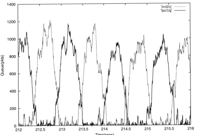
to understand ACK-Compression, as it affects the behavior and performance of a network, as later simulations will reveal.

ACK-compression results from an interaction between data and ACK packets when there

is two-way traffic and appears to require only two assumptions: "(1) ACK packets are

sig-nificantly smaller than data packets (2) the packets from different connections are clustered"

[32, page 8].

212 212.5 213 213.5 214

Time(secs)

214.5 215 215.5 216

Figure 2-2: Example of ACK-Compression

1400 1200 1000 800 600 400 CO a) 0i 'bnO/q' -'bnl/q' /

TCP is window-based and operates via an ACK-clocking mechanism. Because in normal circumstances, another packet is sent immediately upon the receipt of an ACK, the packets in an entire window become more or less clustered or clumped together. Thus, TCP exhibits the clustering in assumption (2). That ACK packets are much smaller than data packets, as assumed in (1), is generally true.

At the source, data packets are spaced by the transmission time of the data packet. At the receiver, an ACK is generated immediately upon the receipt of a data packet, so the spacing of packets is preserved and ACKs are separated according to the transmission time of a data packet. When ACKs encounter a congested router, however, they are queued. This causes them to lose their spacing (hence the term "compressed"). Upon leaving the queue, ACKs are separated by the transmission time of an ACK packet, which is smaller according to assumption (1). This disrupts the ACK-clocking, and is the key observation that triggers the ACK-compression phenomena.

One significant consequence of ACK-compression is that "... the number of packets that

can be in flight at any one time depends on how many compressed ACK's are in the pipe. Thus, there is no longer a well-defined capacity C that can reliably predict the occurrence of the congestion epochs." [32, page 17] The utilization suffers in both directions. A classic example of ACK-compression is depicted in Figure 2-2, which displays the queue size in both directions on a link.

2.4

Delay-bandwidth Product

The delay-bandwidth product or pipesize (P) of a link is a useful metric. Bandwidth (B) is the capacity, in packets per second, on a particular link interface. Delay (D) is the average round-trip time, in seconds, of TCP connections traversing the link. The product (D*B) indicates the total number of packets that can be in flight in both directions of the link at any instant.

In this thesis, the delay-bandwidth product is also used to set the buffer limit. It is a general rule of thumb to allocate enough buffer space to hold a pipesize worth of packets.

Chapter 3

AQM Background and Related Work

Congestion control in the Internet is a very broad topic. There are many flavors of differ-ent congestion control mechanisms. This chapter covers background on the Random Early Detection (RED) [16] algorithm and related congestion control algorithms.

[21] sets up a taxonomy that classifies different congestion control mechanisms for best-effort service according to four criteria: packet scheduling, buffer management, feedback, and end adjustments, all of which it deems necessary and sufficient. According to this taxonomy, RED is classified as both an indirect method of scheduling control and a queue management mechanism, with implicit feedback and a slow start end adjustment algorithm.

[31] presents another taxonomy for congestion control algorithms in packet switching

networks that is similar but based on control theory. Under this taxonomy, RED is classified as having closed loop control, (global) implicit feedback, and a slow start end adjustment algorithm. A number of recent papers take this control theoretic approach to analyzing RED

[3, 20, 18].

The studies in this thesis focus upon this class of algorithms 1 , and RED in particular.

To be precise, however, these classifications are really descriptions of the RED queue management strategy as coupled with the TCP end adjustment algorithm. It is interesting to observe how RED is designed with end system dynamics in mind. This was elaborated in Section 1.2.

Table 3.1: RED parameters

3.1

RED Algorithm

The Random Early Detection (RED) algorithm, has been the focus of much attention re-cently. This algorithm may be referred to as traditional or classic RED throughout this paper. RED emphasizes that it is able to avoid global synchronization and alleviate biases of bursty sources.

RED involves the setting of several parameters, which are preset in the router. Some of the parameter names used in this paper differ slightly from the original terminology, and is used for clarity. These are displayed in Table 3.1. The original terminology is shown in parentheses, if different.

A RED gateway detects incipient congestion by monitoring the average queue size.

This average queue size is calculated according to the following equation, an exponentially-weighted moving average (EWMA) of the instantaneous queue length:

aveq +- (1 - wq) * aveq

+

aveq represents the average queue value, and q is the size of the instantaneous queue. The

gain, wq, determines the time constant of this low pass filter.

As long as the average queue size remains below a "minimum threshold" (Bmin), all packets are let through and not dropped. When the average queue size grows such that it falls between Bmin and some "maximum threshold" (Bmax), packets are dropped at the gateway with a certain probability that is linearly correlated to the average queue size. This is illustrated in Figure 3-1, and the following equation.

RED parameter [function

Bmin (minth) minimum buffer threshold

Bmax (maxth) maximum buffer threshold

Pmax (max,) dropping probability at Bmax

buffer size hard queue limit

Pdrop 1.0 Pmax Pdrop 1.0 Pmax 0 B max Average Queue(pkts)

Figure 3-1: Original RED.

Bmin A B i2*B'max uup max

Average Queue (pkts)

Figure 3-2: Gentle RED.

aveq - Bmin

Pb +- Pmax *

Bmax - Bmirn

(3.2)

The effect of using the RED buffer management scheme is to keep average queue size low and overall throughput high, while reducing bias against bursty traffic [16].

Parameter Setting Some guidelines for setting RED parameters can be found in [13], and most RED tests and simulations in the recent literature follow these parameter guidelines.

Pmax (maxp): The suggested setting for Pmax is 0.1, which represents a maximum drop

rate of 10 percent. If the required steady-state drop rate exceeds this amount, we "assume that something is wrong in the engineering of the network, and that this is not the region that anyone wants to optimize." [13]

Bmax (maxth): It also suggests as a "rule of thumb" to set the maximum threshold Bmax

to three times the minimum threshold Bmin. This was changed from two times Bmin in the

1993 RED paper. [16]

Bmin (minth): Bmin must be big enough to allow a certain-sized burst to be absorbed.

0 Bmin ---

--I

---Gain, or wq: The gain, wq, determines the time constant of the filter, measured in packet

arrivals. The time constant is calculated by the formula: -1/ln(1 - wq) [16]. If the

instanta-neous queue changes from one value to another, this formula indicates the number of packet arrivals it takes for the average queue to move 63 percent of the way from the first value to the second. If the time constant is too small, transients will be captured in the averaged queue value. If the time constant is too long, the response of the average queue will be too

slow, and will become a poor reflector of the current queue level. Neither are desirable.

The appropriate setting of wq is dependent upon the link capacity according to the

following equation,

Wq = 1 - exp(-1/(T * C)) _(3.3)

where T is the time constant in seconds, and C is the link capacity in packets per second.

[15] says that RED achieves highest performance when the time constant is some multiple

of round-trips, rather than a fraction of a single round-trip time.

3.1.1

ECN

The performance of RED can be enhanced by setting a special bit in the Internet Protocol (IP) header, called the Explicit Congestion Notification (ECN) bit [11]. Upon the detection of incipient congestion, the RED gateway can turn on this ECN bit in the packet header rather than drop the packet. This packet is said to be "marked". When the marked packet arrives at its destination, the ECN bit is copied into the packet's acknowledgment that is sent back to the sender. Once the TCP sender receives the acknowledgement and detects that the ECN bit has been set, it can respond to the congestion notification as though it had just detected a dropped packet via duplicate acknowledgments. Thus, ECN allows congestion to be indicated to the end-host without dropping packets. Using ECN in this manner supposedly has the benefit of avoiding unnecessary packet drops and delays. This also allows TCP to retransmit and recover losses sooner, rather than rely on a costly coarse-grained timer. [11, 1, 14] (See Chapter 2 for further background on TCP.)

In order for this scheme to work, not only do the gateways need to be modified, but TCP senders need to be ECN-enabled, so that they know to check the bit. Most of the

simulations conducted in this paper turn on ECN. Note that wherever the term "dropping" is used within this paper, "marking" is also implied.

3.1.2

Gentle RED

The "gentle" version of RED was introduced to alleviate parameter sensitivity. It increases the packet drop rate gradually from Pmax to 1 as the average queue size grows from Bmax to 2 * Bmax [12]. Figures 3-1 and 3-2 show the difference between original RED and RED with the "gentle" addition.

Simulation tests show that even with less optimal settings of RED parameters Bmax and Pmax, gentle RED can still provide robust performance [10], and is with high confidence superior to the original RED. [33] claims that gentle RED performs well in heterogeneous environments involving FTP, Web, and UDP. Therefore, all RED or RED-related simulations conducted in this thesis use the "gentle" form of the algorithm.

3.2

Weaknesses of RED

Much experience has already revealed the difficulty in parameterizing RED queues to perform well under different levels of congestion and with different traffic mixes.

Many researchers have advocated not using RED [6, 24, 23] for various reasons. One of these reasons is that the tuning of RED parameters has been an inexact science, with some researchers resorting to trial-and-error as a means to find optimal settings. In addition, numerous RED variants have been proposed, some of which are discussed below. Many researchers have turned to mathematical analyses and have begun advocating a self-tuning, control-theoretic approach to RED [18, 7, 20]. The fact that these require no manual tuning relieves much of the burden in setting RED parameters accurately.

Some of the complexity in classic RED can be attributed to its parameter sensitivity. [15]

explains that RED is sensitive to the values of both wq and Pmax, and therefore these must

be carefully tuned in order to achieve good throughput and reasonable delays. The gentle version of the algorithm improves its robustness in this regard, in that increased traffic loads can be controlled by the more steeply increasing drop rate, even when the average queue

exceeds Bmax.

[15, Page 4] shows how, in classic RED, the link utilization and queue length can vary over

a range of Pmax and for various values of N. [13] acknowledges that the choice of parameters embodies "conscious design decisions" and that the optimal values are not known, and further that these optimal values "would depend on a wide range of factors including not only the link speed and propagation delay, but the traffic characteristics, level of statistical multiplexing, and such, for the traffic on that link. These decisions about average and maximum queue size are embodied not only in the choice of buffer size, but also in the choice for minth and

Wq."

If RED were ever to be widely deployed, it is highly important that RED be robust, and

that there be a systematic and straightforward way of setting parameters.

3.3

Related Work

It has become widely recognized that in order for RED to be robust, it needs to be adaptive. In order for a congestion control algorithm to be robust, it must be able to handle varying traffic loads. Furthermore, RED's static parameters (or, at least, parameters which must be reset manually) limit the range of traffic loads that it can handle.

Many new adaptive algorithms have been proposed in the past few years. There is yet to be a document that clearly classifies and benchmarks them all. This is not that document. However, we describe in some detail several of the relevant works to provide the reader with perspective. Some of these algorithms share common points of emphasis with one another and with the 2RegionRED algorithm we propose in Chapter 4. Their emphasis lies in one or more of the following:

* Adaptation to changing loads

" Decoupling of the congestion measure from the queue size " Use of the number of flows as a measure of congestion

3.3.1

Adaptive to Varying Traffic Loads: Variations on RED

The following algorithms are similar to RED in their mechanisms, but with parameters that adapt to changing environments. The common RED mechanisms are:

" Queue estimation using EWMA averaging " Probabilistic dropping probability

" The idea of keeping the queue within thresholds

In these algorithms, as in classic RED, queue length remains the indicator of the level of congestion or load.

Adaptive RED was originally proposed in [7], and adjusts Pmax in order to keep the

average queue length between Bmin and Bmax.

[15]

Adaptive RED, which automatically sets multiple parameters. Pmax is adapted in response to measured queue lengths to keep the averaged queue in a target range spanning a region half

way between Bmin and Bmax. Wq, the gain used in the queue estimator, is automatically

set based upon the link speed. Robustness of the algorithm is attributed to a very slow and gradual adaptation of Pmax using AIMD (Additive Increase Multiplicative Decrease). Simulations involving Adaptive RED congestion control can be found in Chapter 6.

Load Adaptive RED [3] takes another approach, leaving Pmax fixed, but dynamically

adjusting the Bmin and Bmax thresholds as the system load changes. The proposed mech-anism is to adjust the thresholds in such a way that the packet loss rate is kept close to a pre-specified target loss rate. This target loss rate is chosen as one that would prevent excessive timeouts among the TCP connections. In order to achieve the target loss rate, the

algorithm tries to maintain a constant packet dropping probability PA over time, according

to Equation 3.2. It notes loosely that as the number of flows vary causing the traffic load to increase or decrease, the average queue size aveq also increases or decreases respectively. In

order to maintain a constant Pb, as aveq changes, the thresholds can be adjusted accordingly,

3.3.2

Decoupling the Queue Length

The algorithms in the previous section use queue length as a congestion measure. A growing number of researchers have, however, become convinced that queue length alone is not a practical measure of congestion.

BLUE [8] emphasizes that decoupling the queue length from AQM schemes can provide

significant performance improvements. BLUE, evidently named because it is "a fundamen-tally different active queue management algorithm" from RED, uses buffer overflow and link idle events to adjust the packet marking/dropping probability for managing congestion. Upon sustained buffer overflow (which results in extensive packet loss), BLUE increments the marking probability by some factor. If on the other hand the link is idle, indicated by an empty queue, BLUE infers that its present dropping probability is too high, and so it decrements its marking probability.

REM or Random Exponential Marking [2] decouples what it calls the "congestion mea-sure" from "performance measures". A REM link computes some measure of congestion by measuring both the queue size ("buffer backlog") and the difference between the aggregate input rate and the link capacity. Common performance measures include loss rate, queue length, and delay. In REM, each link marks with a probability that is exponentially increas-ing in the congestion measure. REM stresses that this exponential relation is important when multi-bottleneck paths are considered, because of its effect on the end-to-end marking probability, or what it calls the "path congestion measure". The endhost is able to infer the path congestion measure from the fraction of marked packets it receives in a time inter-val. With knowledge of the path congestion measure, the source then adjusts its rate using some chosen marginal utility relation. Decoupling also allows flexibility in that the same exponential marking mechanisms can be used with different congestion measures.

3.3.3

Relation to the Number of Flows

Load-adaptive RED [3] points out that the number of flows affects congestion levels and that this is reflected in the size of the average queue. The Adaptive RED algorithm also

uses increasing queue size as a signal to increase its drop rate. However, the linear dropping probability curve that characterizes these variants of RED fails to capture the dynamics between the drop rate, number of flows, and the queue size.

Some algorithms therefore try to estimate the number of competing TCP flows N in a more direct manner. The drop rate is then adjusted accordingly. For these algorithms, the number of competing TCP connections is used as the measure of load or congestion.

FPQ Flow-Proportional Queuing [27] varies the router queue length proportionally to the

number of active connections. It estimates the number of active TCP connections using an algorithm that hashes connection identifiers of arriving packets into a small bit vector that is incrementally cleared. Once it has estimated N, FPQ determines what the target buffer size qt should be as a function of N using the following function. P, the pipesize, is the delay bandwidth product of the link.

targetQueue(N) qt +- max , 6N (3.4)

(2N - 1'

One consideration for the target queue is that for small N, the target buffer must be large enough so that full link utilization can be sustained. Notice for the target queue that as N

initially increases, qt decreases linearly according to P/(2N - 1). 6N is required at minimum

because six packet buffers are required per connection in order to avoid timeouts. Thus,

when N increases past a certain point, the queue length actually grows. 2

Once the target queue is computed, FPQ calculates the target loss rate. This is the dropping probability that hopefully will drive the queue length to the target buffer size.

targetLoss(qt, N) min 0.87 0.021 (3.5)

Notice that the loss rate is proportional to N2_{. The loss rate is chosen as that which would}

cause each of the N windows to be of size (P + qt)/N. This relies on the result that when a particular loss rate p is experienced by steady-state TCPs over a long period of time, the resulting average window size is inversely proportional to the square root of p [22].

2

W ~ P-1/2 _(3.6)

The loss rate is limited to a maximum of 0.021 or 2.1% loss rate because anything greater proved to have little impact on performance. By keeping the queue large enough so that each connection has a window of at least six packets on average, FPQ is able to avoid most timeouts, resulting in a more predictable queuing delay.

FPQ-RED FPQ can use the RED queue management scheme "to enforce its target queue

length and drop rate because of RED's ability to avoid oscillation" [26, Page 51]. When

N increases to the point where the target loss rate is limited to 2.1% and the target queue

grows proportionally to 6N, FPQ with RED can be thought of as a RED scheme that keeps Pmax fixed, but varies Bmax [27]. In this sense, FPQ and Load-Adaptive RED are similar in nature.

When FPQ is used with RED, [26, Page 47] has set Pmax to the targetLoss(qt, N),

Bmin to 5 packets, and Bmax to 2 * targetQueue(N). [26, Page 47] mentions a few possible

troublespots when using FPQ with RED. For instance, RED's linear queue length to drop rate function doesn't quite match that which FPQ needs. Also, the setting of the gain for the EWMA averaging of the queue length may require more damping. Nevertheless, some simulations of FPQ with RED are presented in Chapter 6 to illustrate the algorithm's main principles. In this thesis, we will refer to this variation on FPQ as FPQ-RED.

SRED Stabilized Random Early Drop [28] (SRED) is another algorithm that measures

load by estimating the number of active flows, though in a different manner. SRED uses a "zombie list" to estimate the number of flows. This is described in detail in [28]. Like FPQ, SRED derives some target buffer size based upon this knowledge of N and the average window

size, and then computes a drop rate, proportional to N2_{, whose aim is to drive the queue}

length to this target. The equations that SRED uses are more loosely derived but similar to those used in FPQ. Establishing the dropping probability only on the estimate of N can

lead to unpredictable buffer occupancy, because the p - N2 relation involves assumptions

things. Thus, the final drop rate imposed by SRED is also influenced by the actual queue size. SRED differs from FPQ in that SRED assumes a fixed buffer size.

3.3.4

Tradeoff between Throughput and Delay

RED-light is the congestion control algorithm proposed in the 1999 draft titled "RED in a Different Light" [20] .

RED-light notes that as the number of flows increases, the average queue size increases linearly while the drop rate increases in a quadratic relation. In an ideal world, one could

infer N from the average queue size and then administer a drop rate proportional to N2.

Because real world traffic is much more complex, RED-light focuses on finding an appropriate

operating point. 3

The authors of RED-light suggest setting Bmin, the target buffer size, to 0.3 * P where P

is the pipesize, or delay bandwidth product. They claim that this operating point represents:

1. a good balance between delay and utilization

2. a value that is able to absorb maximum bursts (bursts are also affected by the gain setting, which is described in detail in their paper) 4.

Between a fixed Bmin and Bmax, the drop rate increases in a quadratic manner with the queue size, to capture the relation between N, the size of the queue, and the drop rate. Note that there are some subtleties in the actual implementation of RED-light, which uses mechanisms that at least in appearance are radically different from RED. Also, a more deterministic method of dropping is used, rather than probabilistic.

3_{Caveat: Because [20] is a draft, some of these ideas are not completely articulated, and what is}

summa-rized here is the author's interpretation. 4

The paper proposes a new queue estimation scheme to track the persistent queue. What the appropriate

Chapter 4

2RegionRED, the Algorithm

In the previous chapter, we have seen that the task of setting up a RED gateway is made complex by the number of parameters involved and the need to understand how these pa-rameters are related to one another. We have also seen that it is difficult to parameterize RED to work effectively over varying levels of congestion. A workable RED would thus require maintenance in the setting and resetting of its parameters. The degree of human intervention that this involves is a clear invitation for human error to leak into the system, which is undesirable for the stability and clean operation of the Internet. For these reasons, it is of interest that a congestion control algorithm be:

" Simple. There should be an intuitively clear and systematic method of setting

param-eters (if any).

* Adaptive. The algorithm should be self-adjusting, requiring little or no manual tuning.

In this chapter we investigate a new adaptive RED algorithm, 2RegionRED. What distin-guishes this algorithm from the others is a set of principles that guide its design. We provide a clear and intuitive way of thinking about how these principles can be used to determine the drop rate that is appropriate at any time

These principles can be characterized by:

'This chapter summarizes and adapts ideas originally proposed in a 2000 draft by D. D. Clark titled "Slope-Controlled RED"

" Goals to maintain high utilization while keeping the persistent queue at a minimum

* A correlation between the number of flows, optimal buffer size, and drop rate

" Decoupling of the drop rate from the size of the queue

While these ideas are not new in themselves, we tie them together in a way that leads to a novel way of thinking about RED. The 2RegionRED algorithm is one product of this analysis.

Note that this section of the thesis attempts to work within the framework of the cur-rent Internet, leaving its protocols, structure, and state more or less intact. It leaves TCP unchanged, and focuses on the congestion control algorithm at the gateway.

4.1

Network Theory

4.1.1

An optimal RED signal: High link utilization, Low queuing

delay

One performance metric that most users care about is goodput, or the effective throughput that each user can attain. The congestion control algorithm operating at a gateway can have a significant effect upon user goodput. Its role in maximizing goodput is twofold, and involves minimizing the latency incurred at a router while maintaining high link utilization. Latency, or delay, is often used to quantify the quality of service delivered to a user, with better service characterized by less delay. There are four sources of delay that contribute to a user's perceived round-trip time. Propagation delay, the time it takes for a signal to propagate from one end of a link to another, is a result of the limitation imposed by the speed of light, and is therefore based upon the distance between source and destination, as well as physical factors such as the medium through which the bits are flowing. Serialization delay represents the time it takes to place a packet on the network. It is dependent upon the circuit speed; the higher the circuit speed, the less serialization delay. Packetization delay, the time it takes to collect enough bytes to fill a packet before it can be sent out, also contributes to the serialization delay. Finally, queuing delay is incurred when a packet has to wait in

some buffer along its path because there are other packets ahead of it in the queue waiting to be processed. Usually, propagation and queuing delay are the dominant contributors to latency. Whereas physical laws prevent us from minimizing propagation delay, congestion control algorithms can indirectly control the amount of queuing delay a user experiences by carefully controlling the drop rate.

In addition to minimizing queuing delay, maintaining high link utilization is also im-portant, because sustained periods of idleness on the link indicate that bandwidth is being wasted. This is wasted bandwidth that could have been used to increase connection through-puts. The congestion control algorithm should thus try to keep the link busy at all times.

These two goals of reducing the latency caused by queuing while keeping the link fully utilized translates into an optimal RED signal that keeps the buffer at a minimum, yet filled to the point such that it never goes to zero. We will revisit this important point in the next section.

4.1.2

The new RED signal: a more realistic RED signal

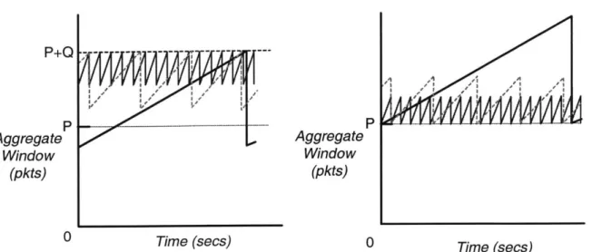
The optimal RED signal described above requires the algorithm to be omniscient, and is therefore not practical to implement. In this section we explain the new RED signal that is used in the design of 2RegionRED. This new RED signal tries to ensure full link utilization at the expense of some reasonable amount of queuing delay.

The role of buffers in routers is to absorb short time-frame bursts, as well as to buffer the packets that result from the congestion avoidance behavior of TCP, which involves the sawtooth in the window size as seen in Section 2.2.2.

As the various packet flows go through cycles of window increase and decrease, the aggregate occupancy of the buffer will go up and down, a phenomenon here called congestion

related buffer fluctuation, or just fluctuation (in contrast to fluctuation caused by transients

such as bursts). While in real networks the pattern of buffer fluctuation will be very complex, in a simplified analysis there is a well defined fluctuation behavior that will result depending on how congestion is signaled.

Figure 4-1 depicts the size of the congestion window for three individual TCP flows whose paths share a common outgoing link interface, and whose connection properties (RTT,

bottleneck, etc.) are identical. Their aggregate window, which is simply a sum of the individual windows per unit time, is also depicted. The aggregate represents the number

of packets that arrive at this link interface each round-trip time.

Q

depth, or allocated buffer size. P represents the pipe size, which is the equivalent of the link capacity, or delay-bandwidth product for this link. If the incoming traffic exceeds the link capacity P, the excess is buffered and a queue begins to form. Thus, the shape of the queue roughly matches the shape of the aggregate window above P.

Aggregate

Q.

0

Time (secs)

0

_Time(secs)

Figure 4-1: Windows of three TCP flows in congestion avoidance

Aggregate

P

Window

(pkts)

0

Time (secs)

Time(secs)

Figure 4-2: Desired dropping behavior for new RED signal

P+Q.

Window

(pkts)