HAL Id: hal-02593068
https://hal.inrae.fr/hal-02593068
Submitted on 12 Oct 2020
HAL is a multi-disciplinary open access
archive for the deposit and dissemination of
sci-entific research documents, whether they are
pub-lished or not. The documents may come from
teaching and research institutions in France or
abroad, or from public or private research centers.
L’archive ouverte pluridisciplinaire HAL, est
destinée au dépôt et à la diffusion de documents
scientifiques de niveau recherche, publiés ou non,
émanant des établissements d’enseignement et de
recherche français ou étrangers, des laboratoires
publics ou privés.
CBGP: Classification Based on Gradual Patterns
Yeow Wei Choong, Lisa Di Jorio, Anne Laurent, Dominique Laurent,
Maguelonne Teisseire
To cite this version:
Yeow Wei Choong, Lisa Di Jorio, Anne Laurent, Dominique Laurent, Maguelonne Teisseire. CBGP:
Classification Based on Gradual Patterns. International Conference of Soft Computing and
Pat-tern Recognition (SoCPaR), Dec 2009, Malacca, Malaysia. pp.7-12, �10.1109/SoCPaR.2009.15�.
�hal-02593068�
CBGP: Classification Based on Gradual Patterns
Yeow Wei Choong HELP University College
Dept. of IT Kuala Lumpur - Malaysia
Lisa Di Jorio, Anne Laurent LIRMM Univ Montpellier 2 - CNRS Montpellier - France {dijorio,laurent}@lirmm.fr Dominique Laurent ETIS
Univ Cergy Pontoise - CNRS Cergy Pontoise - France
[email protected] Maguelonne Teisseire CEMAGREF UMR Tetis Montpellier - France [email protected]
Abstract—In this paper, we address the issue of mining gradual classification rules. In general, gradual patterns refer to regularities such as “The older a person, the higher his salary”. Such patterns are extensively and successfully used in command-based systems, especially in fuzzy command appli-cations. However, in such applications, gradual patterns are supposed to be known and/or provided by an expert, which is not always realistic in practice.
In this work, we aim at mining from a given training dataset such gradual patterns for the generation of gradual classification rules. Gradual classification rules thus refer to rules where the antecedent is a gradual pattern and the conclusion is a class value.
Keywords-data mining; classification; gradual rules
I. INTRODUCTION
Classification is a key problem in many real world applications that aim at determining the class of objects knowing their values over a given set of attributes. For instance, considering gene analysis applications, determining whether a tumor is malignant or not based on observed gene expressions is a key issue.
In this framework, many methods have been defined, e.g., decision trees, naive bayes, neural networks, SVMs, (see [9], [17]), some of these methods being more explica-tive/understandable for the user than other ones. In partic-ular, decision tree-based approaches, such as C4.5 ([18]), provide the user with a set of rules (so-called classification rules) that explicitly show why an example has been labeled with a particular class.
In this paper, we address the problem of computing classification rules when traditional approaches fail, because considering attribute values as such is not appropriate. In such a case, we look for trends shown by sets of values over the same attribute, such as the higher/lower the value of attributeA, the higher/lower the value of attribute B.
For example, in gene analysis, it could be the case that the values of gene expressions do not allow for any prediction regarding the malignancy of a tumor, whereas sets of such values contain trends like the more gene G1 is expressed, the less geneG2 is expressed, when the tumor being considered is malignant. Therefore, this type of gradual rule can be used to determine whether a given new tumor is malingnant.
For this purpose, we consider gradual patterns to describe trends in a given training dataset, thus leading to a novel and appealing rule-based classification method, extending existing methods such as CBA (Classification Based on Association rules) [14] or SPaC (Sequential Patterns for Classification) [11].
The paper is organized as follows: Section II introduces a running example considered throughout the paper to il-lustrate our approach. In Section III, we review previous work on gradual rules and rule-based classification methods. In Section IV, we introduce the basic definitions related to gradual frequent patterns and gradual classification rules. In Section V, we report on the experiments we have conducted to assess our method, and Section VI concludes the paper and provides further research directions.
II. RUNNINGEXAMPLE
To illustrate our approach, we consider the (toy) example described in Table I, referring to fruit quality measurement as a mean to determine their provenance.
In this case, we assume that fruits, with properties size (S), weight (W ) and sugar rate (SR), are delivered in box containers that have to be dispatched according to their provenance. Assuming that this provenance is ignored, we try and predict it, knowing that two provenances (i.e., two classes) are possible, namely N orth and South.
As argued next, it turns that in Table I, the size-, weight-and sugar rate values of fruits, considered one by one, do not allow for the prediction of the provenance, meaning that traditional classification approaches fail to predict fruit provenance based on their size, weight and sugar rate.
On the other hand, it will be seen shortly that, considering gradual patterns (i.e., tendencies of the size-, weight- and sugar rate values) allows to characterize the provenance.
As mentioned above, traditional classification methods do not apply in this example as no generality can be extracted tuple by tuple. Indeed, under Weka environment:
• Running C4.5 gives:
J48 pruned tree ——————
Id Size Weight Sugar Rate Provenance t1 6 6 5.3 N orth t2 10 12 5.1 N orth t3 14 4 4.9 N orth t4 23 10 4.9 N orth t5 6 8 5.0 South t6 14 9 4.9 South t7 18 9 5.2 South t8 23 10 5.3 South t9 28 13 5.5 South Table I
TRAININGSET: FRUITPROVENANCES
Id Size Weight Sugar Rate n1 4 7 5.3 n2 18 14 5.0 n3 22 6 4.9 n4 16 9 6.1 Table II TESTSET: NEWFRUITS
This means that the classifier predicts all fruit prove-nances be equal to South as the corresponding class contains most examples. The accuracy of this model (evaluated using cross validation) is very low, that is 11.11% (4 exceptions over 9 examples as reported in the brackets), meaning that this model fails to predict the provenance in 88.89% of the cases.
• Similarly, running a Naive Bayes method, a multilayer perceptron method and the KNN method gives a pre-diction accuracy of, respectively, 33%, 22.22% and 33.3333%.
Thus, clearly, whatever the method, attribute values as such can not determine fruit provenance, due to the fact that all fruits have almost the same size, weight and sugar rate (implying that standard classification methods cannot avoid over-fitting).
However, we argue that the way these attributes co-variate can help determining fruit provenance. Indeed, it can be seen from Table I that in general:
• For fruits from North, the higher the size, the lower
the sugar rate(referring to the first four tuples); but no correlation involving the weight can be found.
• For fruits from South, the higher the size, the higher the weight, the higher the sugar rate (referring to the last five rows except tuple t2).
In our apporach, we formalize these tendencies through the following two gradual classification rules:
• {(S, ≥), (SR, ≤)} ⇒ N orth, and • {(S, ≥), (W, ≥), (SR, ≥)} ⇒ South
Consider now a new set of fruits, known to have the same provenance, but which has to be determined. The measurements of these fruits, reported in Table II, show that the pattern the higher the size, the lower the sugar rate holds.
As this gradual pattern holds in Table I for northern fruits and not for southern fruits, the fruits described in Table II are considered as northern fruits, which can not be found using any traditional classification approach, as shown above.
III. RELATEDWORK A. Gradual Rules
Gradual patterns and gradual rules have been studied for many years in the framework of control, command and recommendation. More recently, data mining algorithms have been studied in order to automatically mine such patterns [3], [4], [5], [7], [10].
The approach in [10] uses statistical analysis and linear regression in order to extract gradual rules. In [3], the authors formalize four kinds of gradual rules in the form The more/less X is in A, then the more/less Y is in B, and propose an Apriori-based algorithm to extract such rules. However, frequency is computed from pairs of objects, increasing the complexity of the algorithm. Despite a good theoretical study, the algorithm is limited to the extraction of gradual rules of length 3.
The approach in [7] is the first attempt to formalize grad-ual sequential patterns. This extension of itemsets allows for the combination of gradual temporality (“the more quickly”) and gradual list of itemsets. The extraction is done by the algorithm GRaSP, based on generalized sequential patterns [16] to extract gradual temporal correlations.
In [4] and [5], two methods to mine gradual patterns are proposed. The difference between these approaches lies in the computation of the support: whereas, in [4], a heuristic is used and an approximate support value is computed, in [5], the correct support value is computed. It is important to note in this respect that, in the current paper, the method of [5] is used for the computation of frequent gradual patterns. We refer to Section IV for the corresponding formal definitions. B. Classification Based on Rules
Classification has been extensively studied [17]. In this paper, we focus on classification based on rules as this is the method we aim at extending.
In [14] the authors propose a text categorization method based on association rules, called CBA. The method consists of two steps: (i) rule generation (CBA-RG), based on the well-known Apriori algorithm, and (ii) building the classifier (CBA-CB), based on generated rules.
In the first step, each assignment of a text to a category is represented by a pair ρ = hcondset, Cii, called a ruleitem,
and where condset is a set of items and Ci is a class
label. Each ruleitem ρ should be thought of as a rule condset → Ci, whose support and confidence are defined
supp(ρ) = #texts from Cimatching condset
#texts in D
conf (ρ) = #texts in Cimatching condset
#texts in D matching condset
Ruleitems whose support is above a given threshold are said to be frequent, and the set of class association rules (CARs) consists of all frequent ruleitems whose confidence is greater than a minimum confidence threshold. Once all CARs are generated, they are totally ordered according to the following precedence relation: If ri and rj are two CARs, ri ≺ rj
(precedes) if:
• either conf (ri) > conf (rj)
• or conf (ri) = conf (rj) and supp(ri) > supp(rj) • or conf (ri) = conf (rj) and supp(ri) = supp(rj) and
ri has been generated before rj.
Let R be the set of CARs and D the training data. The basic idea of the algorithm is to choose a set of high precedence rules in R to cover D. The categorizer is represented by an ordered list of rules ri ∈ R, leading to pairs such as
h(r1, r2, ..., rk), Cii, where Ci is a target category.
Each rule is then tested on D. If a rule does not improve the accuracy of the classifier, this rule and the following ones are discarded from the list.
Once the categorizer has been built, each ordered rule ri ∈ R is tested on every new text to classify. As soon as
the condset part of a rule is supported by the text, the text is then assigned to the target class of the rule.
Many other research has been done using association rules for classification. In [12], the authors replace the confidence by the intensity of implication. In [13], the authors integrate the CBA method with other methods such as decision trees, Naive Bayes, RIPPER, etc. to increase the classification score. In [2], the authors investigate a method for association rule classification called L3. Contrary to CBA-CB which
takes only one rule into account, the authors propose to determine the category of a text by considering several rules, using a majority voting.
In [1], association rules are used for partial classification. Partial classification means that the classifier does not cover all cases. In particular, this work is interesting when dealing with missing values.
CAEP [6], LB, ADT [19], CMAR [15] are other existing classification systems using association rules. LB and CAEP are based on rule aggregation rather than rule selection. ARC-CB [20] proposes a solution for multi-classification (i.e., a text is associated to one or more classes).
To end the section, we emphasize that none of these clas-sification approaches have considered using gradual patterns, as we do in this paper.
IV. CBGP: CLASSIFICATIONBASED ONGRADUAL PATTERNS
In this section, we detail our proposal for Classification Based on Gradual Patterns. We recall that our approach
is composed of two parts: first we compute the gradual patterns representing each class value (thus constructing the gradual pattern-based classifier), and then we define how to determine the class values of new examples. We recall that the notions of gradual itemsets and their support are borrowed from [5]; these definitions are stated next. A. Basic Definitions
In this work, we assume that we are given a database DB that consists of a single table whose tuples are defined on the attribute set I. In this context, gradual patterns are defined to be subsets of I whose elements are associated with an ordering, meant to take into account increasing or decreasing variations.
In the definitions given below, using standard notation from the relational database model, for each tuple t in DB and each attribute I in I, t[I] denotes the value of t over attribute I.
Definition 1: (Gradual Itemset) Given a table DB over the attribute set I, a gradual item is a pair (I, θ) where I is an attribute in I and θ a comparison operator in {≥, ≤}.
A gradual itemset g = {(I1, θ1), ..., (Ik, θk)} is a set of
gradual items of cardinality greater than or equal to 2. We point out that gradual itemsets are assumed to be sets of cardinality greater than or equal to 2, because sorting tuples according to one attribute is always possible, which is not the case when considering more than one attribute.
The support of a gradual itemset in a database DB is defined as follows.
Definition 2: (Support of a Gradual Itemset) Let DB be a database and g = {(I1, θ1), ..., (Ik, θk)} a gradual itemset.
The cardinality of g in DB, denoted by λ(g, DB), is the length of the longest list l = ht1, . . . , tni of tuples in DB
such that, for every p = 1, . . . , n−1 and every j = 1, . . . , k, the comparison tp[Ij] θjtp+1[Ij] holds.
The support of g in DB, denoted by supp(g, DB), is the ratio of λ(g, DB) over the cardinality of DB, which we denote by |DB|. That is, supp(q, DB) = λ(g,DB)|DB| .
In order to compute λ(g, DB), [5] proposes to consider the graph where nodes are the tuples from DB and where there exists a vertex between two nodes if the corresponding tuples can be ordered according to g.
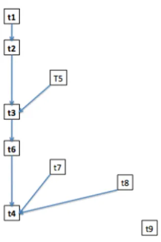
Example 1: Referring back to our running example, since we aim at building rules to determine fruit provenance, the table DB to be considered for the definition of gradual itemsets is the projection of Table I over the attributes S, W and SR. In other words, we consider that I = {S, W, SR}. Figure 1 shows the ordering of the tuples of DB, accord-ing to the gradual itemset g = {(S, ≥), (SR, ≤)}, whose intuitive meaning is the higher the size, the lower the sugar rate. As in this graph, the length of the longest totally ordered list of tuples is 5, and as DB contains 9 tuples, we have supp(g, DB) =59.
Figure 1. Graph of g = {(S, ≥), (SR, ≤)} as computed on Table I
Consider now the tuples in DB whose Provenance value is N orth, i.e., the first four tuples in DB. Denoting this set by DB(N orth), we have supp(g, DB(N orth)) = 1. B. Building the GP-Based Classifier
Considering a training database, i.e., a set of tuples representing examples whose class is known, we aim at building a classification model based on frequent gradual itemsets, as done in CBA-like methods.
The two step processing works as follows: During the first step, frequent gradual itemsets are computed for each class. Then, during the second step, for every class, the correspond-ing gradual rules are defined based on the frequent gradual itemsets previously computed. The quality of these gradual rules is assessed, based on the notion of discriminance of a given rule that measures to which extent a gradual rule is representative of the class it has been extracted from.
More formally, let C be a set of class values, and I be a set of attributes, we aim at building a set of gradual classification rules in the form g ⇒ c where g is a gradual itemset and c ∈ C.
The training database, denoted by DBT, is defined over
the attribute set I ∪ {C}. Intuitively, every tuple in DBT is
characterized by its values over attributes in I and its class value, stored as an attribute value.
Table I shows an example of such a training database, in which the set C of class values is {N orth, South}, seen as the domain of the attribute showing the provenance.
The table DBT is partitioned according to the values in
C, and for every c in C, we denote by DBT(c) the set of all
restrictions over I of all tuples in DBT where the class value
is c. That is, DBT(c) = {t[I] | t ∈ DBT and t[C] = c}.
Given an itemset g over I, the support of g in class c is the support of g in DBT(c), that is, according to Definition 2,
supp(g, DBT(c)), which we denote by supp(g, c) for the
sake of simplification.
Given a minimum support threshold minsup, for ev-ery class value in C, all gradual itemsets g such that supp(g, c) ≥ minsup are computed using the method of [5]. These gradual patterns are then considered in order to define whether they are discriminant for the class. The discriminance measureis defined as follows.
Definition 3: (Discriminance of a Gradual Itemset) Let g be a gradual itemset and c be a class value in C. Denoting by Γ(g) the set of all class values γ such that supp(g, γ) ≥ minsup, the discriminance of g regarding c is defined as:
disc(g, c) = Psupp(g, c)
γ∈Γ(g)
supp(g, γ).
Given a support threshold minsup and a discriminance threshold mindisc, the problem of building a set of gradual classification rules amounts to computing, for every class value c in C, the set of all rules of the form g ⇒ c such that supp(g, c) ≥ minsup and disc(g, c) ≥ mindisc.
In what follows, we denote by Gc the set of all gradual
itemsets g such that supp(g, c) ≥ minsup and disc(g, c) ≥ mindisc.
Example 2: Referring back to our running example, con-sider minsup = 0.75 and mindisc = 0.25.
It can be seen that for the class value N orth, g = {(S, ≥), (SR, ≤)} is the only gradual itemset such that supp(g, N orth) ≥ minsup. Therefore, the only rule to be considered in this case is {(S, ≥), (SR, ≤)} ⇒ N orth, and by Definition 3, disc(g, N orth) = 1. Thus GN orth= {g}.
For the class value South, the frequent gradual itemsets are g1 = {(S, ≥), (SR, ≥)}, g2 = {(S, ≥), (W, ≥)}, g3 =
{(W, ≥), (SR, ≥)} and g4 = {(S, ≥), (W, ≥), (SR, ≥)},
with respective supports in DBT(South) 45, 1, 4
5 and
4 5.
Thus, Γ(South) = 175, and so, disc(g2, South) = 175 ≥
0.25 and for i = 1, 3 or 4, disc(gi, South) = 174 < 0.25.
Therefore, GSouth = {g2}.
Gradual classification rules are used for the classification of new examples, as shown below.
C. Classification of New Examples
Considering the classification rules constructed in the pre-vious step, we address the issue of labelling new examples where the class values are unknown. We consider in this respect that we are provided with:
1) either a set of tuples known to be of the same class, 2) or a single tuple.
Notice that, in the second case above, a set of tuples not known to be of the same class can be considered. In this case, the tuples are processed one by one.
1) Set of Tuples of the Same Class: Let DBN ew be a
set of tuples, known to be of the same class that has to be determined. In this case, we first extract all frequent grad-ual itemsets from DBN ew, considering the same minsup
threshold as above. Denoting this set by GN ew, in order to
compute which class is the most appropriate, we compare GN ew to every Gc. The class cN ewissued by our method is
such that: cN ew= argmaxc∈C X g∈GN ew (disc(g, c)) where disc(g, c) = 0 if g 6∈ Gc
Example 3: Let us consider the set of fruits as described in Table II, where the common provenance is ignored. It is easy to see that GN ew contains the only gradual itemset
g = {(S, ≥), (SR, ≤)} with support 0.75. Since g ∈ GN orth
and g 6∈ GSouth, we obtain cN ew = N orth, meaning that
the fruits are considered from the North.
2) Single Tuple: We now assume that we are provided with a single tuple t defined over I. Computing the class of t is achieved as follows: for every class value c and every g in Gc, we compute to which extent t complies with g, as
described in Algorithm 1. The criterion introduced to this end, called relevance of c, is denoted by rel(c).
Data: t a tuple defined over I ; Result: cN ew ; foreach c ∈ C do rel(c) ← 0 ; foreach g ∈ Gcdo s ← supp(g, DBT(c) ∪ {t}) ; if s ≥ supp(g, DBT(c)) then
rel(c) ← rel(c) + disc(g, c) end
end end
cN ew← argmaxc∈C(rel(c)) ;
Algorithm 1: Classifying a new tuple
It should be noticed that computing supp(g, DBT(c) ∪
{t}) can be performed incrementally provided that the ordering graphs are stored when constructing the frequent gradual itemsets of Gc. In this case, the computation simply
amounts to inserting the new tuple within the graph. It is easy to see that, if the insertion results in a longer maximal ordered list then s ≥ supp(g, DBT(c)), else the test fails.
Example 4: Referring back to our running example, for the thresholds minsup = 0.75 and mindisc = 0.25, let n = (12, 14, 5.0) (over attributes S, W and SR) be a new tuple to be classified.
As seen in Example 2, for the class value N orth,
GN orth = {g} where g = {(S, ≥), (SR, ≤)} and
disc(g, N orth) = 1. Since supp(g, DBT(N orth) ∪ {n}) =
1 (by inserting n between t2 and t3), we obtain that
rel(N orth) = 1.
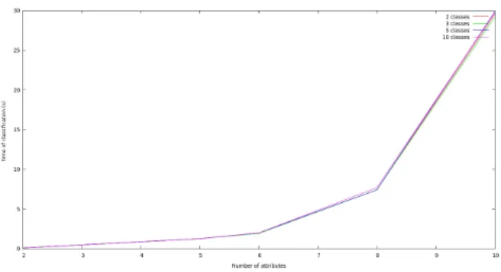
Figure 2. Runtime for Classifying New Tuples With Respect to the Number of Attributes
For the class value South, it has been seen in Exam-ple 2 that GSouth = {g2} where g2 = {(S, ≥), (W, ≥)},
supp(g2, South) = 1 and disc(g2, South) = 175.
Moreover, supp(g2, DBT(South) ∪ {n}) = 56
(since n cannot be inserted in DBT(South) so
as to preserve the ordering according to g2). Thus,
supp(g2, DBT(South) ∪ {n}) < supp(g2, DBT(South)),
showing that rel(South) = 0. Hence, cN ew= N orth.
V. EXPERIMENTS
In this section, we report on preliminar experiments conducted to assess our approach on synthetic data sets. We show that the runtime for classification new examples is not prohibitive, assuming that gradual rules have been mined.
To this end, the following criteria have been considered, in the case where a set of 500 new examples known to be of the same class value is considered: the size of the database, the number of class values, and the number of attributes.
Figure 2 reports on the runtime for classifying a set of 500 new tuples regarding the number of attributes. We notice that the number of underlying class values in C has a very low impact on runtime, showing that the runtime is constant whatever the number of class values.
On the other hand, it can be seen that, for up to 6 attributes, runtime is far below 5 seconds, and that, for 6 up to 8 attributes, runtime does not exeed 10 seconds. It should be noticed in this respect that, as reported in [3], most existing approaches for mining gradual rules encounter difficulties when handling more than 6 attributes.
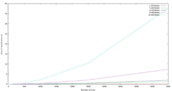
Figure 3 reports on the runtime regarding the size of the training database DBT, when classifying 500 new examples.
In particular, this figure shows that for less than 10 attributes in I, the increase of runtime is not significant (since less than 10 seconds for up to 5000 tuples in DBT), whereas for 10
attributes (and more) this increase is more important. Clearly, more experiments are needed in order to better assess our approach. In particular, we plan to consider real data sets collected from satellite pictures for the classifica-tion of land areas, according to the type of farming. Indeed,
Figure 3. Runtime for Classifying New Tuples With Respect to the Size of the Database
it has been identified that standard classification methods do not perform satisfactorily in this context, and it is expected that gradual classification rules can give relevant results.
VI. CONCLUSION
In this paper, we have proposed a novel classification method based on gradual rules. In this context, we have provided an approach for computing gradual rules and for assigning a class value to new examples. The experiments reported in this paper show that our approach is tractable.
Further work include conducting more experiments to better assess the performance and the relevance of our approach. We also intend to investigate other measures to determine to what extent a new tuple t complies with a gradual pattern g. The heuristic presented in [4] will be investigated in this respect, as well as the computation of the number of attributes that prevent a tuple t to be inserted according to the ordering specified by a given gradual itemset. We also intend to study how to efficiently maintain the discriminence updated when new examples are inserted in the training database.
ACKNOWLEDGMENT
The authors acknowledge Fabien Millet, a Master Student at the Polytech’Montpellier Engineering School, University of Montpellier 2 for his work in implementing and testing the methods and algorithms presented in this paper.
REFERENCES
[1] K. Ali, S. Manganaris and R. Srikant. Partial Classification Using Association Rules. In Knowledge Discovery and Data Mining, 1997.
[2] E. Baralis and P. Garza. Majority Classification by Means of Association Rules. In Proc. European Conf. on Principles and Practice of Knowledge Discovery in Databases(PKDD), 2003. [3] F. Berzal, J.C. Cubero, D. Sanchez, M.A. Vila and J.M. Serrano. An Alternative Approach to Discover Gradual De-pendencies. In Int. Journal of Uncertainty, Fuzziness and Knowledge-Based Systems(IJUFKS), 15(5), 2007.
[4] L.D. Jorio, A. Laurent and M. Teisseire. Fast Extraction of Gradual Association Rules: A heuristic based method. In Proc. Int. Conf. on Soft Computing as Transdisciplinary Science and Technology(CSTST), 2008.
[5] L.D. Jorio, A. Laurent and M. Teisseire. Mining Frequent Gradual Itemsets from Large Databases. In Proc. Intelligent Data Analysis Conf.(IDA), LNCS, Springer-Verlag, 2009. [6] G. Dong, X. Zhang, L. Wong and J. Li. CAEP: Classification
by Aggregating emerging patterns. In Proc. Int. Conf. on Dis-covery Science(DS’99), LNAI 1721, Springer-Verlag, 1999. [7] C. Fiot, F. Masseglia, A. Laurent and M. Teisseire. Gradual
Trends in Fuzzy Sequential Patterns. In Proc. Int. Conf. on Information Processing and Management of Uncertainty in Knowledge-based Systems(IPMU), 2008.
[8] S. Galichet, D. Dubois and H. Prade. Categorizing Classes of Signals by Means of Fuzzy Gradual Rules. In Proc. Int. Joint Conf. on Artificial Intelligence(IJCAI), 2003.
[9] J. Han and M. Kamber, Data Mining Concepts and Techniques, Morgan Kaufmann Pub., 2000.
[10] E. H¨ullermeier. Association Rules for Expressing Gradual Dependencies. In Proc. European Conf. on Principles of Data Mining and Knowledge Discovery(PKDD), 2002.
[11] S. Jaillet, A. Laurent, M. Teisseire. Sequential Patterns for Text Categorization. in Int. Journal of Intelligent Data Analy-sis, 10(3), 2006.
[12] D. Janssens, G. Wets, T. Brijs, K. Vanhoof and G. Chen. Adapting the CBA-Algorithm by Means of Intensity of Im-plication. In Proc. Int. Conf. on Fuzzy Information Processing Theories and Applications, 2003.
[13] B. Liu, Y. Ma and C.K. Wong. Classification Using Associ-ation Rules: Weaknesses and Enhancements. In Data mining for scientific application, 2001.
[14] B. Liu, W. Hsu and Y. Ma. Integrating Classification and Association Rule Mining. In Knowledge Discovery and Data Mining, 1998.
[15] W. Li, J. Han and J. Pei. CMAR: Accurate and Efficient Classification Based on Multiple Class-Association Rules. In Proc. Int. Conf. on Data Mining (ICDM), 2001.
[16] F. Masseglia, P. Poncelet and M. Teisseire. Pre-processing Time Constraints for Efficiently Mining Generalized Sequential Patterns. In Proc. Int. Symposium on Temporal Representation and Reasoning(TIME ’04), 2004.
[17] Tom Mitchell. Machine Learning. McGraw Hill, 1997. [18] J. Quinlan. C4.5 - Programs for Machine Learning. Morgan
Kaufman, 1993.
[19] K. Wang, S. Zhou and Y. He. Growing Decision Trees on Support-Less Association Rules. In Knowledge Discovery and Data Mining, 2000.
[20] M.L. Antonie and O.R. Zaiane. Text Document Categoriza-tion by Term AssociaCategoriza-tion. In Proc. Int. Conf. on Data Mining (ICDM), 2002.
View publication stats View publication stats