Advanced Process Data Analytics
by
Weike Sun
B.S., Tsinghua University (2015)
Submitted to the Department of Chemical Engineering
in partial fulfillment of the requirements for the degree of
Doctor of Philosophy
at the
MASSACHUSETTS INSTITUTE OF TECHNOLOGY
May 2020
© Massachusetts Institute of Technology 2020. All rights reserved.
Author . . . .
Department of Chemical Engineering
May 1, 2020
Certified by. . . .
Richard D. Braatz
Edwin R. Gilliland Professor in Chemical Engineering
Thesis Supervisor
Accepted by . . . .
Patrick S. Doyle
Chairman, Department Committee on Graduate Theses
Advanced Process Data Analytics
by
Weike Sun
Submitted to the Department of Chemical Engineering on May 1, 2020, in partial fulfillment of the
requirements for the degree of Doctor of Philosophy
Abstract
Process data analytics is the application of statistics and related mathematical tools to data in order to understand, develop, and improve manufacturing processes. There have been growing opportunities in process data analytics because of advances in ma-chine learning and technologies for data collection and storage. However, challenges are encountered because of the complexities of manufacturing processes, which of-ten require advanced analytical methods. In this thesis, two areas of application are considered. One is the construction of predictive models that are useful for process design, optimization, and control. The other area of application is process monitoring to improve process efficiency and safety.
In the first area of study, a robust and automated approach for method selection and model construction is developed for predictive modeling. Two common challenges when building data-driven process models are addressed: the high diversity in data quality and how to select from a wide variety of methods. The proposed approach combines best practices with data interrogation to facilitate consistent application and continuous improvement of tools and decision making.
The second area of study focuses on process monitoring for complex manufacturing systems, which includes fault detection, identification, and classification. Four sets of algorithms are developed to address limitations of traditional monitoring methods. The first set provides the optimal strategy for Gaussian linear processes, including deep understanding of the process monitoring structure and optimal fault detection based on a probabilistic formulation. The second set aims at building a self-learning fault detection system for changing normal operating conditions. The third set is developed based on information-theoretic learning to address limitations of second-order statistical learning for both fault detection and classification. The fourth set tackles the problem of nonlinear and dynamic process monitoring.
The proposed methodologies and algorithms are tested on several case studies where the value of advanced process data analytics is demonstrated.
Thesis Supervisor: Richard D. Braatz
Acknowledgments
It has been an extraordinary privilege to have been given the opportunity to pur-sue my doctoral degree at MIT and work on research that I find both interesting and consequential. I have had the opportunity to work with incredible mentors and collaborators without whom my Ph.D. would have been a very different experience.
I would like to first thank my advisor, Richard D. Braatz, for giving me the re-search opportunity and being an exceptional mentor throughout the years. His gen-erosity with this time, energy, and intellect in advising me was boundless. He gave me critical feedback on my research and asked questions that I would have never thought to consider. He also provided me with candid advice with my career development and the list of things that I learned is too long to articulate here. Besides, I would like to express my gratitude to my thesis committee members George Stephanopoulos and James Swan for valuable conversations and contributions to my research. I would also like to thank ExxonMobil and U.S. Food and Drug Administration for funding. I am appreciative of my fellow students and all of my lab mates for the help and company. In particular, I would like to thank Zhe Yuan, Zhenshu Wang, and Ruihao Zhu for helping me with my coursework as well as being great friends outside of the class. Kristen Severson and Wit Chaiwatanodom for providing help with my research. Matthias VA for being an excellent collaborator during my teaching experience. Ana Nikolakopoulou and Amos Lu for the help with the cluster. And all of my teammates at practice school for the company, conversation, and hard work.
I was fortunate to have internship experiences in several companies across different industries. I am indebted to the support, guidance, and encouragement given by my colleagues and mentors during my time at Takeda, General Mills, and ExxonMobil. I am particularly appreciative of Peng Xu and Antonio Paiva at ExxonMobil for helping me sharpen both my technical and communication skills. Also, Arash Fathi for the encouragement and making my day-to-day work enjoyable.
Finally, I would like to thank my family and friends for their tremendous amount of support over the past five years.
Contents
Introduction
35
1 Introduction 37
1.1 Thesis goals . . . 37
1.2 Thesis organization . . . 38
I
Advanced Predictive Modeling
43
2 Introduction to Predictive Modeling 45 2.1 Linear Regression with Penalty . . . 472.2 Partial Least Squares . . . 49
2.3 Support Vector Regression . . . 51
2.4 Random Forest Regression . . . 52
2.5 Linear state-space model . . . 53
2.6 Summary of the Contributions in Part I . . . 53
3 ALVEN: Algebraic Learning Via Elastic Net for Static and Dy-namic Nonlinear Model Prediction 55 3.1 Introduction . . . 55 3.2 Background . . . 57 3.3 ALVEN . . . 58 3.4 DALVEN . . . 61 3.5 Case Studies . . . 64 3.5.1 3D printer . . . 64
3.5.2 CSTR . . . 67
3.6 Conclusion . . . 69
4 Smart Process Analytics for Predictive Modeling 73 4.1 Introduction . . . 73
4.2 A Framework for Predictive Modeling . . . 74
4.2.1 A systematic approach for robust and automated predictive modeling . . . 74
4.2.2 Why not try every possible model and pick the “best” one . . 76
4.3 Data Interrogation . . . 81
4.3.1 Nonlinearity . . . 81
4.3.2 Multicollineraity . . . 83
4.3.3 Dynamics . . . 84
4.3.4 Heteroscedasticity . . . 85
4.4 Method Selection: Data Analytics Triangle . . . 86
4.4.1 Methods for multicollinearity . . . 86
4.4.2 Methods for Nonlinear Model Construction . . . 94
4.4.3 Methods for dynamics . . . 95
4.5 Hyperparameter Selection for Automated Model Construction . . . . 103
4.5.1 Simple held-out validation set . . . 104
4.5.2 𝐾-fold cross-validation . . . 104
4.5.3 Repeated 𝑘-fold and Monte Carlo (MC) based cross-validation 105 4.5.4 Grouped cross-validation . . . 105
4.5.5 Importance of held-out test set and nested cross-validation . . 106
4.5.6 The one-standard-error rule . . . 107
4.5.7 Cross-validation for the dynamic model . . . 108
4.5.8 Information criteria . . . 109
4.6 Case studies . . . 110
4.6.2 Sensor calibration model from biased spectral data with high
multicollinearity . . . 112
4.6.3 Nonlinear model of a power plant from data with outliers . . . 117
4.6.4 Dynamic model for a four-stage evaporator from data from replicated factorial experiments . . . 121
4.7 Conclusion . . . 129
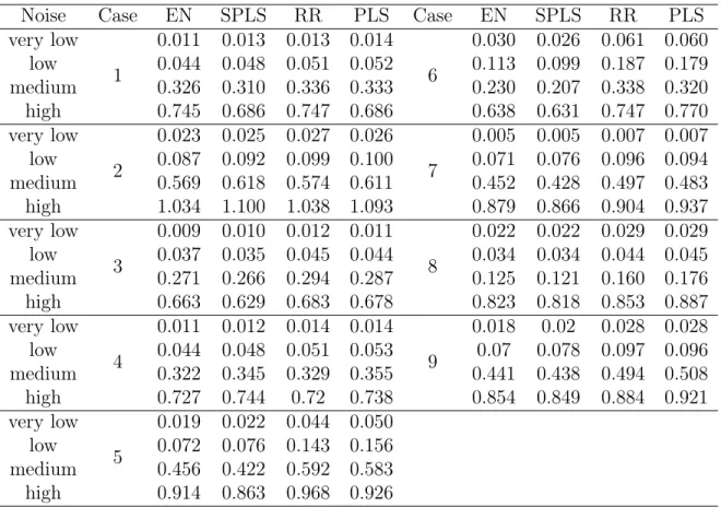
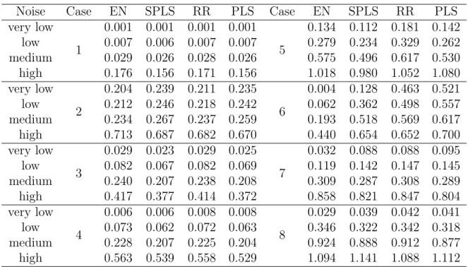
4.A Case study results for linear static method comparisons . . . 131
4.A.1 Type I cases: number of features < number of training samples 131 4.A.2 Type II cases: number of features > number of training samples 135 4.B Case study results for linear dynamic method comparisons . . . 137
4.B.1 Case 1 . . . 138
4.B.2 Case 2 . . . 139
4.B.3 Case 3 . . . 141
4.B.4 Case 4 . . . 142
4.B.5 Case 5 . . . 143
II
Advanced Process Monitoring
145
5 Introduction to Advanced Process Monitoring 147 5.1 Methodology for Fault Detection . . . 1495.2 Methodology for Fault Identification . . . 152
5.3 Methodology for Fault Classification . . . 154
5.4 Benchmark Dataset: TEP . . . 156
5.5 Summary of Contributions in Part II . . . 158
6 A Comparison Study of Different Fault Detection and Classifica-tion Strategies 161 6.1 Introduction . . . 161
6.2 Strategies in Which All Faults are Known . . . 163
6.2.2 Example 2: two-dimensional space with fault detectable in
pro-jected space . . . 167
6.2.3 Example 3: two-dimensional space with fault detectable in residual space . . . 171
6.2.4 General case with projection . . . 174
6.3 Strategies with Unknown Faults . . . 176
6.3.1 Example 1: one-dimensional space without projection . . . 177
6.3.2 Examples 2 and 3: two-dimensional space with fault detectable in either projected space or residual space . . . 180
6.4 Conclusion . . . 182
7 Probabilistic PCA for Multivariate Process Monitoring 185 7.1 Introduction . . . 185
7.2 PPCA-based Fault Detection . . . 187
7.2.1 PPCA Algorithm . . . 187
7.2.2 Fault Detection . . . 188
7.2.3 Reduction Order . . . 190
7.3 Theoretical Justification of PPCA . . . 192
7.4 Comparisons Between PPCA and PCA . . . 195
7.4.1 Advantages of PPCA over PCA . . . 195
7.4.2 The Projection Difference Between PPCA and PCA . . . 197
7.4.3 Computational Complexity . . . 198
7.4.4 The Relationship Between PPCA-based and PCA-based Mon-itoring Statistics . . . 198
7.5 Case Study . . . 202
7.6 Conclusion . . . 206
8 Concurrent Canonical Variate Analysis for Process Quality and Dynamic Monitoring 207 8.1 Introduction . . . 207
8.2.1 CVA Theorem . . . 209
8.2.2 Standard CVA for Process Monitoring . . . 210
8.3 PQDM Methodology . . . 211
8.3.1 CCVA for Quality Monitoring . . . 212
8.3.2 Dynamic Monitoring . . . 216
8.4 Implementation Scheme for PQDM . . . 217
8.5 Case Studies . . . 219
8.5.1 Fault 4: Step Change in Reactor Cooling Water Inlet Temperature219 8.5.2 Fault 11: Random Variation in Reactor Cooling Water Inlet Temperature . . . 221
8.6 Conclusion . . . 222
8.A Comparison of Different Adaptive Fault Detection Methods . . . 223
9 An Information-theoretic Framework for Fault Detection Evalua-tion and Design of Optimal Dimensionality ReducEvalua-tion Methods 229 9.1 Introduction . . . 229
9.2 Method . . . 231
9.2.1 Evaluation framework for the fault detection problem . . . 231
9.2.2 Fault Detection Evaluation by Information Methods . . . 233
9.3 Case Study . . . 237
9.4 Conclusion . . . 240
9.A Proof of Lemma 9.2.1 . . . 241
9.B Proof of Lemma 9.2.2 . . . 243
10 Maximum Entropy Analysis for Feature Extraction in Process Monitoring 245 10.1 Introduction . . . 245
10.2 Principal of Maximum Entropy . . . 246
10.2.1 Maximum Entropy as the Optimal Feature Extraction Method 247 10.2.2 Comparison with PCA . . . 249
10.3.1 Realization of MEA Based on Renyi’s Entropy . . . 250
10.3.2 Algorithm of MEA . . . 251
10.3.3 Convergence and Computational Cost Analysis . . . 254
10.4 Online Monitoring Strategy of MEA . . . 255
10.5 Case Study . . . 257
10.5.1 Fault 2: Step Change in B Composition . . . 258
10.5.2 Fault 10: Random Variation in C Feed Temperature . . . 259
10.5.3 Overall Results for 20 Predefined Faults . . . 260
10.6 Conclusion . . . 261
11 Mutual Information Analysis for Feature Extraction in Process Monitoring 263 11.1 Introduction . . . 263
11.2 The MI Theorem . . . 265
11.2.1 MIA as the optimal lower dimensional linear model for prediction265 11.2.2 MIA of the State-space Model . . . 268
11.3 MIA for Process Monitoring . . . 270
11.3.1 Quadratic MI as an Estimator for MIA Computation . . . 270
11.3.2 Algorithm for MI Modeling . . . 273
11.3.3 MIA Statistics for Fault Detection . . . 274
11.4 Discussions on the Relationship Between MIA and CVA . . . 275
11.5 Application to the TEP . . . 276
11.5.1 Fault 9: Random Variation in D Feed Temperature . . . 277
11.5.2 Fault 3: Step Change in D Feed Temperature . . . 280
11.5.3 Results of 20 Predefined Faults . . . 281
11.6 Conclusion . . . 282
11.A Proof of Theorem 11.2.1 . . . 283
11.B Approximation of Shannon’s MI . . . 283
11.B.1 Property 1: Invariant under Invertible Transformation . . . . 284
11.C Proof of the Discussion in Section 11.4 . . . 287
12 Feature Extraction for Fault Classification Based on Maximizing Jensen-Shannon Divergence 289 12.1 Introduction . . . 289
12.2 JSD Revisited . . . 291
12.3 JSD-based Feature Extraction for Classification . . . 293
12.3.1 Bayes Error Viewpoint for JSD-based Feature Extraction . . . 293
12.3.2 Bayesian Inference Interpretation for JSD-based Feature Ex-traction . . . 294
12.4 Method of MJDA for Gaussian Classes . . . 296
12.5 Application to the TEP . . . 299
12.6 Extension to General Distributions . . . 302
12.7 Conclusion . . . 306
13 Review and Comparative Study of Nonlinear PCA Fault Detection Methods 307 13.1 Introduction . . . 307
13.2 General ways of building nonlinear models . . . 310
13.3 NPCA Based on Feature Transformation: KPCA . . . 311
13.3.1 Background on Kernel Methods . . . 312
13.3.2 KPCA . . . 313
13.4 NPCA Based on Local Linear Approximation: LLE . . . 318
13.4.1 LLE . . . 319
13.4.2 Discussion of Limitations of LLE for Process Monitoring . . . 327
13.5 NPCA Based on Feature Transformation and Function Approximation: NN-NPCA . . . 328
13.5.1 Background of NNs . . . 328
13.5.2 ANN . . . 330
13.5.3 Principal Curves and NN-based NPCA . . . 336
13.6 Other NPCA Methods . . . 343
13.6.1 Principal Curves . . . 343
13.6.2 GP . . . 344
13.6.3 Probabilistic NPCA . . . 345
13.6.4 Hebbian Networks . . . 348
13.7 Selection of the Number of PCs . . . 348
13.7.1 Selection Based on NOC Data . . . 349
13.7.2 Selection Based on the Fault Information . . . 351
13.7.3 Comments . . . 352
13.8 Nonlinearity Assessment . . . 353
13.8.1 Quadratic Test . . . 354
13.8.2 Maximal Correlation Analysis . . . 355
13.8.3 Sufficiency of Nonlinearity Assessment . . . 356
13.9 Case Studies . . . 358
13.9.1 A simple linear example . . . 359
13.9.2 A Simple Nonlinear Example . . . 366
13.9.3 TEP . . . 373
13.9.4 Buffer Creation Process . . . 385
13.10Conclusion and Discussion . . . 399
13.10.1 Summary . . . 399
13.10.2 Conclusions . . . 400
13.10.3 Remarks . . . 400
13.10.4 Research Needs . . . 404
14 Fault Detection and Identification Using Bayesian Recurrent Neu-ral Networks 407 14.1 Introduction . . . 407
14.2 Background . . . 411
14.2.1 RNNs . . . 411
14.2.3 Variational Dropout as Bayesian Approximation . . . 415
14.3 Methodology for FDI . . . 418
14.3.1 Fault Detection . . . 419 14.3.2 Fault Identification . . . 423 14.3.3 FDI Scheme . . . 425 14.4 Case Studies . . . 426 14.4.1 TEP . . . 427 14.4.2 Real Dataset . . . 444 14.5 Conclusion . . . 450
Conclusion
452
15 Conclusion 453 15.1 Summary of Contributions . . . 45315.2 Challenges and Opportunities . . . 454
15.2.1 Experimental Design and Data Collection . . . 454
15.2.2 Utilizing New Information Streams . . . 455
15.2.3 Advanced process data analytical approaches . . . 456
Appendix
457
List of Figures
2-1 Illustration of a predictive modeling problem. . . 45 2-2 Plot of the contours of the non-regularized error function (blue) along
with the constraint region (red) for (a) LASSO 𝑞 = 1, (b) ridge regres-sion 𝑞 = 2, (c) elastic net, for a prediction model with two predictors. The figure is based on [1]. . . 49 2-3 Illustration of the PLS matrix decomposition. The loading matrices are
calculated to maximize the covariance between the score matrices. . . 50 2-4 Illustration of the SVR lost function. Only points outside the shaded
region contribute to the cost function. The left figure shows a linear SVR model, and the right figure shows a nonlinear SVR model with kernel function. . . 51 2-5 Illustration of a single regression tree. Each internal node tests a
par-ticular predictor 𝑥𝑖 and each leaf assigns an output value. . . 52
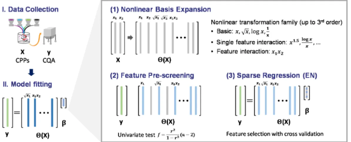
3-1 Schematic of the ALVEN algorithm. The three steps in ALVEN algo-rithm are (1) nonlinear basis expansion, (2) feature pre-screening via univariate test, and (3) sparse regression via the EN. . . 60 3-2 3D printer data visualization via single-variable histograms and scatter
plots: LH is the layer height, WT is the wall thickness, ID is the infill density, NT is the nozzle temperature, BT is the bed temperature, PS is the print speed, M is the material, FS is the fan speed, and TS is the tension strength. . . 65
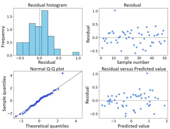
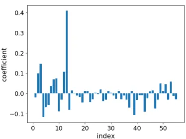
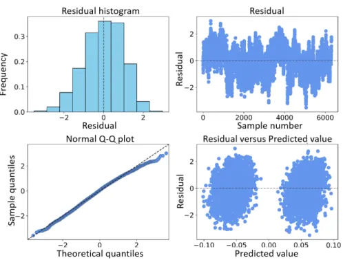
3-3 Testing error distributions via nested cross-validation for the 3D printer dataset by three different nonlinear modeling methods. . . 66 3-4 Model prediction results for ALVEN for a 3D printer. . . 67 3-5 Residual analysis for the ALVEN model of the 3D printer. . . 68 3-6 Model coefficients for the final retained terms in the ALVEN model for
a 3D printer. . . 69 3-7 CSTR data visualization as single-variable histograms and scatter plots:
Q is the coolant flow rate and CA is the concentration of A. . . 69 3-8 Training MSE for the CSTR data over 10 prediction steps. . . 70 3-9 Testing MSE for the CSTR data over 10 prediction steps. . . 70 3-10 CSTR 1-step ahead prediction result for the testing data by
DALVEN-full (AIC). . . 71 3-11 Model coefficients for the final retained terms in the DALVEN-full
(AIC) model of the CSTR. . . 71 4-1 Systematic data interrogation procedure for predictive modeling. . . . 75 4-2 The data analytics triangle for predictive modeling with a single
re-sponse variable. The modeling techniques are mapped to three ma-jor model regression characteristics. ALVEN, algebraic learning via elastic net; CVA, canonical variate analysis; DALVEN, dynamic AL-VEN; MOESP, multivariable output error state space; PLS, partial least squares; RF, random forest; RNN, recurrent neural network; RR, ridge regression; SVR, support vector regression. References to the methods are given in the text. . . 76 4-3 Testing performance of four types of models. The curve shows the
median of testing MSEs over 3000 repetitions for each noise level: The unbiased model is quartic. The biased model is quadratic. The “cv” refers to selecting the order from 1 to 10 in a polynomial based on 3-fold cross-validation. The “cv limited order” refers to selecting the order from 2 and 4 in a polynomial based on 3-fold cross-validation. . . 77
4-4 Testing prediction error variation for the four types of models. Each curve is the median of the standard deviation of testing MSEs over 3000 repetitions for each noise level. Plot (b) is a zoomed version of plot (a) to resolve the performance difference between the unbiased model, biased model, and cross-validation with limited order. . . 80 4-5 Median MSE for the four methods for two cases in Type I: Case 2 and
Case 5 with high noise level. . . 92 4-6 Median MSE for the four methods with different noise levels of Case 1
in Type I. . . 93 4-7 Median MSE for the four methods for Case 8 in Type II. . . 93 4-8 Median MSE for the four methods for Case 1 and its sparse version
Case 5 in Type I. . . 93 4-9 RNN with feedback and one state layer for predictive modeling. . . 102 4-10 Multi-step (3-step in this example) prediction by RNN with feedback
correction and one state layer. . . 102 4-11 Illustration of 𝑘-fold cross-validation (𝑘 = 5). . . 104 4-12 Illustration of Monte Carlo-based cross-validation with 5 repetitions. . 105 4-13 Illustration of leave-one-group-out cross-validation. . . 106 4-14 Illustration of nested cross-validation, using 𝑘-fold cross-validation as
an example. The conventional cross-validation will just select one held-out dataset as a test dataset, whereas nested cross-validation repeats the procedure using the outer loop. . . 107 4-15 Illustration of the one-standard-error rule. The conventional
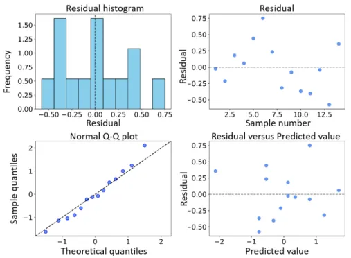
cross-validation will select 5 as the number of latent variables while the one-standard-error rule will pick 3 as the final latent variables. . . 108 4-16 Illustration of time-series cross-validation with 3 folds. . . 108 4-17 Fiber data visualization: single-variable histograms and scatter plots. . 110 4-18 Nonlinearity test results for the fiber data. . . 111 4-19 Comparison of raw fiber data with predictions from the OLS model. . 112 4-20 Residual analysis for the OLS model of the fiber data. . . 112
4-21 Example ATR-FTIR spectra for KDP solution: (left) raw spectra, (right) identified blue regions with spectral artifacts that should be
removed in pre-processing. . . 113
4-22 Absorbance at wavenumber 1074.17 cm−1 of KDP solutions at differ-ent temperatures (label corresponds to KDP concdiffer-entration). This fre-quency corresponds to the peak absorbance, which makes it easier to evaluate trends due to having the highest signal-to-noise ratio. . . 114
4-23 Sparse regression results for spectral data for (left) SPLS and (right) EN for the original dataset: the blue line is the average spectra over 116 samples while the red line shows the final model parameters for the absorbances. . . 116
4-24 PLS model prediction results by (left) PLS with standard cross-validation strategy and (right) SPA. . . 117
4-25 Scatterplot of CCPP data using 200 training data points. The breadth of scatter in the predictor variables indicate that the data reasonably cover the input space. . . 118
4-26 Nonlinear test results for CCPP data. One of the values is much greater than 1. . . 119
4-27 Multicollinearity test results for CCPP data. . . 120
4-28 CCPP model predictions vs. testing data for the SVR model using 200 training data points. . . 121
4-29 CCPP residual analysis for testing data. . . 122
4-30 Water evaporator data for the three input variables (FF, VF, and CF) and one output variable (DM). . . 123
4-31 Water evaporator data scatter plot. . . 124
4-32 Nonlinearity test for water evaporator data. . . 125
4-33 Multicollinearity test for water evaporator data. . . 125
4-34 Comparison of model predictions and raw testing data for a static linear model of a water evaporator. . . 126
4-35 Residual analysis for the testing data for a static linear model of a water evaporator. . . 127 4-36 Autocorrelation analysis for the residuals for the testing data for a static
linear model of a water evaporator. . . 127 4-37 Dynamic nonlinearity tests for the water evaporator data. . . 128 4-38 Testing prediction MSE for water evaporator data for seven data
ana-lytics methods for 0 to 10 prediction steps. . . 128 4-39 Comparison of predicted values with testing data for an SSARX model
for a water evaporator. . . 129 4-40 Water evaporator SSARX model residual analysis for testing data. . . 130 4-41 Water evaporator SSARX model residual dynamic analysis for testing
data. . . 130 4-42 Type I case testing MSE distributions for RR, PLS, EN, SPLS, and
OLS with all predictors/only useful predictors. . . 133 4-43 Type I case: testing MSE medians with 95% confidence interval for RR,
PLS, EN, and SPLS. . . 134 4-44 Type II case: testing MSE distributions for RR/PLS/EN/SPLS and
RR/PLS with only useful predictors. . . 136 4-45 Type II case: testing MSE medians with 95% confidence interval for
RR, PLS, EN, and SPLS. . . 137 4-46 Case 1 data for linear dynamic model comparison. . . 138 4-47 𝑘-step ahead prediction MSE results for Case 1 testing set by
differ-ent methods with 400 training samples. The label ‘auto’ indicates the option for automatic algorithm selection in N4SID in Matlab, which selects the weights in the subspace algorithm from MOESP, CVA, and SSARX. . . 138 4-48 𝑘-step ahead prediction MSE results for Case 1 testing set by different
methods with 300 training samples. . . 139 4-49 Case 2 data for linear dynamic model comparison. . . 140
4-50 𝑘-step ahead prediction MSE results for Case 2 testing set by different methods with 400 training samples. . . 140
4-51 𝑘-step ahead prediction MSE results for Case 2 testing set by different methods with 300 training samples. . . 141
4-52 Case 3 data for linear dynamic model comparison. . . 141
4-53 𝑘-step ahead prediction MSE results for Case 3 testing set by different methods. . . 142
4-54 Case 4 data for linear dynamic model comparison. . . 142
4-55 𝑘-step ahead prediction MSE results for Case 4 testing set by different methods. . . 143
4-56 Case 5 data for linear dynamic model comparison. . . 143
4-57 𝑘-step ahead prediction MSE results for Case 5 testing set by different methods. . . 144
5-1 Process monitoring loop [2] . . . 147
5-2 Illustration of PCA decomposition. The original data matrix 𝑋 is decomposed into the principal subspace and the residual space. . . 150
5-3 Illustration of fault detection indices for the specific case of three vari-ables with one principal component. The projection space is a one-dimensional space depicted as the dashed line in the figure. The 𝑇2
statistic measures the variation of the data projection onto that line, and defines a specific region by two planes in the original space. Any data points that fall between those two planes are considered as be-ing normal by the 𝑇2 statistic. The control limit for the distance of the
data points to the projection space is specified by the 𝑄 statistic. In this example, √𝑄 is the shortest distance between any point to the dashed line, which in this case denotes a cylinder of the in-control region. More generally, the shape of the NOC defined by the combination of the 𝑇2
and 𝑄 statistics is the intersection of the interior of a hyperellipsoid in one subspace and the interior of a hyperellipsoid in the complementary subspace. . . 153 5-4 A process flowsheet for the TEP with the second control structure in [3].158 6-1 Different strategies for fault detection and classification without
un-known classes. . . 163 6-2 Different layouts for classes in Example 1. . . 164 6-3 Region distributions for layout 1 in Example 1. Boundaries between
different regions are shown in the lower part of the corresponding figures.165 6-4 Region distributions for layout 2 in Example 1 with different significance
levels. Boundaries between different regions are shown in the lower part of the corresponding figures. . . 168 6-5 Different layouts for classes in Example 2. For layout 1: 𝜇0 = [0, 0]⊤,
𝜇1 = [3, 3]⊤,𝜇2 = [12, 6]⊤; for layout 2: 𝜇0 = [0, 0]⊤, 𝜇1 = [−3, −3]⊤,
𝜇2 = [12, 6]⊤. . . 169
6-6 Illustration of fault detection and classification boundaries in Example 2 layout 1. . . 170
6-7 Region distributions for layout 1 in Example 2 with different significance levels. . . 171 6-8 Region distributions for layout 2 in Example 2 with different significance
levels. . . 172 6-9 Different layouts for classes in Example 3. Three classes have different
means: 𝜇0 = [0, 0]⊤, 𝜇1 = [−2, 1]⊤,𝜇2 = [6, 6]⊤. . . 173
6-10 Region distributions for Example 3 with different significance levels. . 175 6-11 Nine different strategies for situations with data from unknown faults. 178 6-12 Illustration of possible active boundaries for Example 1 with nine
dif-ferent strategies. . . 179 6-13 Region distributions by nine different strategies for Example 1 layout
1. Case i-j represents strategy i with method j for outlier detection. . . 179 6-14 Region distributions by nine different strategies for Example 1, layout
2. Case 𝑖-𝑗 represents strategy 𝑖 with method 𝑗 for outlier detection. . 180 6-15 Region distributions by nine different strategies for Example 2. Case
𝑖-𝑗 represents strategy 𝑖 with method 𝑗 for outlier detection. . . 181 6-16 Region distributions by nine different strategies for Example 3. Case
i-j represents strategy i with method j for outlier detection. . . 182 7-1 Monitoring boundaries by (a) PCA and (b) PPCA for a two-dimensional
space. . . 199 8-1 Flowchart of the PQDM fault detection. . . 218 8-2 PQDM-based monitoring results for a step change in the reactor cooling
water inlet temperature. . . 220 8-3 CVA-based monitoring results for a step change in the reactor cooling
water inlet temperature. . . 220 8-4 PQDM-based monitoring results for a random variation in the reactor
cooling water inlet temperature. . . 221 8-5 CVA-based monitoring results for a random variation in the reactor
8-6 Adaptive fault detection flowchart. . . 223 8-7 Fault detection by PCA-based methods for NOC testing data. . . 225 8-8 Fault detection by PLS-based methods for NOC testing data. . . 226 9-1 Fault detection problem. . . 230 9-2 Shannon’s information theory problem [4,5]. . . 230 9-3 Information-theoretic formulation of fault detection. . . 234 9-4 Squared residuals for fault detection methods with optimal
transforma-tion for a single simulatransforma-tion: left with PCA and right with CVA. . . 238 9-5 Squared residuals for fault detection methods with random
transforma-tion for a single simulatransforma-tion: left with PCA and right with CVA. . . 239 9-6 The FDR and MI for PCA and CVA averaged over 1000 simulations. . 240 10-1 The monitoring statistics for Fault 2. . . 258 10-2 The monitoring statistics for Fault 10. . . 260 10-3 FDRs for 20 predefined faults by MEA and PCA. . . 261 11-1 FDRs at different orders for Fault 9. . . 278 11-2 Fault detection statistics for Fault 9 at 𝑘 = 18 (left is MIA and right is
CVA). . . 279 11-3 FDRs at different orders for Fault 3. . . 280 11-4 Fault detection statistics for Fault 3 at 𝑘 = 17 (left is MIA and right is
CVA). . . 281 11-5 FDRs for 20 predefined faults by MIA and CVA (𝑘 = 18). . . 282 12-1 The linear transformation of Fault 3, 4 and 11 onto the first two loading
vectors by (a) PCA, (b) DPLS, (c) FDA, and (d) MJDA. . . 300 12-2 The classification results for Faults 3, 4, and 11 obtained by (a) PCA,
(b) DPLS, (c) FDA, and (d) MJDA. The left axis labels the fault that occurs starting at time 𝑡 = 0, and the legend at the right gives the color of the fault indicated by the fault classification method. . . 302
12-3 Training data from Fault 1 (blue) and 2 (red). The first loading vectors by PCA, FDA, and MJDA are also shown on the figure. . . 305 13-1 Three general ways of building nonlinear model: (a) original nonlinear
relationship; (b) nonlinear feature transformation; (c) nonlinear approx-imation; (d) feature transformation and nonlinear approximation. . . . 310 13-2 A typical structure of a feedforward NN. . . 329 13-3 The ANN structure. . . 331 13-4 Principal curve and NN based NPCA structure. . . 338 13-5 ITN structure. . . 340 13-6 GP-based NPCA algorithm (note: the figure is based on [6]). . . 345 13-7 Two-dimensional manifold embedded in a three-dimensional space: (a)
linear subspace; (b) and (c) nonlinear submanifold (image adapted from [7]). . . 353 13-8 Example of the quadratic test unable to detect nonlinearity: (a)
sinu-soidal data, (b) 𝑝-values from quadratic tests, and (c) maximal corre-lations. . . 357 13-9 Example of the maximal correlation analysis unable to detect
nonlinear-ity: (a) nonlinear manifold by the bilinear term, (b) linear correlations, (c) 𝑝-values from quadratic tests, and (d) maximal correlations. . . 357 13-10 NOC data and faulty data of the simple linear example. . . 359 13-11 Linearity assessment for the simple linear example: (a) linear
correla-tion matrix of the NOC data; (b) scatter plot of the NOC data. . . 360 13-12 Nonlinearity assessment results for the simple linear example: (a)
𝑝-values from quadratic tests; (b) maximal correlations. . . 361 13-13 Parallel analysis results of (a) PCA; (b) KPCA-RBF; (c) KPCA-poly;
and (d) ANN for the simple linear example. . . 362 13-14 Monitoring charts of Fault 1 for the simple linear example. . . 363 13-15 Monitoring charts of Fault 2 for the simple linear example. . . 364 13-16 NOC data and faulty data of the simple nonlinear example. . . 367
13-17 Linearity assessment for the simple nonlinear example: (a) linear cor-relation matrix of the NOC data; (b) scatter plot of the NOC data. . . 368 13-18 Nonlinearity assessment results for the simple nonlinear example: (a)
𝑝-values from quadratic tests; (b) maximal correlations. . . 368 13-19 Parallel analysis results of (a) PCA; (b) KPCA-RBF; (c) KPCA-poly;
and (d) ANN for the simple nonlinear example. . . 369 13-20 Monitoring charts of Fault 1 for the simple nonlinear example. . . 370 13-21 Monitoring charts of Fault 2 for the simple nonlinear example. . . 371 13-22 Linear correlation matrix of the TEP. . . 374 13-23 𝑝-values of TEP NOC data by the quadratic test. . . 375 13-24 Maximal correlation matrix of TEP. . . 376 13-25 Scatter plot of TEP NOC data. . . 377 13-26 MDRs with different numbers of PCs by different methods for the TEP. 380 13-27 Diagram of the buffer make-up system. . . 385 13-28 Model of a single in-line mixer. . . 386 13-29 NOC data for the buffer creation process. . . 387 13-30 Linear correlation matrix for the buffer creation process. . . 389 13-31 𝑝-values from quadratic tests for the buffer creation process. . . 390 13-32 Maximal correlation matrix for the buffer creation process. . . 390 13-33 Scatter plot of the buffer creation process. . . 391 13-34 MDRs with different numbers of PCs by different methods for the buffer
14-1 A simple RNN structure with one recurrent layer and showing the un-folding in time of the sequence of its forward computation. The RNN includes the input variable 𝑥𝑡, state variable 𝑠𝑡 and outputs ˆ𝑦𝑡. The
state variable 𝑠𝑡 is calculated based on the previous state 𝑠𝑡−1 and the
current input 𝑥𝑡. The RNN output ˆ𝑦𝑡 is then calculated based on the
current state. In this way, the input sequence 𝑥𝑡 is mapped to output
sequence ˆ𝑦𝑡 with each ˆ𝑦𝑡 depending on all previous inputs. The model
parameters 𝜔 = {𝑊𝑠, 𝑈𝑠, 𝑊𝑠, 𝑏𝑠, 𝑏𝑦} are shared at each time step. . . 412
14-2 Illustration of the variational dropout technique (right) compared to standard dropout technique (left) for a simple RNN. Each graph shows units unfolded over time, with the lower level for inputs, middle level for state units, and upper level for output units. Vertical arrows represent the connections from inputs to outputs while horizontal arrows sent recurrent connections. The arrows with dashed grey lines repre-sent the standard connection without dropout. Colored lines reprerepre-sent dropout connections with different colors for different dropout masks. (Left) In the standard dropout technique, no dropout is applied for the recurrent layers, while other connections have different dropout masks at different time steps. (Right) For the variational dropout approach proposed in [8], dropout is applied to both input, recurrent, and output layers with the same dropout mask at different time steps. Variational dropout is applied during both training and testing. . . 416
14-3 General procedure for process monitoring system development (left) versus procedure for developing BRNN-based FDI system (right). The general framework to establish a monitoring system begins with a model to characterize NOC behavior, such as using the BRNN model to learn the NOC pattern from the training data. Then, the method to measure the deviation of a particular observation to the NOC region is chosen. In our case, the process observations are compared to the BRNN posterior predictive distributions. Finally, the decision will involve determining whether the acquired observation is from the NOC or not (i.e., compare deviations of observations for fault detection and assess which variables significantly deviate from the NOC for identification). . . 418
14-4 Depiction of BRNN model using variational dropout (left) for FDI. The BRNN model uses the current observation and state to predict the next system observation. The BRNN model is unrolled in two dimensions (right): the time of the computation involved in its forward computation and the stochastic repetition by variational dropout. At each time step, stochastic variational dropout is applied 𝑁 times and the corresponding MC prediction samples {ˆ𝑥𝑡(𝑖)}𝑖=1,...,𝑁 are used to
approximate the posterior predictive distribution for that time step. For the next time step, the same procedure is repeated and MC samples { ˆ𝑥𝑡+1(𝑖)}𝑖=1,...,𝑁 are collected and used to approximate the distribution. 420
14-5 Flowchart of the BRNN-based FDI methodology. The offline training stage (left) and the online monitoring stage (right) are shown in the figure. The procedure starts with offline training, and then the offline-trained model is used during online monitoring. The choice of statistics for detection and identification is made at design time. . . 426
14-6 BRNN model outputs for TEP NOC training data. The plot shows all 52 variables in TEP. The dark blue lines are the TEP measurements and the light blue lines correspond to the BRNN model predictive distribu-tion outputs for the NOC data. For measurements under the NOC, the dark blue lines should lie within the predictive distribution. . . 430 14-7 BRNN model outputs for TEP NOC validation data. . . 431 14-8 BRNN model outputs for TEP Fault 3. . . 434 14-9 Fault identification plot of the BRNN-𝐷𝑙 statistic for Fault 3. The
{︀𝐷𝑙}︀
𝑙=1,...,52 values for the 960 timesteps are color coded in the
identifi-cation plot. Variables with dark blues have high values of 𝐷𝑙, meaning
that the variable has positively deviated from the NOC region. Con-versely, variables with dark red have low values of 𝐷𝑙 and have
nega-tively deviated from the NOC region. A light color means the variable is not significantly affected by the disturbance. As expected, no variable significantly deviates from the NOC. . . 435 14-10 Contribution plots for Fault 3 from (a) r-PCA, (b) f-PCA, (c) r-DPCA,
and (d) f-DPCA. The plot shows the contribution factor and with the darkness of the blue color indicating the amount of deviation of the variable from the NOC region. . . 436 14-11 BRNN model outputs for TEP Fault 5. . . 437 14-12 Fault identification plot by BRNN-𝐷𝑙 for Fault 5. The switch between
dark blue and red colors shows that the system is undergoing large fluctuation. . . 438 14-13 Contribution plots for Fault 5 from (a) r-PCA, (b) f-PCA, (c) r-DPCA,
and (d) f-DPCA. . . 439 14-14 BRNN model outputs for TEP Fault 1. . . 441 14-15 Fault identification plot by BRNN-𝐷𝑙 for Fault 1. The root cause for
this uncontrollable fault can be assessed by looking at the variables that are persistently off the NOC region. . . 442
14-16 Contribution plots for Fault 1 from (a) r-PCA, (b) f-PCA, (c) r-DPCA, and (d) f-DPCA. . . 443 14-17 Sorted fault identification plot according to the detected deviation
oc-currence time of BRNN-𝐷𝑙 for Fault 6. . . 444
14-18 Fault 6 propagation path at the 180th data point (1 hour after the fault
occurs). Colored nodes indicate that the corresponding variable has been detected as deviating significantly from the NOC. . . 445 14-19 FDI by the BRNN model on the Fault 1 testing data. The red box
indicates the period with the foaming event recorded by the operator. 446 14-20 FDI by (D)PCA methods for Fault 1: (a) PCA, (b) f-PCA, (c)
r-DPCA, and (d) f-DPCA. The red box indicates the period with the foaming event recorded by the operator. . . 447 14-21 FDI by BRNN for Fault 2. The red box indicates the period with the
foaming issue as recorded by the operator. . . 448 14-22 FDI by (D)PCA methods for Fault 2: (a) PCA, (b) f-PCA, (c)
r-DPCA, and (d) f-DPCA. The red box indicates the period with the foaming issue as recorded by the operator. . . 449
List of Tables
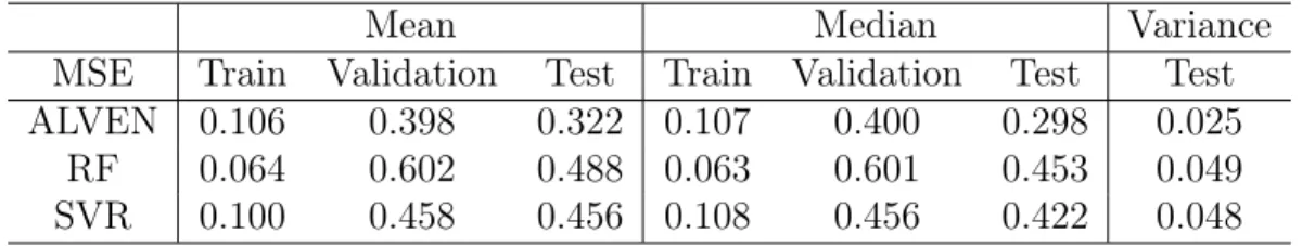
3.1 Model fitting results for 3D printer data using nested cross-validation. 66 4.1 Median MSE of testing data by multicollinearity methods for Type I
cases. . . 91 4.2 Median MSE of testing data by multicollinearity methods for Type II
cases. . . 92 4.3 Model prediction results for fiber data. . . 111 4.4 Mean squared errors for different static regression methods for CCPP
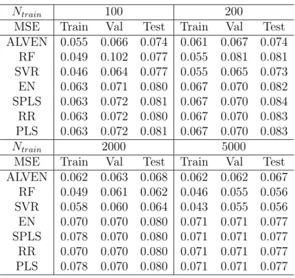
data with different numbers of training samples. . . 120 6.1 Monitoring results for layout 1 in Example 1 for three strategies [%]. . 167 6.2 Monitoring results for layout 2 in Example 1 for three strategies [%]. . 167 6.3 Monitoring results for layout 1 in Example 2 by three strategies [%]. . 170 6.4 Monitoring results for layout 2 in Example 2 by three strategies [%]. . 173 6.5 Monitoring results for Example 3 from the three strategies [%]. . . 174 6.6 Probability of the assigned region belongs to the corresponding class
[%] for Example 1, layout 1. . . 179 6.7 Probability of the assigned region belongs to the corresponding class
[%] for Example 1, layout 2. . . 180 7.1 FDRs by PCA and PPCA for the TEP [%]. . . 204 7.2 FDRs by PCA with 50/51 PCs [%]. . . 205 8.1 Monitoring statistics and detection thresholds of PQDM. . . 218 8.2 Adaptive fault detection FAR results [%]. . . 226
8.3 Adaptive fault detection FDR results [%]. . . 227 9.1 Fault detection performances. . . 239 12.1 MCRs for Fault 3, 4 and 11 by different methods. . . 301 12.2 MCRs by PCA, FDA, and MJDA for general distributions. . . 305 13.1 MDRs [%] for the simple linear example with parallel analysis/intrinsic
dimensionality for order selection. . . 363 13.2 MDRs [%] of the simple linear example with different numbers of PCs. 365 13.3 MDRs [%] of simple nonlinear example with parallel analysis/intrinsic
dimensionality for order selection. . . 370 13.4 MDRs [%] for simple nonlinear example with different numbers of PCs 372 13.5 MDRs [%] of TEP by different methods. . . 378 13.6 MDRs [%] of ANN with different numbers of hidden neurons for the TEP.381 13.7 MDRs [%] of KPCA-RBF with different kernel width for the TEP. . . 383 13.8 MDRs [%] of LLE with different numbers of 𝑘NN for the TEP. . . 384 13.9 Process faults of the buffer creation process. . . 388 13.10 MDRs [%] for the buffer creation process by different methods. . . 392 13.11 MDRs [%] of ANN with different numbers of hidden neurons for the
buffer creation process. . . 396 13.12 MDRs [%] of KPCA-RBF with different kernel width for the buffer
creation process. . . 398 13.13 MDRs [%] of KPCA-poly with different orders for the buffer creation
process. . . 398 13.14 MDRs [%] of LLE with different numbers of 𝑘NN for the buffer creation
process. . . 399 14.1 TEP fault detection percentage results. The FAR is shown for the NOC
Chapter 1
Introduction
1.1
Thesis goals
The unifying aim of this thesis is to develop advanced data analytics tools for man-ufacturing processes. Data analytics is playing an increasingly important role in next-generation manufacturing processes for improving process productivity, reliabil-ity, and control [9–11]. Often in real manufacturing processes, the approach of using mathematical models based on first principles is unavailable or too time-consuming to apply due to the complexity of the systems. On the other hand, when sufficient data are available, data analytics methods can be applied at relatively low cost at many different scales, from individual sensors to unit operations to the entire manufacturing plants. Opportunities for process data analytics are further enabled by advances in sensor technology, wireless networks, and computational power, and the availability of low-cost data storage.
Despite major advances in machine learning and data science, the uptake of ad-vanced data analytics methods to real manufacturing processes has been relatively slow. One major reason is the complexity of real manufacturing processes. Real manufacturing systems often involve nonlinear multivariable interactions between the system variables. For fast-sampling processes, system dynamics are important for model construction. A real manufacturing process can also have time-varying op-erating conditions where the performance of any offline-trained model degrades over
time. The second reason is the diversity in data quantity and quality. While advances in sensor technology have created much more data for some manufacturing processes, it is very costly to acquire large amounts of data for other processes, and the data quality can be low because of sensor drift, bias, and noise and unmeasured distur-bances. The relatively limited use of advanced data analytics in real manufacturing processes and the wide variety of available methods calls for a systematic review and guidelines on how to select the best-in-class method for a given application, how to correctly construct the model, and how to interpret the results.
This thesis explores ways to address the above challenges with an emphasis on two application areas: predictive modeling and process monitoring. Besides the de-velopment of advanced algorithms, this thesis also addresses the importance of using a systematic framework for data analysis and points out common misconceptions in the literature and industry. The next section describes the objectives of this thesis in more detail.
1.2
Thesis organization
Chapters 2–4 considers process data analytics methods for application to predictive modeling.
• Chapter 2 describes basic concepts of regression and provides an introduction to popular regression techniques.
• Chapter 3 introduces a new technique for interpretable nonlinear model con-struction. The proposed approach combines automated feature generation for chemical and biological processes and a two-step sparsity-promoting regression procedure, which produces an interpretable nonlinear model. The proposed technique can be extended to dynamic nonlinear model construction. The in-terpretability sheds light on the physical properties of the process, and more importantly, it can be easily integrated with other application purposes, such as control/optimization design. The proposed methods are tested in two case
stud-ies, which show robust and accurate performance over state-of-the-art black-box nonlinear models.
• Chapter 4 presents a systematic approach for automated and robust method selection and model construction for manufacturing processes, which empowers the users to focus on goals rather than on methods and automatically trans-forms manufacturing data into intelligence. The focus of the framework is on predictive modeling, and the general framework can be applied to other ap-plications. For automated method selection, a bottom-up approach is taken to select the best-in-class method based on the characteristics of the data and available domain knowledge. For automated model construction, the appro-priate cross-validation strategy is selected based on data attributes and rigor-ously implemented to validate model performance. The proposed framework is demonstrated on several case studies with different data characteristics, includ-ing nonlinearity, multicollinearity, and dynamics.
Chapters 5—14 considers process data analytics for application to process monitoring, which separately address specific key challenges encountered in real manufacturing processes.
• Chapter 5 introduces basic concepts and methods for process monitoring, in-cluding fault detection, identification, and classification. Also, the benchmark dataset from the Tennessee Eastman process (TEP) is introduced, which is commonly used to test and compare process monitoring algorithms.
• Chapter 6 discusses the impact of fault detection and classification strategy on the final performance. For the case where data are all from known classes, three strategies for fault detection and classification are proposed, and com-parisons are drawn based on case studies. For the case of data from known and unknown classes, three approaches are proposed, and the combination with different strategies are investigated based on case studies. This work shows the importance of analyzing the process monitoring strategy.
• Chapter 7 proposes a probabilistic framework for optimal fault detection of Gaussian linear processes based on probabilistic principal component analysis (PPCA) with a novel monitoring index. The proposed probabilistic approach is fundamentally different from the widely applied principal component analysis (PCA) method. Moreover, the proposed PPCA framework enables the selection of the optimal number of principal components (PCs) based only on normal operating data. Detailed comparisons between PPCA and PCA are provided, which show the advantages of PPCA in terms of model accuracy, robustness, and generalization capability. The equivalency between the weighted combination of PCA-based monitoring indices and the PPCA-based monitoring index is also discovered. The proposed PPCA-based fault detection method is applied to the TEP and compared with PCA.
• Chapter 8 discusses the development of a self-learning fault detection system for time-varying normal operating conditions (NOCs). A self-learning system is proposed to inform when the monitoring model should be updated. The proposed system is developed based on concurrent canonical variate analysis (CCVA) and has three sets of monitoring indices for both quality and dynamic monitoring, which is capable of accurately distinguish the normal variation from a real fault. The online model update is only necessary when the system has a normal variation. The proposed system is tested on the TEP. Besides, a review and comparison study for various commonly used adaptive algorithms are provided in the appendix, illustrating the importance of online updates of fault detection models for the process with varying normal conditions.
• Chapters 9–13 present a unified information-theoretic learning framework for advanced fault detection and classification algorithm developments, which over-comes the limitation associated with traditional second-order statistical learning methods. The information-theoretic learning framework explores information beyond the second-order moment, which is important for non-Gaussian pro-cesses, as discussed in Chapter 9. Linear subspace learning methods are
de-veloped based on the information maximization principle. Renyi’s information definition combined with kernel density estimators has been applied in order to cope with the difficulties in mathematical formulations and computations by using Shannon’s definition. The developed algorithms can be viewed as generalizations of traditional statistical learning methods: (1) maximized en-tropy analysis as a generalization of PCA in Chapter 10, (2) mutual information analysis (MIA) for quality variable monitoring as a generalization of canonical variate analysis (CVA) in Chapter 11, and (3) maximized Jensen-Shannon di-vergence analysis (MJDA) for fault classification in Chapter 12. The proposed algorithms are tested on the TEP and compared with traditional statistical learning methods.
• Chapter 13 provides a systematic review and comparative study of nonlinear PCA (NPCA)-based fault detection methods. Different nonlinear extensions of PCA have been proposed in order to address the challenges with nonlinear sub-manifold learning. However, there has been no systematic review of the various NPCA methods, especially for fault detection purposes. A thorough discussion on assumptions, algorithms, fault detection schemes, strengths, and limitations of various NPCA algorithms is provided. Moreover, a systematic methodology for deciding when to use a nonlinear fault detection method is proposed based on data interrogation. The most widely studied NPCA methods for fault detection – including kernel PCA (KPCA), locally linear embedding (LLE), and neural network PCA (NN-NPCA) – are compared with PCA in several linear and nonlinear case studies that collectively illustrate significant limitations and strengths of various NPCA methods. In addition to pointing out some common misconceptions in the literature, the case studies are used to provide general guidelines on when to use NPCA, how to use NPCA effectively, and how to interpret the results for fault detection of nonlinear systems.
• Chapter 14 explores an application of Bayesian recurrent neural networks (BRNNs) for fault detection and identification (FDI). A newly developed deep learning
approach using BRNNs with variational dropout is adopted, which directly tack-les three key challenges in modeling real process data: nonlinearity, dynamics, and uncertainties. The proposed BRNN-based method provides robust fault detection of chemical processes, direct fault identification with higher accuracy and specificity, and visualized fault propagation analysis. The outstanding per-formance of this method is contrasted to (dynamic) PCA in the TEP and an industrial dataset from chemical manufacturing.
Chapter 15 concludes the thesis, discusses ongoing challenges, and provides additional ideas of future research needs for process data analytics.
Part I
Chapter 2
Introduction to Predictive Modeling
The objective of predictive modeling is to build mathematical models to estimate the relationships between the output (response) variable and the inputs (predictors) based on the training data. The purpose of the constructed model is to predict new or future observations, as depicted in Figure 2-1. The model can also improve understanding the process that generated the data, which is especially useful for manufacturing processes. For example, such models can inform on which are the key variables for affecting product quality, and to identify rate-limiting steps in the manufacturing process.
Figure 2-1: Illustration of a predictive modeling problem. The most basic predictive model has the form
𝑦 = 𝑓 (𝑥) + 𝜀 (2.1)
where 𝑦 represents a univariate response variable, 𝑥 ∈ R𝑚𝑥 is a vector of predictors,
Predictive modeling also includes temporal forecasting where observations of pre-dictors (and outputs, if needed) up to time 𝑡 are used to forecast the future values for the output at time 𝑡 + 𝑘, 𝑘 > 0.
Two steps are involved with predictive modeling: the model form 𝑓(·) needs to be selected, and then an appropriate learning algorithm needs to be picked to estimate the model. There are many types of regression models. The simplest linear static model is
𝑦 = 𝑤0+ 𝑤1𝑥1+ · · · + 𝑤𝑚𝑥𝑥𝑚𝑥 (2.2)
where 𝑤0, . . . , 𝑤𝑚𝑥 are the model parameters. The parameter 𝑤0 represents the
inter-cept of the regression model, which allows for any fixed offset. It is often convenient to define an additional dummy variable 𝑥0 = 1 so that
𝑦 = 𝑤⊤𝑥 + 𝜀 (2.3)
where 𝑤 = [𝑤0, . . . , 𝑤𝑚𝑥]
⊤
∈ R𝑚𝑥+1 is a vector of model parameters (aka weights).
The most basic way of reconstructing the model parameters in Equation 2.3 is via ordinary least squares (OLS), which minimizes the mean squared error (MSE) of the predictions, min 𝑤 1 𝑁 𝑁 ∑︁ 𝑖=1 (𝑦𝑖− 𝑤⊤𝑥𝑖)2 (2.4)
where 𝑁 is the total number of training data points, and 𝑖 is the index for a specific observation.
Given the training predictor matrix 𝑋 ∈ R𝑁 ×𝑚𝑥 and the training output vector
𝑦 ∈ R𝑁, OLS has a unique analytical solution ˆ
𝑤𝑂𝐿𝑆 = (𝑋⊤𝑋)−1𝑋⊤𝑦 (2.5)
provided that the matrix 𝑋⊤𝑋 is invertible.
The Gauss-Markov theorem states that OLS produces the best linear unbiased estimation under certain conditions. Those conditions include: (1) the underlying
relationship between the predictor variables 𝑥 and the output variable 𝑦 should be linear, (2) the design matrix 𝑋 has full rank (identification condition), and (3) errors are uncorrelated, homoscedastic, and have zero mean.
Alternatives are required when one or more of the assumptions are violated, which include: (1) nonlinear relationship between the output and predictors, (2) strong multicollinearity between predictors, (3) serial correlations in the model errors, which implies unexplained dynamics in the response, and (4) heteroscedasticity of the model errors. Moreover, in cases with a large number of predictors, OLS performs poorly in terms of model robustness and interpretation.
In the aforementioned situations, other predictive modeling techniques give more robust and accurate prediction results. For example, latent variable models and regularized regression techniques are suitable for data with multicollinearity. For nonlinear problems, support vector regression (SVR) and random forests (RFs) are powerful methods to approximate a nonlinear structure. For dynamical systems, system identification techniques, e.g., state-space models, can capture the dynamic information of the process. Introductions to these popular regression techniques are provided in next sections.
2.1
Linear Regression with Penalty
Regularized linear regression is formulated as a linear regression plus a penalty for model complexity, min 𝑤 ‖𝑦 − 𝑋𝑤‖ 2 2+ 𝜆‖𝑤‖ 𝑞 𝑞 (2.6)
where 𝜆 is a positive penalty coefficient that quantifies the relative tradeoff between the complexity of a model and its training error.
For different 𝑞, the penalty norm has different forms. If 𝑞 = 2, the formulation is ridge regression (RR) [12]. RR is useful for data with multicollinearity, and has a simple analytical solution,
ˆ
This solution is unique and the matrix inverse is well-defined for any 𝜆 > 0.
RR shrinks the norm of the model parameters, which gives a biased estimation in order to increase prediction accuracy through a bias-variance tradeoff. However, the shrinkage does not necessarily result in the removal of variables. Other values of 𝑞 could give more sparse models as compared to RR. If 𝑞 = 0, the penalty norm is called the 𝑙0 pseudonorm and is the number of nonzero regression coefficients.
This regression problem is also called best subset selection. The motivation for this formulation is to directly select the most useful features and provide an interpretable model.
The optimization that defines 𝑙0-regularization is NP-hard, inherently
combinato-rial, and computationally expensive to solve. The tightest convex relaxation of the 𝑙0
pseudonorm penalty is the 𝑙1 norm penalty. The sparse regression with the 𝑙1 norm
penalty is called least absolute shrinkage and selection operator (LASSO) [13], which also promotes sparsity. LASSO tends to select slightly more variables as compared to best subset selection, but is computationally efficient and has been successful in many applications. However, for datasets with a large number of variables 𝑚𝑥 > 𝑁
or highly correlated variables, LASSO has limited performance. The elastic net (EN) has been proposed to resolve the limitations associated with LASSO [14]. EN does feature selection and continuous shrinkage simultaneously, enabling variable selection with only limited data and can select groups of correlated variables. EN is formulated as
min
𝑤 ‖𝑦 − 𝑋𝑤‖ 2
2+ 𝜆(𝛼‖𝑤‖1+1−𝛼2 ‖𝑤‖22) (2.8)
where 𝛼 is a scalar between 0 and 1 which specifies the tradeoff between the 𝑙1 and
𝑙2 penalties.
The combination of 𝑙1 and 𝑙2 penalties imposes both sparsity and grouping effects,
which provides stable and automated feature selection with good prediction accuracy. The LARS-EN algorithm is proposed [14] to solve the EN efficiently, which is based on the LARS algorithm for LASSO and has computational advantages over other optimization techniques for feature selection.
Figure 2-2: Plot of the contours of the non-regularized error function (blue) along with the constraint region (red) for (a) LASSO 𝑞 = 1, (b) ridge regression 𝑞 = 2, (c) elastic net, for a prediction model with two predictors. The figure is based on [1].
The optimizations that define ridge regression, LASSO, and elastic net can be reformulated as equivalent optimizations in which the penalty terms move from the objective function to become constraints. Those formulations can be used to interpret the three methods geometrically [1]. For example, it is clear from inspection of Figure 2-2 why LASSO generates sparse solutions and why ridge regression does not, and how elastic net compromises between the other methods.
2.2
Partial Least Squares
Partial least squares (PLS) is a dimensionality reduction technique that maximizes the covariance between the predictor matrix 𝑋 and the output matrix 𝑌 ∈ R𝑁 ×𝑚𝑦
for each component in the lower dimensional space. PLS can extract latent variables for a single output variable 𝑚𝑦 = 1 or multiple output variables. When only a single
output variable is considered, PLS is also referred to as PLS1. There are different algorithms to solve PLS, all of which apply an iterative process to extract the latent variable in the lower dimensional space.
In each iteration, PLS computes loading and score vectors by successively extract-ing factors from both predictor matrix and predicted matrix such that the covariance between the extracted factors is maximized,
max 𝑙𝑖,𝑞𝑖 𝑙⊤𝑖 𝑋𝑖⊤𝑌𝑖𝑞𝑖 s.t. 𝑙⊤ 𝑖 𝑙𝑖 = 𝑞𝑖⊤𝑞𝑖 = 1 (2.9)
where 𝑙𝑖 and 𝑞𝑖 are the projection vectors for the matrices 𝑋 and 𝑌 , respectively.
PLS decomposes the 𝑋 and 𝑌 matrices into the score matrix 𝑇 ∈ R𝑁 ×𝑘 and
𝑈 ∈ R𝑁 ×𝑘 and the residual matrix 𝐸 ∈ R𝑁 ×𝑚𝑥 and 𝐹 ∈ R𝑁 ×𝑚𝑦, where 𝑘 is the
dimension of the lower dimensional space by projecting along the loading matrix 𝑃 ∈ R𝑚𝑥×𝑘 and 𝑄 ∈ R𝑚𝑦×𝑘 (illustrated in Figure 2-3)
𝑋 = 𝑇 𝑃⊤+ 𝐸
𝑌 = 𝑈 𝑄⊤+ 𝐹 (2.10)
The most widely applied algorithms are nonlinear iterative partial least squares (NI-PALS) and SIMPLS [15]. Reviews on the various PLS algorithms are available [16,17].
Figure 2-3: Illustration of the PLS matrix decomposition. The loading matrices are calculated to maximize the covariance between the score matrices.
After the latent variable 𝑡 is obtained, the regression model is established using OLS estimation. In the case with a single output variable, the OLS optimization is
min 𝑤 1 𝑁 𝑁 ∑︁ 𝑖=1 (𝑦𝑖− 𝑤⊤𝑡𝑖)2 (2.11)
By regressing on the latent variables, which are the linear combination of the original predictors, PLS is a powerful tool when there is multicollinearity in the predictors.
2.3
Support Vector Regression
Support Vector Regression ( [18]) is developed based on the same principles as the support vector machine for classification, with only minor differences. The objective function for a linear SVR with soft margin loss is formulated as
min 𝑤 1 2‖𝑤‖ 2 2+ 𝐶 𝑁 ∑︁ 𝑖=1 (𝜉𝑖+ 𝜉*𝑖) s.t. 𝑦𝑖− 𝑤⊤𝑥𝑖 ≤ 𝜖 + 𝜉𝑖 𝑤⊤𝑥𝑖− 𝑦𝑖 ≤ 𝜖 + 𝜉𝑖* 𝜉𝑖, 𝜉𝑖* ≥ 0 (2.12)
where the constant 𝐶 > 0 specifies the tradeoff between the training accuracy and the flatness of the final function form, 𝜖 stands for the amount up to which deviations are tolerated, and 𝜉, 𝜉* are the slack variables which allow for deviation from the 𝜖
band (see Figure 2-4 for a graphical representation of SVR).
Figure 2-4: Illustration of the SVR lost function. Only points outside the shaded region contribute to the cost function. The left figure shows a linear SVR model, and the right figure shows a nonlinear SVR model with kernel function.
The objective function is often solved via optimization of the dual formulation of Equation 2.12. The dual formulation also allows nonlinear extensions of linear SVR by replacing the dot product ⟨·, ·⟩ with different nonlinear kernel functions 𝑘(·, ·). Details on the formulation of nonlinear SVR are available elsewhere [19].
2.4
Random Forest Regression
A regression tree is a decision tree involving two major steps. The first step divides the predictor variable space into distinct and non-overlapping regions. In the second step, for each observation that belongs to a single region, the prediction is the mean of outputs of the training data in that particular region (as illustrated in Figure 2-5).
Figure 2-5: Illustration of a single regression tree. Each internal node tests a particular predictor 𝑥𝑖 and each leaf assigns an output value.
The objective function of a regression tree is to minimize the sum of squared errors of the prediction by searching over possible splits,
𝐽 ∑︁ 𝑗=1 ∑︁ 𝑖∈𝑅𝑗 (𝑦𝑖− ˆ𝑦𝑅𝑗) 2 (2.13) where ˆ𝑦𝑅𝑗 = 1 𝑛𝑐 ∑︀
𝑖∈𝑅𝑗𝑦𝑖 is the prediction for leaf 𝑗. Considering every possible
par-tition of feature spaces is computationally infeasible. The greedy approach known as recursive binary splitting is used to train the decision tree. To avoid overfitting, other hyperparameters can be added to the training procedure, for example, the max-imum depth of the tree. Those hyperparameters provide tradeoffs between training accuracy and generalization capability. For more details about the decision tree and training procedure, see [20].
The Random Forest (RF) [21] is an ensemble learning method that combines the predictions from multiple regression trees to make more accurate and robust predictions than a single tree. RF is a bagging technique, and the trees are run in parallel. During the training of each tree, the sub-samples of the training data are drawn with replacement, and then a regression tree is built on the sub-samples. In
order to reduce structural similarities among the trees, the number of features that can be searched at each split is specified as a parameter to the algorithm. RFs reduce the variance of the model as compared to a single decision tree.
2.5
Linear state-space model
A discrete-time linear state-space model is of the form 𝑠𝑡+1 = 𝐴𝑠𝑡+ 𝐵𝑥𝑡+ 𝑒𝑡
𝑦𝑡 = 𝐶𝑠𝑡+ 𝐷𝑥𝑡+ 𝑣𝑡
(2.14) where 𝑦𝑡 ∈ R𝑚𝑦, 𝑠𝑡 ∈ R𝑚𝑠, 𝑥𝑡 ∈ R𝑚𝑥, 𝑒𝑡 ∈ R𝑚𝑠, and 𝑣𝑡 ∈ R𝑚𝑦 represent the system
output, state, input, state noise, and output measurement noise measured at time instant 𝑡, respectively; and 𝐴, 𝐵, 𝐶, and 𝐷 are system matrices with appropriate dimensions.
The state-space model allows dynamic modeling of the system, which is necessary for many industrial processes with sampling times faster than the process dynamics. In particular, dynamic models are nearly always needed when the model is used for feedback control design, and are sometimes needed when the model is used for process monitoring.
The state vector 𝑠𝑡 includes all “memory” of the system at time 𝑡, and the future
states depend only on the current state 𝑠𝑡and on any inputs 𝑥𝑡at time 𝑡 and beyond.
The state-space matrices can be solved via subspace identification algorithms, which are discussed in Chapter 4.
2.6
Summary of the Contributions in Part I
Two specific challenges of predictive modeling are addressed in the remaining chapters of Part I.
First, the interpretability of the model is important in many applications, espe-cially for manufacturing processes. While several techniques are available to construct
a linear interpretable model, as discussed in Section 2.1, an interpretable nonlinear dynamic model for manufacturing processes with relatively few training samples is still missing. This observation motivated the proposed interpretable nonlinear and dynamic modeling technique in Chapter 3.
Secondly, there is a wide variety of methods and a substantial level of expertise is needed to select the best-in-class method for a given manufacturing application. An automated and systematic procedure for method selection and model construction is proposed in Chapter 4 so that the user can focus on the modeling objective rather than attempting to learn all of the available data analytics methods and best how to apply them.
Chapter 3
ALVEN: Algebraic Learning Via
Elastic Net for Static and Dynamic
Nonlinear Model Prediction
3.1
Introduction
Data-driven modeling can leverage advances in machine learning and modern instru-mentation and can be applied to different scales, from sensors to individual unit operations to entire manufacturing plants. Data-driven model have the potential for manufacturers to improve product quality in several ways. They can be used to make predictions, such as using system inputs to predict the final product quality variables. They can also be used for controller design, that is, to compute adjustments to the critical process parameters to move the critical quality attributes towards desirable values.
Despite major advances in machine learning and data science, there has been lim-ited diffusion of these advanced data analytics methods to real manufacturing pro-cesses. One major reason is that real manufacturing processes often involve nonlinear dynamic interactions between the manipulated variables and the output variables but do not have the quality and quantity of data needed by many of the data analytics