Adaptive multigroup radiation diffusion

(1)

Adaptive Multigroup Radiation Diffusion

by

Richard B. Williams

Submitted to the Department of Nuclear Science and Engineering

in partial fulfillment of the requirements for the degree of

Doctor of Science in Nuclear Science and Engineering

at the

MASSACHUSETTS INSTITUTE OF TECHNOLOGY

June 2005

) Massachusetts Institute of Technology 2005.

All rights reserved.

r

;0 m Cn ---7

Author ...

...

De.artmRt of Nuclear Science and Engineering

I .. ...-.. .. .. ... / _{, 9,} April 29, 2005 ARCHIVES

Certified by

L-.

. . _. ''.... /K ...

Kim Molvig

Associate Professor of Nuclear Science and Engineering

Thesis Supervisor

- - ·Pa-^ i: -r co I ( C= C" Cn R > nO -j mi

...

G.- .

Si ney

p~i

Professor of Nuclear Science and Engineering

Thesis Reader

Read by ...

Accepted by

Jeffrey Coderre

(2)

(3)

Adaptive Multigroup Radiation Diffusion

by

Richard B. Williams

Submitted to the Department of Nuclear Science and Engineering on April 29, 2005, in partial fulfillment of the

requirements for the degree of

Doctor of Science in Nuclear Science and Engineering

Abstract

This thesis describes the development and implementation of an algorithm for dramat-ically increasing the accuracy and reliability of multigroup radiation diffusion simula-tions at low group counts. This is achieved by allowing the energy group boundaries to move in energy space as the simulation evolves. This adaption in energy space effectively removes the sensitivity of multigroup diffusion to group boundary place-ment and makes the technique a viable option for large, computationally expensive computer simulations.

Traditional multigroup radiation diffusion solvers break down at small group counts because of the coarse discretization of highly nonlinear material opacity. Small changes in the group boundary energies can lead to wildly different mean opacities and therefore significant changes in simulation output. This sensitivity has rendered the technique unpredictable and it is generally considered to be not worth the added computational expense.

Unfortunately, multigroup diffusion is the only method available for adding fre-quency dependence to the radiation field in a standard diffusion solver. When at-tempting to model a system that includes a non-equilibrium radiation field, frequency-dependent effects become important. While running multigroup simulations with large numbers of groups is a reliable method for obtaining increased accuracy over grey diffusion, the computational expense scales linearly with the number of groups. For large simulations, running multigroup diffusion with increased group counts is infeasible and running with small group counts is unreliable. This has led to a ten-dency to use grey diffusion even in environments where the radiation field is known

to be out of equilibrium with the material.

This thesis includes a new derivation of the diffusion equation and an overview

of traditional "static" multigroup radiation diffusion along with an analysis of its

shortcomings. The sensitivity due to group boundary placement for small numbers of groups is shown. Data are presented which demonstrate that small group count multigroup calculations can actually provide a worse answer than grey diffusion.

A system is developed and implemented for allowing the multigroup energy bound-aries to "adapt," or move in energy space, as the simulation evolves as well as a

(4)

method for determining where increased energy resolution is needed for an arbitrary set of material opacities. By adapting in energy space, the sensitivity of multigroup diffusion to group boundary placement is ameliorated.

Data are presented that demonstrate a reliable increase in accuracy for adap-tive multigroup diffusion as the number of groups is increased-even at very small group counts. Furthermore, the data show that the level of accuracy obtained with the adaptive multigroup approach is equivalent to or better than the best-case data obtained with the static multigroup approach.

This result is more profound than a simple increase in accuracy-the increased reliability makes multigroup radiation diffusion a viable tool for large non-equilibrium simulations. Users are no longer forced to use the grey diffusion method which is known to be physically inadequate. Furthermore, users are finally free to incorporate

a frequency-dependent treatment of radiation without the accuracy ambiguities of standard multigroup diffusion.

Thesis Supervisor: Kim Molvig

(5)

Acknowledgments

Prior to my change of station to New Mexico, I was ensconced in the standard gradu-ate routine at MIT. The bulk of my classmgradu-ates had nuclear engineering undergradugradu-ate degrees and, as such, I was forced to do a certain amount of catch-up in order for me to pass my qualifying exams in the fall of 2001. I could not have succeeded at

this without the patient tutoring of my roommate, Evan Fortunato. Professor Dick

Lanza was a needed source of support during those hectic weeks leading up to my oral examination. I'd like to thank Professors Sidney Yip and Jeff Freidberg for agreeing to sit on my oral exam committee and for their helpful commentary on the future of my graduate career. No one can achieve anything in the Nuclear Science and En-gineering Department without the help of Clare Egan, who's logistical wizardry was essential for me to navigate the sometimes byzantine MIT bureaucracy. Finally, I'd like to thank Jack Florey and the denizens of Cruftlabs for keeping me inspired and sane during my time in Cambridge.

When I moved to Los Alamos in the spring of 2002 to pursue my thesis research full time, I found myself surrounded by an amazing cadre of scientists. Having the opportunity to discuss my theories with the likes of Richard Bowers, Gordon Olson, Dimitri Mihalas, and Jim Morel was incredible, and I thank them immensely for their advice. My first mentor at the laboratory, John Hall, deserves a tremendous amount of thanks for helping me get settled in the LANL system and supporting me during my first two summers here. Once I transferred into the Thermonuclear Applications group, I had the pleasure of working under Brad Beck and Dave Harris, the most effective management team I have ever experienced. I'd also like to thank my mentor in X-2, Bob Weaver, for helping me successfully navigate the sometimes unforgiving political atmosphere of X Division. I'd like to thank my office neighbors Chriss Bernardin and Rob Coker, each of whom saved me from almost certain insanity at least once. Chris Fontes, whom I met the first day I came to Los Alamos, went from being my ultimate frisbee instructor to the only LANL staff member on my thesis committee. He is responsible for my understanding of atomic physics and material

(6)

opacity, as well as my ability to throw the high-release forehand. In general, I need to thank Los Alamos National Laboratory1 for the use of their facilities and financial support of my research.

Not to be left out is the assistance I received from the folks at SAIC in San Diego. Tom Betlach, who is responsible for the existing multigroup radiation diffusion solver in RAGE, was an endless resource and I thank him for putting up with my infinite series of questions about the code. Mike Clover and Nelson Byrne also deserve thanks for their participation in brainstorming sessions about my theory. Of course no mention of SAIC's involvement in RAGE is complete without Mike Gittings, the mastermind behind it all. Mike's knowledge of the infrastructure of the RAGE code framework was the only thing that allowed me to integrate my algorithm and I can't thank him enough for his help and guidance.

Eventually, I did manage to put together something I'm proud of and a special thanks goes out to my thesis committee, who helped shape the document and the research as a whole. Their input was essential in my success as a graduate student.

During the course of my three years living in New Mexico, there were a few people who made my life interesting outside of the academic realm and I wish to thank them for forcing me to occasionally leave work. Christina Scovel and Robin Blume-Kohout are two of the most unusual people I have ever met. Christina fed me chocolate when I needed it and helped get me my postdoc. Robin fed me steak and convinced me that I was capable of climbing mountains. Dan Driscoll and Lukas Bradley were always there to offer needed distraction, insight, and support. Finally, I owe a tremendous amount to Nina, whose love and companionship over the last three years has made all the difference in the world. I could not succeed without her support.

1_{This document is cleared for release by LANL and has been assigned the unlimited release}

(7)

List of Figures

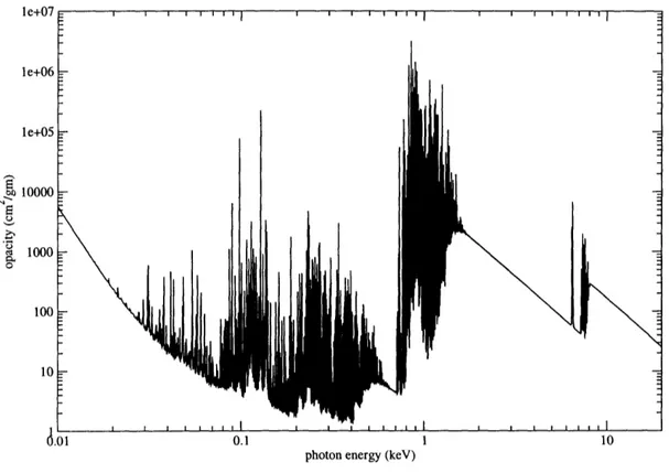
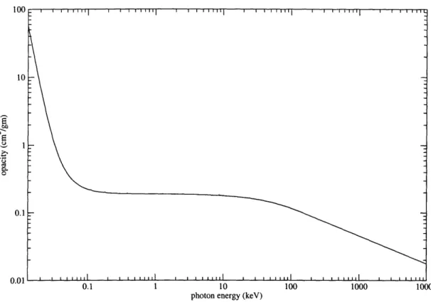
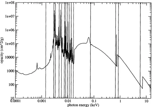
5-1 Iron opacity for T = 0.1 keV and p = 0.0004 g/cm3. The opacities in these plots have been normalized by the material density, hence the change in units from the 1/cm seen previously ... 62 5-2 Iron opacity for T = 5 keV and p = 0.0004 g/cm3 _... _. ₆₄

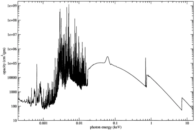
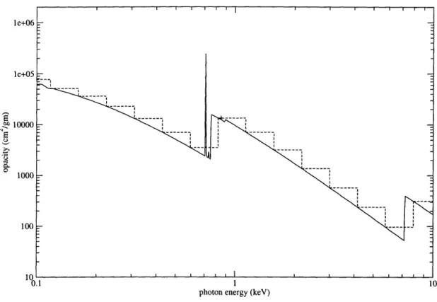
5-3 Iron opacity for T = 0.5 eV and p = 0.0004 g/cm3 ... . 65 6-1 A small section of an opacity plot (solid line) superimposed with a

corresponding set of multigroup opacities (dashed line). Notice that in this example, the group boundaries are uniformly spaced in log-energy space. Notice also that the discontinuous function represented by the multigroup opacities maintains the general character of the original opacity function, but misses smaller features such as the spike just

below lkeV ... 72 6-2 An example opacity on which the equal arc length projection method

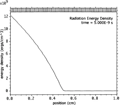
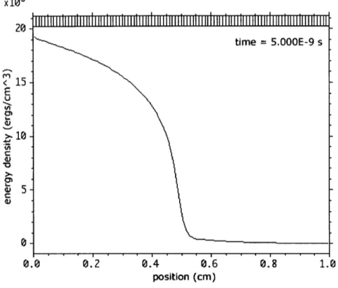
has been performed. The vertical lines indicate the group boundary selections made by the algorithm. Notice that the region of dense bound-bound transition lines has very high group resolution while the relatively smooth regions are characterized by broad energy groups. 76 9-1 The radiation energy density as a function of position. In this example,

the driving wall temperature is 100 eV. ... 108

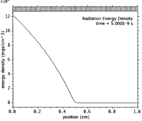
9-2 The integrated radiation energy density as a function of position for multigroup transport. In this example, the driving wall temperature

(12)

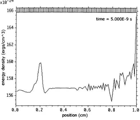
9-3 The multigroup radiation energy density in group 9, spanning photon energies from 100 keV to 316.2 keV. Note the exponent on the ordinate values-this is at the limit of machine precision and consists entirely

of round-off artifacts. . . . ... 110

9-4 The multigroup radiation energy density in group 1, spanning photon

energies from 0.1 eV to 31.62 eV. ... 111

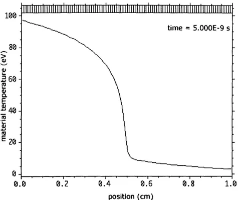
9-5 The material temperature at the time when the integrated radiation

energy density propagation front reaches 0.5 cm. ... 112 9-6 The frequency-integrated radiation energy density for a Marshak wave

with a 500 eV driving wall temperature, showing the difference in out-put for grey and 10-group multigroup diffusion simulations. The time required for the grey solution to propagate half-way through the slab,

as shown in this plot, was 2.4 x 10-11 s. ... 113

9-7 The multigroup radiation energy densities for a 10-group Marshak wave with a 500 eV driving wall temperature, showing each group's

contri-bution to the integrated total. The numbers in parenthesis next to each

group label are the group boundaries for that group. All ten groups are plotted on the same scale; those not listed in the legend contributed

too little to appear ... 115

9-8 The Planck spectrum for a 500 eV wall temperature. The vertical lines are the group boundaries used in the initial 500 eV Marshak wave simulation. ... 116 9-9 The frequency-integrated radiation energy density for two ten-group

simulations with different high-energy limits. The solid line data has a high energy limit of 1000 keV. The dashed line has a high energy limit of 30 keV. Both high energy limits are in a region of energy space which contains negligible photon populations. ... 118

(13)

9-10 The frequency-integrated radiation energy density for two ten-group simulations with different energy limits is compared to a high-resolution 1000-group simulation. The solid line data is the 10-group run with an energy limit of 70 keV. The dashed line is the 10-group run with an energy limit of 30 keV. The dotted line is the 1000-group high resolution data. ... 119 9-11 The opacity for iron at a density of 0.005 g/cm3 _{and two different}

temperatures. These temperatures represent the starting "cold" slab

and the equilibrium temperature of the hot driving wall. The two opacity data sets have different limits as is shown here. The TOPS code extrapolates along a curve of -3 for opacities off the table. .... 121 9-12 The normalized RMS error in radiation energy density as a function of

group count ... 123 9-13 The normalized RMS error in radiation energy density as a function of

group count. Comparison of two different energy limits at small group counts ... 124 9-14 An examination of the falloff in accuracy as the number of coarse

groups is decreased. The number of high-resolution groups and the energy limits are held constant. ... .. 127 9-15 An examination of the improvement in accuracy available by enabling

adaptive multigroup for the 500 eV Marshak wave. These simulations were conducted at the best-case energy limits for the 10-group static

multigroup data. . . . ... 130

9-16 An examination of the improvement in accuracy available by enabling adaptive multigroup for the 500 eV Marshak wave. These simulations were conducted at the worst-case energy limits for the 10-group static

(14)

9-17 Two static multigroup diffusion data sets compared against an adaptive multigroup diffusion data set. The best accuracy points on both static plots still have higher error than the corresponding adaptive multigroup

(15)

Chapter 1 Introduction

Accurate radiation1 transport simulations play a crucial role in high energy density physics. This includes areas of research such as astrophysics[36] and laser physics

as well as emerging technologies like inertial confinement fusion[2, 18, 19]. In each

of these examples, the material energy density is strongly coupled to the radiation field. In fact, the interaction between radiation and the material is so strong that the

radiation tends to drive the hydrodynamics.

In order to understand the dynamics of such a high energy system, an accurate depiction of the radiation transport involved is critical. Furthermore, high energy density physics experiments tend to be prohibitively expensive (or, in the case of astrophysics, impossible). This expense generally leads to very few experimental data points being available and the bulk of the scientific endeavor must be done in simulation.

Unfortunately, radiation transport in current continuum radiation hydrodynamics

simulations is handled in an overly-simplified manner which drastically impairs the predictive capability of many simulations. This is primarily a result of the enormous computational expense of high-accuracy radiation transport methods. While sim-plifying assumptions like the grey diffusion approximation make the computational issues more tractable, they are only valid in certain physical regimes. The multigroup

1_{Throughout this thesis, we adopt the vernacular of the computational physics community at}

Los Alamos National Laboratory, for whom "radiation" refers specifically to photons and does not

(16)

diffusion method, which acts as a compromise between full transport and grey dif-fusion, does not return sufficient improvement in accuracy for low group counts to be worth the added computational cost. This thesis shows, for the first time, that when the number of energy groups is small, traditional static multigroup radiation diffusion's accuracy is not predictable and that unintuitive situations arise in which adding groups can lead to a significant reduction in the accuracy of the simulation.

This thesis develops a unique method for maximizing the accuracy gained from the multigroup radiation diffusion technique and removing the uncertainty in accu-racy caused by a static selection of group boundaries. In simulation environments where the energy group count is limited, the accuracy gained is a function of the correlation between the opacity structure in the problem and the location of the en-ergy group boundaries. If the problem being simulated involves significant changes in the opacity, then the accuracy gained by using multigroup diffusion can only be maintained if the group boundaries shift to accommodate the new opacity structure. The adaptive multigroup radiation diffusion code developed for this thesis is the first implementation of this concept. The static energy group boundaries used by a con-ventional multigroup diffusion package are modified dynamically to suit the current

state of the simulation.

It is shown that this technique delivers improved accuracy when compared to standard multigroup diffusion with static group boundaries. This is equivalent to being able to use fewer groups to maintain a given level of accuracy, and thus re-duces the computational cost of multigroup radiation diffusion. This increases the likelihood of higher-accuracy radiation transport approximations being used in lieu of grey diffusion. The sensitivity of the static multigroup method to group bound-ary placement when the group count is low has made many computational physicists reticent to use the technique despite it's capacity for a more accurate simulation of radiation transport. The introduction of adaption in energy space removes this sen-sitivity and thus provides the user with a predictable increase in accuracy for the increased computational cost of using multigroup diffusion.

(17)

Chapter 2 Properties of the Radiation Field

The interactions of photons and matter can result in significant changes to the local environment of the material. Even in simulations for which the material is considered to be static, the coupling between material and radiation can strongly influence the outcome. However, before we can consider the coupling of radiation and matter, we must first develop a description of the radiation field itself.

2.1 Photon Number Density and Specific Intensity

The radiation field is a complicated entity and is a function of position, time, propa-gation angle, and energy[24]. One way to look at the radiation field is as a collection of photons-each of which, at every instant, has a specific position, direction of prop-agation, and frequency. The quantity used to describe the radiation field in this way is the photon number density, AJ. The photon number density is defined such that the number of photons per unit volume at location x and time t, with frequencies between v and v + dv , propagating at velocity c in direction in into a solid angle dQ is Af(£, t, in, v)dQdv. The units of photon number density are cm-3 sr-l Hz-1[22].

Each of the photons in the radiation field carries with it some energy, E = hv. If we take the photon number density and multiply it by hv, we produce the radiation

energy density, . This is a measure of the energy contained in the radiation field

(18)

frequency v. The relationship between photon number density and radiation energy density is simple but important:

(x, t, n, v) = hviA(, t, n, v) (2.1)

If we take the radiation energy density and multiply it by the speed of light, c, we produce a quantity called the specific intensity, I.

I(x, t, n, v) = c£(, t, n, v) (2.2)

The specific intensity is a measure of the transport of energy within the radiation field. It is defined such that the amount of energy transported by photons of frequencies between v and v + dv through a surface element dS into a solid angle dQ in a time interval dt is

dE = I(, t, in, v)dScosOdQdvdt (2.3)

where 0 is the angle between the propagation vector, ii, and the normal to the surface element, dS [22]. Specific intensity has units of ergs s- 1cm- 2 Hz-1 sr-l. As defined, the specific intensity gives a complete instantaneous description of the radiation field'. It is useful to examine various angular averages or moments of specific intensity which have physical significance.

2.2 Radiation Energy Density

Rearranging equation 2.2 gives us the following formula for the radiation energy density

£(, t, ii v) = I(, t, , v) (2.4)

1This is not absolutely true as we have clearly ignored polarization in this definition. However, polarization is generally not considered in most aspects of computational radiation transport as its effects on radiation/matter coupling are usually negligible.

(19)

If we integrate this over all solid angles, we get

6(x, t, ) =

!

J I(Y, t, , v)dQ

(2.5)

This is referred to as the monochromatic radiation energy density because it is still a function of photon frequency though the angular dependence is gone. It has units of ergs cm-3 Hz- 1. To get the total radiation energy density, we integrate over all frequencies to get

£(Yt)

=

-jJI

(,t, ni,v)dQdv

(2.6)

Total radiation energy density has units of ergs cm- 3 [22].

2.3 Radiative Energy Flux

The first-order moment of the specific intensity-the specific intensity multiplied by propagation angle and then integrated over all solid angle-is referred to as the monochromatic radiation flux

F(i, t, v) =

f

I(, t, ii,

v)idQ

(2.7)

and has dimensions of ergs s-1 cm- 2 Hz-1 [24].

To understand what the flux means physically, consider that the total number of photons crossing a differential surface element dS per frequency interval and unit time, and from all solid angles, is just the photon flux, Acin, integrated over all solid angles and dotted with the surface element

N = (J (, t,

)dS

,

v)cdQ)

(2.8)

This equation can be multiplied by the energy per photon, h, to instead give a value for the total energy crossing dS.

(20)

Recalling the relationship between the specific intensity and the particle number density (equations 2.1 and 2.2), we can show that equation 2.9 is equivalent to the definition of monochromatic radiation flux given in equation 2.7 dotted into the dif-ferential surface dS. Therefore, we can say that the monochromatic radiation flux,

F(, t, v), is defined such that F. dS gives the net rate of radiant energy flow through dS per unit time due to photons with frequency v.

Another quantity of interest is the integrated radiation flux which is simply the monochromatic radiation flux integrated over all frequencies

F(, t)-;

F( , t, v)dv

(2.10)

and has dimensions of ergs s-1 cm-2. In English, the integrated radiation flux dotted into a differential surface dS is defined as the net rate of total radiant energy flow

through dS.

2.4 Radiation Pressure Tensor

Taking the second-order moment of the specific intensity gives the radiation pressure tensor

P(Y, t, v) =

I(,

t, , v)iinidQ (2.11) c

the components of which have dimensions of dynes seconds cm- 2 [22]. The physical meaning of this quantity is best revealed by first examining photon momentum. If a photon has energy hv, its momentum is hni. If we multiply the photon number density by the momentum per photon we get a monochromatic radiation momentum

density vector which, via equations 2.1 and 2.2, is equal to

hv

P

-hfi(x, t, , v)

:

(2.12)

1 (2.13)

(21)

Comparing equation 2.13 with equation 2.11 reveals an interesting similarity. Com-bining the two gives

P(x, t, v) = /

cidQ

(2.14)

The quantity c is the photon velocity vector, so the physical meaning of the radi-ation pressure tensor is simply a means of describing the advection of momentum density. The specifics of what component of the momentum density is being advected in which direction is easily seen when we look at the radiation pressure tensor in

com-ponent form, replacing the specific intensity with the photon number distribution via

equations 2.1 and 2.2:

Pij(, t, v) =/(A(Y, t, , v)cni)(-nj)dQ

(2.15)

The above equation can be interpreted as the net flux of radiation momentum in the

j direction per unit time due to photons at frequency v through a unit area oriented

perpendicular to the i direction. As it turns out, this is exactly the definition of

pressure in a fluid which is why this quantity is referred to as the radiation pressure [22].

When the radiation field is isotropic, the radiation pressure tensor becomes di-agonal and isotropic. In this case, it can be reduced to the average of the didi-agonal components of P, a scalar "hydrostatic" pressure which is referred to as the mean radiation pressure

1

P -(PI + PVy

+ Pz)

(2.16)

3

Combining this with equation 2.11 gives the full form of the mean radiation pressure

P(, t, v) = 3

I , t,

n, v)dw

(2.17)

And this, in turn, can be combined with equation 2.2 to reveal

(22)

which is to say that the mean radiation pressure is one third of the monochromatic radiation energy density when the radiation field is isotropic [24].

(23)

Chapter 3 The Equation of Radiation

Transfer

Now that we have developed a thorough description of the radiation field and some of the quantities derived from it, we can proceed to examining how the radiation field changes in time. The principal mechanisms for altering the radiation field are

photon advection and interaction with the matter through which the photons are

advecting. In the absence of matter interaction, photons move in straight lines at a constant speed of c. Their advection and its effects on the specific intensity can be described in purely mechanical terms and this will not be covered here. Rather, we will concentrate on the much more complicated photon-matter interactions.

3.1 Absorption, Scattering, and Total Opacities

As photons travel through matter, some number of them will be absorbed by the material and their energy will be lost from the radiation field. This loss of photon number density and energy density from the radiation field is described by a quantity called the absorption opacity, a (Y, t, ni, v). The absorption opacity is defined such

that a beam of photons having specific intensity I(, t, ii, v) moving through a piece of matter with differential cross section dS and thickness dl for a time interval dt will

(24)

lose an amount of energy given by

dEa = a(x, t, , v)I(X, t, n, v)dldSdQdvdt (3.1)

The absorption opacity is the product of an atomic absorption cross section (with units of cm2) and the number density of absorbing atoms (with units of cm-3) summed over all atomic states that can readily absorb photons of frequency v. The units of

Ka are therefore cm-l [24].

The other process that serves to remove energy from a beam of photons is scat-tering. Although scattering doesn't remove photons from the radiation field (the integral of Af over all angles and frequencies remains the same), it does change the propagation angle and possibly the frequency of the scattered photon and therefore redistributes the photon elsewhere in phase space. As with absorption, scattering serves to remove energy from a beam of coherent photons. There is a corresponding

scattering opacity,

(Y,

t, in, v), which is defined in the same way as Ka except that the events leading to beam energy loss are scatters instead of absorption [24].

The absorption opacity and scattering opacity can be combined linearly to form what is called the total opacity, jt(:, t, v), because it is assumed that absorption and

scattering events occur independently of each other.

Kt(x, t, ) -

Ka(,

t, ) + Ks(X,

t, )

(3.2)

The total opacity describes the tendency of a beam of photons to lose energy due to

interactions with matter. The assumption is that scattering and absorption are the

only two events that will cause a beam of photons to lose energy. The amount of energy lost can be written as

dE =

K

t(, t,, v)I(x, t, , v)dldSdQdvdt

= [Ka(s, t, in, v) + K,(, t, in, v)]I(, t, i, v)dldSdQdvdt (3.3)

(25)

photon can travel before undergoing either a scattering event or being absorbed into the material and is referred to as the photon mean-free-path, A.

1

AX(, t, n, v) = t (3.4)

rtt, t, V)

It is particularly important to this thesis to point out that the frequency

varia-tion of the above defined opacities can be exceedingly complicated. The structure of the opacity vs. frequency spectrum is a result of contributions from virtually count-less atomic transitions (bound-bound, bound-free, and free-free) and the changes in atomic interaction cross section that occur over each transition.

3.2 Emission

The remaining major interaction event between photons and matter is the emission of photons by atoms. As a beam of photons travels through a medium, some atomic emissions could have an appropriate propagation angle, frequency, position, and time such that they effectively add to the specific intensity of the beam. This phenomenon is described by a quantity called the emissivity, q7(x, t, i, v).

The emissivity is defined such that the amount of radiant energy released by a material element of cross section dS and length dl into solid angle dQ around direction

n with frequencies between v and v + dv in a time interval dt is

dE, = r/(Y, t,

in,

v)dldSdQdvdt (3.5)

Emissivity has units of ergs cm- 3 sr- 1. It is calculated by summing the products of atomic state populations and transition probabilities over all processes that can result in the emission of a photon at frequency v [22].

It is important to understand that photons entering a particular point in phase space (, t, ni, v) via thermal emission from atoms are indistinguishable from photons entering the same point in phase space as a result of a scattering event. Therefore, we break the total emissivity (t from here on) up into two components-the thermal

(26)

emissivity, 7T, and the scattering emissivity, qr. The thermal and scattering

compo-nents of total emissivity are independent of each other and can be added linearly.

3.3 The Transfer Equation

At this point we understand the radiation field and the various material-photon

interactions that can alter it. The next step is to derive an equation which describes the time dynamics of the radiation field and incorporates all of the processes described above. This equation is called the radiation transfer equation.

Consider an element of material with differential cross section dS and thickness

dl. In a time interval dt, we are interested in the change in the specific intensity of

a beam of photons with frequencies between v and v + dv, traveling into solid angle

dQ along a direction in normal to dS. The difference in the specific intensity between (5, t) and (+ AS, t + At) must be a result of energy lost to scattering and absorption

and energy gained through emission. This can be written as

[I(Y +

A,

t +

At, ii,

v)

-

I(, t, n, v)]dSdQdvdt

=

[t(y, t, i, v) -

t(, t, ii, v)I(x, t,

n,

v)]dldSdQdvdt

(3.6)

and simplified to the standard form of the radiation transfer equation

)I(

)

=

).

(3.7)

The left-hand side of this equation is what is sometimes referred to as the "convective" derivative of specific intensity. A convective derivative is a derivative taken with respect to a moving coordinate system, also called the Lagrangian derivative. It takes into account all changes in specific intensity as a result of local sources and sinks of photons, as well as contributions from photons moving in and out of the local area. Separating the left-hand side of this equation allows us to write the transfer

(27)

equation as a conservation equation:

-I(° , t, n,

v)

= ct(,

t,

n, v)-

ct(,

t, n,

v)I(,

t,

n, v)

at

-c(n. V )I(z, t, n, v)

(3.8)

In this form, the physical meaning of the transfer equation is obvious. The change in time of specific intensity is equal to the photon sources minus the photons sinks. In this case, the sources of photons are given by the total emissivity plus the photons that enter position Z due to advection, while the photon sinks are comprised of the total opacity times the specific intensity and the photons that leave position x due

to advection.

3.4 Moments of the Transfer Equation

Just as the moments of the specific intensity revealed useful physical quantities, so will moments of the transfer equation. To obtain the zeroth order moment equation,

we integrate equation 3.7 over all angles

1_at_I(

_{t, ,}

_v)dQ

₊

_J(ii

_V-)I(,

_{t, i,}

_{v)dQ =}

[h(X,

t, ,

v)

- t(Y, t,

,

)I(Y, t, , uv)]dQ

(3.9)

The first term can be written as a function of the radiation energy density by combin-ing it with equation 2.5. Similarly, the second term can be combined with equation 2.7 to be written in terms of the monochromatic radiation flux. These two manipulations produce the following form of the zeroth order moment equation:

at

(

_,

_t,

_{) +}

_{V. F(x,}

_{t, )}

_{= [/(}

_{t ,}

_{) -}

_t(,

_{t, n,}

_)I(,

_t,

_n,

_{v)]dQ (3.10)}

In this form, the zeroth order moment equation is a conservation equation for radiation energy density. The terms are easily described physically. The time rate of change in monochromatic radiation energy density at frequency v is equal to the sum of all

(28)

energy emitted at frequency v by the material, minus the sum of all energy in photons of frequency v absorbed or scattered by the material, minus the net flow of energy in photons of frequency v through the surface containing the volume element (the V F term).

The first-order moment equation for the radiation field is obtained by multiplying the transfer equation (3.7) by i and integrating over all angles. By incorporating equations 2.7 and 2.11, this treatment produces the following form of the first-order moment equation

1a 1

2 F(Y t V)1 + P(, t v) =-

J[,qt(Z

t n v) - t(Y, t, n, v)I (x, t, n, v)]ndQ (3.11)

C2at C

Substituting equations 2.7 and 2.13 into the first term of equation 3.11 reveals that this is just the time derivative of the radiation momentum density integrated over all propagation angles. Recall also from equation 2.15 that P is the radiation momentum flux density tensor. Clearly, then, the first moment of the radiation transfer equation is effectively a conservation equation for the radiation momentum density and is analogous to the hydrodynamical equations of motion.

The physical interpretation of equation 3.11 is that the time rate of change of monochromatic radiation momentum density for photons at frequency v is equal to the negative of the volumetric force exerted by radiation stresses caused by photons at frequency v plus the net momentum gained by the photons of frequency v in the radiation field from interactions with the material.

3.5 Local Thermal Equilibrium

The radiation transfer equation and its moments are reasonably complicated and are difficult to solve in any sort of general sense. There exist, however, certain cases for which the transfer equation is greatly simplified. Local thermal equilibrium (LTE) is

one such case.

(29)

adiabatic system is said to be in strict TE if it is in steady-state equilibrium and contains a homogeneous material. In this case, the material must have the same temperature everywhere--otherwise temperature gradients would exist, inducing heat flow and the loss of steady-state. For the same reason, it is safe to assume that the radiation field is isotropic and homogeneous. Furthermore, because the material is exhibiting blackbody radiation (and thereby losing energy), the rate of photon absorption by the material must be such that the energy gained by the material by said absorption exactly cancels the blackbody radiation. The mathematical version

of this statement is

r7T(V) = ia(v)I (fi, v) (3.12)

and is known as Kirchoff's law.

Material in strict TE at temperature T has specific intensity described by the

Planck function

B(v, T) = 2h (ek - 1)- 1 (3.13)

where k is the Boltzmann constant, 1.3806503 x 10-23 m2 kg s-2 K- 1. Equation 3.13

combined with equation 3.12 leads to the Kirchhoff-Planck relation [22]

?7T(V) = Ka(v)B(v, T) (3.14)

The Kirchhoff-Planck relation only holds true for strict TE. However, if the ther-mal gradients in the material are so sther-mall that the change in temperature over the mean-free-path of a photon were negligible, then we can assume that equation 3.14 will offer a good approximation at the local values for the thermodynamic variables. The reasoning is that a photon will be thermalized by the material long before it sees a significant difference in temperature, so in the region through which the photon streams, the thermodynamic variables are essentially constant and a "local steady-state" can be assumed. This is the fundamental hypothesis of LTE.

(30)

local values of position and time.

T(X,

t, V)

= r'a (Y,

t, )B[, T(, t)]

(3.15)

Furthermore, if we assume that the scattering that takes place in the system is co-herent and isotropic, then we can write the scattering emissivity as

Us=

4f-JIdQ

(3.16)

and therefore the entire emissivity can be written as

r7t

=

ia(X,

t, v)B[v,

T(i, t)]

+

(

)

I(,

n

t,v)dQ

(3.17)

3.6 The Diffusion Limit

In regions of high optical depth and low photon mean-free-path, photons interact fre-quently and have a tendency to undergo many interactions before traveling a distance comparable to the scale lengths of interest. Photons "diffuse" through matter in a random walk of scattering events until they are absorbed. High electron density and high temperature makes for frequent electron scattering events which rapidly drive the electron energy spectrum to equilibrium. Any effect on the material energy by the coupling to the radiation energy field is equilibrated effectively instantaneously. This environment supports a condition of LTE [23].

The principal assumption of the diffusion approximation is that the photon mean free path is much shorter than the scale lengths of the problem, i.e. A <K 1. In the limit

that this is true, a perturbation analysis of the radiation transfer equation provides a

rigorous and elegant derivation of the diffusion limit of transport. To begin, we start with the transfer equation (3.7) and rewrite it in the following form

a(BI)S(I)

(3.18)1

(31)

where S(I) is the scattering operator allowing for photon scattering in angle and frequency. Here we have made the assumption of LTE, which dictates that the thermal emission spectrum is always Planckian and the thermal emissivity can therefore be written as KaB(Tm) where Tm is the material temperature. The LTE assumption also simplifies the scattering operator as will be seen shortly. Unlike strict TE, however,

LTE allows for the material and photon temperatures to differ. In the limit that A/l

is small, the material and radiation temperatures will be similar. We will assume for

the purposes of this derivation that the matter temperature, T,, and the radiation

temperature, Tr, are similar such that the energy exchange between the radiation field and matter is slow enough to compete with transport, i.e. (Tm - Tr)/Tr < 1.

In the diffusion limit of small A/l, we can say that Tm- Tr is also small. Writing

equation 3.18 as

I I

at +

(. V)I =

i(B(T,)

-

I

+

B(Tm) - B(Tr)) - S(I).

(3.19)

c Ot

we can treat B(Tm) - B(Tr) as small. This is the matter-radiation energy exchange

term.

The Scattering Operator

We now turn to consider the properties of the scattering operator, S, on the specific

intensity, I. We start from the form of the operator (for Compton scattering of photons off free electrons) used by Sampson[39]. We express the operator in terms of

the photon distribution function to help elucidate the physics and to simplify proof

of the operator's conservation law properties. Sampson's formulation for S(I) is

S(I)

=

N(pTm)dp(v

-

v',Q Q')I(v,

)[1

+

,3

I

(V',')]-dv(p'

I(v',)[1

)

(P

,

Tm)dPp'c

(V' --

vQ'

-+

s(v,

+-a

Q)] dQ'

(3.20)

(32)

scattering from initial frequency v to final frequency v' and from initial propagation angle Q to final angle Q'. N(pe, Tm) is the number density of electrons with momentum

Pe-We will rewrite this using the following definition

I = hvp(v)n,

(3.21)

where n, is the distribution function for photons at frequency v and p(v) is the density of states for photons with frequency v

2v2

p(V)-

2 .

(3.22)

Rewriting the scattering operator as a function of n, leads to

S(n _,) = ( N(pe, Tm)dpeo(v O v', Q - Q') 2 n(1 + n,_,)

-J

N(P',Tm)dp

LT(V'

-9

vdQ' Q

2

hv n, (1 + n,)}dQ'.

(3.23)

This can be written in a more symmetric form by reintroducing the frequency integral and associated energy conservation delta function

1

X

fo

ddv6(v-

Ee-

Ee

)

(3.24)

along with the principle of detailed balance, which tells us that the probability of transition from (v, Q) to (v', Q') is equal to the probability of the inverse process. Sampson writes the principle of detailed balance like this

U(v -+ v', Q + Q')V2_ddpe _{= (VI'}_- _{vQ,-'_ Q) v'}2_dv'dp'e. _(3.25)

If we define the following shorthand for the transition rates

(33)

,

= -' v, Q' - Q)dpecp(v') (3.27)

(3.28)

we can express the scattering operator as

S(n,)

=

dQ'

dv'

dpe

C2

XhVTvviN(pe, Tm)nv(l + n',)6(v

_{-2 jdQ'}

_dv'fj

dp'

-

v/'

-(EeE))

xhvf,vN(p'e, Tm)n

,(1

+ n)6(v - ' - (Ee - Ee)) (3.29)

These two terms represent the amount of energy lost and gained by the intensity, I = hvpn,, as the result of scattering.

We can split up the energy conservation delta function into a portion which assumes fully elastic Thompson scattering and a term which accounts for inelastic Compton energy exchange by incorporating this equality:

6(v

-

'

- h(Ee

-

E))

= 6(-v') +

[6

- v

-h(E

-E )) -

(v

- v') (3.30)

where we assume that 6(v-v') is leading order while [(v - v'- 1(E - Ee)) - (v - v')

is a second order contribution. Substituting this equality into equation 3.29 allows us to write the following

S(n,) = selastic(n) + SCompton(n) (3.31) where Selastic (n) = 2 jdQ' dv' dp x

hvT,,,vN(pe,, T.)n (l + n,)6(v

v')

-2 j dQ' dv'j dp x c2hv N T) + (3.32)

h'T,,vN(p'

, Tn)n,,

( + n,)( - v') .

(3.32)

(34)

and

sCompton

v

4

_C2_r

dQj

_/ _t°

dv'

dphvT÷vN(p4, Tm)nv(l + n,) x

(v-,

-

(Ee

- E'))

-2 -dQJ d dpehvTlN(pe, Tm)n,/(l + nv,) x

6(v - ' -(Ee - E))- s"elatic(n,) (3.33)

The energy conservation properties of Selastic(nv) can be shown by integrating over all angles and photon frequencies.

dQ

j

°

dvSelastic

(n ) -

c

dQ

jf

d'v dQ'

j

dv' dpe x

hvTv-v.N(pe,*

Tm)nv(l + nv)6(v v')

-2

jdQ

dQ

dQ'fo

d

/f

dp'e

hvT,,.N(p'e, Tm)n'(1 + nv)6(v - '). (3.34)

By swapping which frequency we denote with the prime in the second term, we can show that the two terms are equal and cancel each other. The result is, as expected, that the total change in energy due to Thomson scattering is zero. In equation 3.30, we assumed that the elastic scattering component was leading order while the Compton contribution was a second-order correction. This indicates that the complete scattering operator conserves energy to first order. We can write this in terms of specific intensity

/dQ do°dSelastic(I)

=

0.

(3.35)

The fact that scattering conserves energy to first order for any specific intensity is significant and will play an important role in the perturbation analysis, below.

The scattering operator drives the radiation intensity to the blackbody distribu-tion at the matter temperature. In equilibrium, with no transport, the absorpdistribu-tion

(35)

material. In order to maintain a steady state, the in-scatter and out-scatter from

any point in specific intensity phase space must also exactly cancel. This mandates a fully-balanced scattering operator and we can say that S(I) = 0. The balanced nature of the scattering operator in equilibrium allows us to reduce equation 3.29 to

N(pe, Tm)n,v,(

+ n,') = N(

1

p, T,)n,

(l1

+ n,).

(3.36)

If we now define a substitution variable

n,

1 + n (3.37) we can rewrite equation 3.36 as

^, ,

N (p-,

Tm)

Tnou N(Pe, Tm) fl, N(j3~e,T)

The factor on the right hand side allows us to write

(3.38)

is described by the Saha-Boltzmann equation, which

n' exp(- hV

n

kT., (3.39) n,, exp(-_ k,1

-Separating the variables here shows that

=

(hv

TE = exp(-k

)

mT,

and therefore, via equation 3.37,

1

nv =

Substituting this and equation 3.22 into equation 3.21 shows that

2hv3 1

c2 exp( kT )-

1

Comparing this equation to 3.13 shows that this is the definition of the Planck

dis-(3.40)

(3.41)

(36)

tribution. Starting with the statement that we are in equilibrium, we are able to

conclude that I = B and furthermore that S(I) = O. Therefore, we can say that

S(B) = 0. (3.43)

Perfect balance of the scattering operator is only true when in equilibrium, so we can

also say that if S(I) = 0 then I must be B.

In equation 3.19 we split the temperatures such that we could account for the possible difference between Tm and Tr. The result is a difference term, which is assumed to be small, and a dominant Tr term. In order to write the complete transfer equation with the same dominate temperature, we must also split the electron number density term in the scattering operator in the same way

N(pe, Tm) = N(ie, Tr) + N(Ye, T.) - N(/e, T,). (3.44)

where we can treat N(/ei, T) - N(pe, TR) as small.

Perturbation Analysis

Now we take the rewritten transfer equation and expand the specific intensity in powers of e = A/l:

I = I0 + I

1

+ I2 + ...

(3.45)

In this way, we expand about thermal equilibrium and ensure that all of the frequency-and angle-integrated specific intensity is contained in Io. To construct an ordering for the operators in the radiation transfer equation, we start with the collision term, which goes as 1/A, and assign it an order of 1. In order to make it dimensionless, we must multiply by a factor of A. The advection term goes as 1/1, so when multiplied by A it goes as A/l = . We assign the (B(Tm) - B(Tr)) term in the energy exchange operator to be order 2 on account of the assumption that (T - T)/Tr < 1. The

time derivative term is assigned an order of E2_{because this is the only ordering which}

(37)

out the order of each operator in the transfer equation C = 0 (1) (3.46) (n. V) = 0(c) (3.47) = (62)

(3.48)

c Ot X = O(E2) (3.49)

where we have used the C notation to denote the non-linear collision operator which

includes both absorption and scattering terms

C(I) = (B(T) - I) - S(I)

(3.50)

and the X notation to denote the exchange term, which handles the effects on ab-sorption due to a difference between material and photon temperatures

X = Ka(B(Tm) - B(Tr)). (3.51)

All of these operators are linear in specific intensity except for the collision op-erator. As a result, simply applying the collision operator on 2 does not produce the full second-order collision terms. There are nonlinear terms in I1 as well as Io terms combined with a second-order representation of electron number density or the second-order Compton energy delta function. In order to perform a proper perturba-tion analysis, we must first expand C(I) and collect terms by order.

To begin, we substitute equation 3.45 into equation 3.50 to obtain

C(Io + I1 + 2) = KI(B(T) - Io - I1 - 2) - S(IO0 + I1 + I2) (3.52)

The non-scattering terms can be ordered immediately:

KiaB(Tr) =

(1)

(3.53)

(38)

IaI = O(E) (3.55)

1aI2 = (c2)

(3.56)

Next, we expand the scattering term S(Io + I1 + 12) and order the results. To do

so, we need to take into account the temperature splitting in the electron number density, as described by equation 3.44, and the splitting of the elastic and inelastic scattering contributions described by equation 3.30. We assert that the quantity

(T, - TR) is (e2). Therefore, we can treat the term N(pe,T,) as 0(1) and the

quantity (N(p, T) - N(pe,Tr)) as (e2). The elastic delta function b(v - v') is

treated as 0(1) while the Compton delta function,

6(v

- v' - (E - E')/h) -

5(v

- v') is treated as O(e2). These orderings will allow all of the energy exchange terms to compete at second order.

We are only keeping terms up to second order, so the scattering terms that include the second-order electron number density only need to have the zeroth-order specific intensity included. As this expansion is relatively simple, we'll handle it first. Sepa-rating the scattering operator on the two halves of the second-order electron number density gives us

S

2

nex(I) =

-

f

O

dv'

jN(pe,Tm)dpe(v -

u',Q

-+

Q') x

C2 o[i + 2-h ,3(16( _2hv'3 - ') - _'

dv'

AN(PN,

Tm)d

(v'

V,Q'

--

Q)

--

x

fo fo e e V/ d C2

IO[1

+ 2h

30 o](

-

')

-j

dv' j N(pe, T,)dPeO(V i', Q Q') x

C2

Io[1

+ 2h ,3I](V - ') +

dv' N(P, eTr)dP'e-(' - ,Q Q)V' d-+ X

I[1 + 2h 3zo](v - ') dQ' (3.57)

(39)

Io(v', Q'). The notation S"ne(Io) indicates that this is a second-order term which is

a non-linear function of Io and arrises as a result of the energy exchange temperature splitting in the electron number density. The terms in S2ne(Io) all contain the elastic

scattering delta function, and are thus part of the Thomson scattering contribution to

total scattering at second order. Physically, S2eneX(Io) is just a second-order correction term which arises as a result of our choice to use N(pe, T,) to leading order rather

than N(p, T).

In a similar fashion, the scattering terms that include the second-order Compton energy exchange delta function only need the zeroth-order specific intensity included.

=

dv

N(pe, Tr)deo(v -+

v',Q

-

Q') x

C2

Io[1 + _2hv'3

I]6(v

- v' - (E -

Ee)/h)

-dv

j

N(p, T)dPe(u'

-+

vv,Q' -+

)

d x

C2

Io[1

+ 2hlo]6(v

-

v

-

(Ee

-

E)/h)

-2hiA

dv

j

N(pe, T,)dPe(V -+

v',

Q -

Q')

x C2 Io1 + 2h 3I](>- v')-dv N(p, Tr)dp'e v(Q' Q-)

-

x 0o% + 2.Co I 1011

±

Io3(v

-

v') }df'

(3.58)

We can now write the total second-order expansion of the scattering operator as the linear combination of terms:

S(

0

+ 1 +

1 2

)

=

So(Io)

+ S (I1) + sin(I

2

) + l(1) + 2Comptn(I

0

) + Senex(Io).

(3.59)

where the subscripts on each term indicate its order, S2in(I2) indicates a second order term that is linear in 2, and S(I ₁) indicates a second order term that is non-linear

in I. The terms which have not yet been explicitly defined can be by doing the full expansion and separating the terms:

(40)

= i dv

JO

N(Pe, Tr)dpeU(v C2 loll + 2h I]( - ')

-dvf

_{N(p', Tr)dpe'('}

-2h3 } = o

J

N(Pe, Tr)dPeu(v

2h'

3 _[Il

_{Io + l Io]j(v}

_')

-dv

j

N(p',

Tr)dpe ,(v' -+ C2

2hV

3_[IlIo

₊

v,Q' - Q) d x v' dv (3.60)

-

v',

Q -- Q')I1 +

V dv'I v' dv IIo](v - vi) }dQ' _(3.61)

'(pe, Tr)dpeo(v -- v', - Q')I2 +

]6( - )

-dvi

_{J N(p, T)dp'(v'}

--[2hv3[2Io + I2Io(v -

v')

IdQ'

r 0 o ro0 = i f dv jf N(pe, Tr)dpea(v C2 I2hvI3B 1

₁

1

_1(v

_- _v) -J

dv

_dy

j

_{N (p',,}

N(P Tr)dP(

_{T ) dp'a (V -+}

fo O e Lr~ ee v dv'

. f4 v' dv

) +

(3.62) --+ v', Q -+ Q') x v, Q' - Q) x So(Io) S1(I1)

=

f

_dvJ[.

C2 2hv'3 [I2Io + I2Io

S (

2

)

S ( 1) -- VI, -+ Q') x

(41)

v dv' c2h

V' dv 2hv3 1 ' )d' (3.63)

Notice that So(lo) is identical to the second half of S2ne(Io) so we can simplify equation 3.57 to

Senex (I0 ) =

So(Io) also appears as 3.58 to 2Comptn(IO)

f

4 dv N(pe, Tm)dpa(u - v, Q -+ Q') x C2 1 + 2hv'3 _] jdv N(p'

Tm)dp'

c(v

- v, Q' - Q) x i'd l+ 2h 3 o ]_-So(Io)}dQ (3.64)

the second half of S°omPt°n(Io), so we can simplify equation0

=

JdvJO

N(Pe.d Tr)dpeo-(v -+

vQ

Q') x

C2

Io[l

+ ]3](- V' - (E -

Ee)/h)-2hv'3

dv

N(,

T)dp-

c(v' - v,Q'

- Q)

v

dv'

I1 + _2hV3+

2hv

3

Io]6(v

-v' -(Ee -Ee)/h)

-

So(Io)}dQ'

(3.65)

Now that we have expanded the scattering operator and ordered the terms, we can assemble the full transfer equation by order and examine the results.

Zeroth Order

If we take only the zeroth-order terms in the transfer equation we are left with

=

ia(B(T)

- Io)

-

S(o).

(3.66)

As we are expanding about thermal equilibrium, we expect the zeroth-order be-havior of the radiation field to be similar to that of strict thermal equilibrium. In strict TE, scattering is fully balanced and thus we expect So(Io) to be zero. If this

(42)

is the case, then the above equation reduces to B(Tr) = o. Substituting this result

back into equation 3.66 leaves us with So(B(T,)) = 0. This expression was already proven to be true in equation 3.43, leaving us with a fully self-consistent result. It is also consistent with the assertion that the zeroth-order behavior of the transfer equation in the diffusion limit is equivalent to strict TE, where the specific intensity is always represented by a Planckian. The zeroth-order expansion of the transfer equation therefore tells us that

Io(i, t, v) = B(v, Tr). (3.67)

Now that we have demonstrated that So(Io) = 0, we can further simplify S2ne(Io) in equation 3.64 to

/o00 00

Senex(Io) = dv'

j

N(pe, Tm)dpeT(v -+ ', -

Q')

x

C2

Io[ + 2h-,I4

i (-

V)-dv'j N(p, Tm)d'ci(v' - v,Q' -+

Q)

x

o

dv I[1

+ 2h3Io]6(v - ') d. (3.68)

which is the same as So(Io) except that the electron number densities are given

at the material temperature while the specific intensities are given at the radiation

temperature. Similarly, we can simplify S2ComPton(Io), equation 3.65, to

S2C°mPt°n(Io)=

J{a

dv' N(pe, Tr)dpe( ', Q Q') X c2

Io[1

+ -2

h

3

IO

(v - - (E, - E)lh)

-dv'

N

(p',

Tr)

dp'(

v'

, Q'

) x

' (E )/) (3.69) d I[1 + 2 lo]6( - '- (E-E)h)dQ

(3.69)

Adaptive multigroup radiation diffusion