Acoustic Logging In Randomly Stratified Formations

FORMATIONS

by

X.M. Tang

New England Research, Inc. 76 Olcott Drive

White River Junction, VT 05001 and

N.Y. Cheng, C.H. Cheng, and M.N. Toksoz Earth Resources Laboratory

Department of Earth, Atmospheric, and Planetary Sciences Massachusetts Institute of Technology

Cambridge, MA 02139

ABSTRACT

The propagation of borehole acoustic waves in the presence of various types of hetero-geneous formations is investigated by modeling them as stratified media with varying velocity-depth distributions. Two types of formations are modeled, using translational and cyclic random models, respectively. Borehole acoustic wavefields for the hetero-geneity formation models are simulated using finite-difference techniques. The wavefield modeling results show that the borehole acoustic waves can be significantly affected by the formation heterogeneities. Specifically, the scattering due to heterogeneity can cause significant amplitude attenuation and travel time delay for the transmitted waves. The borehole guided waves are also sensitive to the formation heterogeneity. The effects of the random formation heterogeneity on the borehole acoustic waves are controlled by two factors: the degree of heterogeneity variation and the heterogeneity scale length relative to the wavelength.

INTRODUCTION

A geological formation is usually heterogeneous. The elastic properties of the formation can vary along the propagation path of the acoustic logging waves. A very good example of the formation heterogeneity is the vertical layering of the sand-shale sequence com-monly found in sedimentary formations. That the geological formation is heterogeneous

can also be evidenced by the fluctuations on acoustic wave velocity (compressional or shear) logs. Although the acoustic wave propagation in a borehole with a homogeneous formation (Biot, 1952; Cheng and Toksliz, 1981) has been well understood, acoustic wave behavior for a formation with randomly varying properties has not yet been stud-ied. This problem differs from the problem of elastic wave propagation in random media because of the presence of a fluid-filled borehole penetrating the random formation. It is interesting to investigate the effects of formation heterogeneity on the compressional and shear wave arrivals of the borehole acoustic wavetrain. Itis also of special interest to study the effects of formation heterogeneity on the propagation of borehole guided waves. The results of these studies will be useful in interpreting borehole acoustic wave logs measured in heterogeneous formations.

We restrict the study to the one-dimensional case, in which the formation is ap-proximated as a laminated isotropic elastic medium, varying only along the borehole axial direction. This approximation is reasonable because vertical layering is a common feature in sedimentary formations. In this study, we adopt two stochastic process-es to dprocess-escribe the laminations by random media. Thprocess-ese two procprocess-essprocess-es are cyclic and translational layering which have been used to model the two main types of sedimen-tation patterns (O'Doherty and Anstey, 1971; Kerner, 1992). The wave propagation in the fluid-filled borehole with a random formation will be computed with a numerical method using the finite-difference technique.

RANDOM MEDIUM MODELS FOR SEDIMENTARY

FORMATIONS

A typical feature of sedimentary rocks is lamination or stratification of the formation. In thiS section, we model two types of the lamination. In the first type, the variation of acoustic properties of the medium across the layer interface is translational (or contin-uous). In the second type of model, the medium is represented by a periodic repetition of layers with two different rock properties. The property change across the layer inter-face is discontinuous. The occurrence of an interinter-face is specified by a Poisson process. Kerner (1992) has adopted these two models to describe stratified sedimentary rocks. We describe the two models in the following sections.

Translational Model

In this model, the medium fluctuation is described as a stationary stochastic process. The medium velocity (compressional or shear) is defined as the sum of the mean value 11 and the fluctuation

av

with depth

z,

as

v(z) =

v

+

6v(z) . (1) The fluctuation 6v(z) can he generated by two methods; the first is based on filtering uncorrelated white noise (which has a Gaussian distribution) with a given correlation function with correlation length a (Frankel and Clayton, 1986; Kerner, 1992). In the second alternative approach, the fluctuation is represented in the spatial frequency k

domain

ov(k)

=

C(k, a)ei21rp , (2)

wherep is the Gaussian random noise (0:5p :51), C(k,a) is the I-D Fourier transform of the spatial correlation function with correlation length

a.

This approach represents the amplitude of the random field using the spectrum of the auto correlation function; the phase is the uncorrelated Gaussian noise. In this paper we use a von Karman correlation function C(r)

=

Ko(~), where K o is the zero order modified Bessel function, whose Fburier transform is (Frankel and Clayton, 1986)

- 2'1l'a

C(k, a) = (1

+

k2a2)1/2 . (3)

The inverse Fourier transform of Eq. (2) gives the spatial variation6v(z). The standard deviation of6v(z) characterizes the degree of fluctuation arround

v.

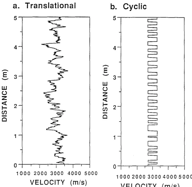
Figure la shows an example of modeling the I-D random velocity variation using Eqs. (1) through (3), The mean value of the velocity

v

=

3000m/s. The standard deviaion of6v is 10% of

v.

The correlation length of the medium is 0.1 m. The velocity shows the gradual variation with depth which is typical for translational layering.

Cyclic

Model

The cyclic (or quasi-periodic) variation can be used to describe the formation which contains mostly two rock constituents (for example sand and shale). The formation velocity varies periodically between the velocities of the two constituents. This quasi-periodic variation can he modeled using the Poisson process (Kerner, 1992).

In the Poisson process p(z), the occurence of an interface between the two con-stituents is controlled by a paremeter

Ii

(analogous to the correlation length in the translational model), which describes the average layer thickness of the layers of various thicknesses. The distribution of the thicknesses is controlled by the Poisson process; p(z) takes on the value of +1 and -1 which are associated with the velocity distribution

( ) _ {VI

p(z)

=

+l

v z - _{V2 P}()

_z

_=-1 , (4)

where the subscripts 1 and 2 denote medium 1 and 2, respectively. The Poisson process has an exponential autocorrelation function, whose correlation length is half of the average layer thickness

Ii

(Jenkens and Watts, 1968). Figure 1b shows an example of modeling a laminar structure by a random medium using the Poisson process. The velocities are

VI

=

3300

mls

and V2

=

2700

mis,

respectively. The average thickness

of the model is 0.1 m. The total model length is 5 m. The cyclic velocity variation in Figure 1b is markedly different from the translational model (Figure 1a).

MODELING BOREHOLE ACOUSTIC WAVE PROPAGATION BY

FINITE DIFFERENCE

In this section, we outline the finite difference method in cylindrical coordinates. We consider a cylindrical fluid-filled borehole embedded in an isotropic but vertically het-erogeneous elastic formation. Assuming azimuthal symmetry (a wavefield independent of the azimuthal angle 0), the elastic wave equation in terms of the radial and vertical components can be written as

Ovr

_~~(rTrr)

_{_ TOO}

₊

_OTrz

(5) p - = fJt _{r or r OZ} Ovz 1

a (

)

OTzz ₍₆₎ p - = _{- f j rTrz}

+ 8

fJt _{r r z}

where _{(vr,vz )} is the displacement vector and (Trr,TOO,Tzz,Trz) is the stress tensor. pis the formation density. The time derivative of the stress strain relation (Hooke's law) is:

8Trr _{..\[10(rVr) Ovz ] 2 Ovr}

(7)

=

- - - + - +

I l

-fJt _{r or oz or}

Oroo

_{..\[10(rVr) Ovz ] 2 Ovr}

(8) fJt

- - - + - +

_{r or oz} I l -_or

8Tzz _{..\ [1o(rvr) OVz] 2 Ovz}

(9) fJt

- - - + - +

_{r or oz} I l -_oz

OTrz _{(OVr OVz)}

(10)

=

Il

+

-fJt _{OZ or}

A

=

p(V_pZ- 2V,Z)

11 pV,z

(11) (12) can be specified by assigning values for velocities

v"

and

va,

and density p. Eq. (5) through (10) are formulated as the first order velocity-stress wave equations. This form of first order equations can be described on a staggered grid with centered finite differ-ences (Virieux, 1986; Kostek, 1991). The advantage of this discretization is that one does not need to treat the fluid-solid boundary explicitly (Virieux, 1986). This provides an easy way to simulate the wave propagation in a fluid-filled borehole surrounded by an elastic formation.

To minimize the size of the computational grid, we choose the rand z axes as symmetry axes. Damping layers are used at the bottom and side boundaries of the grid to absorb the incident waves. The stable condition of this finite difference scheme is given by

(13) where 1::.t is the grid time step, /:;.r and /:;.z are the grid step in r- and z-directions, respectively. Vn=: is the maximum P-wave velocity on the grid. In order to minimize

the grid dispersion the grid size is chosen as

"(A A) Amin

mm

ur,Uz

<

10

(14)

where Amin is the minimum wavelength in the wave propagation problem. The wave excitation is accomplished by applying a point pressure source at the origin. The point source generates monopole acoustic waves in the borehole. By performing the finite difference simulation, waveforms at any distance from the source can be displayed and analyzed.

NUMERICAL SIMULATION RESULTS

In this section, we present results of numerical simulation of acoustic wave propagation in a fluid borehole with various types of stratified formations. In all the examples below, the borehole radius is 0.1 m and the borehole fluid density and velocity are fixed at 1

g/cm

3 _{and 1500}

_mis,

_{respectively. The formation properties are varied to study}

P-wave'Trains

P-wave arrivals are of primary importance because they can be easily identified and processed to determine formation P-wave velocity logs. In order to study the effects of variation of formation P-wave velocity on the P-wave arrivals of the borehole acoustic wavetrain, we vary Vp of the formation using the random medium models described

previously. Although the S-wave velocity and density may also vary as

vP

changes along the borehole, their variations are of secondary effects on the P-wave trains compared to the variation of

v",

especially on the P-wave travel time. We will study the variation of

Va

on P-wavetrain later. Because the P-wave arrivals are most prominent in the form of a leaky-P wavetrain in a slow formation (Le.,

Va

:5VI), we choose to model the wave propagation in a slow formation by setting

Va

=

1300

mls

and

p

=

2.4

g/cm

3_{• The} average formation P-wave velocity Vp

=

2600

m/s.

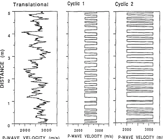
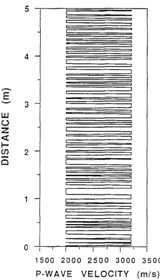
The synthetic waveform logs will

be calculated for three random P-wave velocity models. They are: translational model with 10% deviation and 0.1 m correlation length; cyclic model 1 with

VP,

=

2900

mls

and V_P2

=

2300

mls

and average layer thickness 0.1 m; and cyclic model 2 with

VP,

=

3200

mls

and V_P2

=

2000

mls

and average layer thickness 0.1 m. The velocity variations of these models are illustrated in Figure 2.

For comparison with the random medium results, we generate synthetic borehole acoustic waves for a homogeneous formation with the parameters given above (Le.

Vp

=

2600

mis,

Va

=

1300

mis,

and

p

=

2.4

g/cm

3). The center frequency of the

acoustic source is 10 kHz. Figure 3a shows the synthetics. The leaky-P wavetrain is the most prominent wave in the whole wave train, together with the (weak) Stoneley wave arrivals. Figure 3b shows the synthetic waveforms for a translational model in Figure 2. Comparing Figure 3b with Figure 3a, we see that for this moderate random variation of

v",

the coherence in the moveout of the P-wave train is preserved, but scattered waves appear in the later part of the wave train. The P-wave amplitude is attenuated and the arrival time is slightly delayed compared to the homogeneous formation case. These features are in agreement with the 1-D wave propagation simulation of Stewart et aI. (1984) and Tang and Burns (1992).

Next, we use cyclic model 1 of Figure 2 to calculate the acoustic waveform log. Note that for this model the average P-wave velocity Vp is 2600

m/s.

Figure 3c shows the

simulation results. The waveforms are similar to the translational variation case, except that the scattered waves become stronger. For cyclic model 2 of Figure 2, the fluctuation in

v"

is further increased by setting V_P1

=

3200

mls

and Vp,

=

2000

mls

(note that Vp

is still 2600

ml

s) and keeping other parameters unchanged. The resulting seismograms are shown in Figure 3d. Compared with previous cases, this strong cyclic variation of

v"

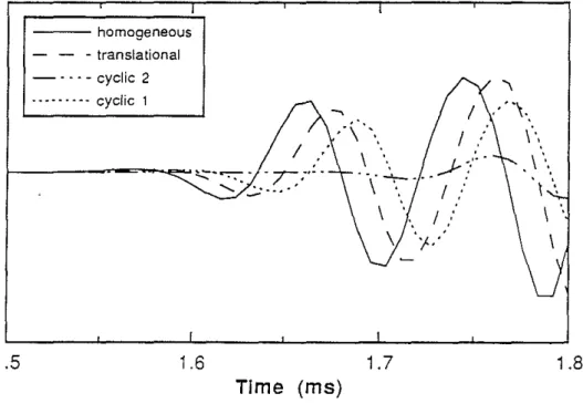
results in strong scattering of the P-wave train, reducing significantly its amplitude and increasing the scattered wave amplitudes. Note that the arrival of the P wave is also significantly delayed. To show this more clearly, Figure 4 plots the waveforms of the first arrival received at 4 m from the source for the homogeneous, translational,

cyclic model 1 and cyclic model 2 cases. The waveforms of the heterogeneous models are attenuated and delayed relative to the homogeneous case. The travel time delays are 0.8% (translational), 1.8% (cyclic 1) and 7% (cyclic 2), respectively. The ampli-tude attenuation and travel time delay of the P-wave train can be used to show that the propagation of these borehole waves also obeys the theory of wave propagation in random media, despite the presence of the borehole.

Tang and Burns (1992) showed that for elastic wave propagation in a random medi-um, the wave attenuation (expressed as l/Q) and velocity dispersion (proportional to the travel time delay) due to heterogeneity scattering are proportional to the variance of the medium fluctuation (or square of standard deviation). The applicability of this theory to the borehole waves can be checked using the results for the cyclic models, by noting that the deviation of cyclic model 2 is twice that of model 1. The scattering attenuation (l/Q) can be estimated using

whereAhet i.s the wave amplitude for the heterogeneous models and Ahomo is the wave amplitude for the homogeneous case. For the waveforms of the cyclic models (Figure 4) the value of -In(AhetiAhoma) is about 0.34 (model 1) and 1.38 (model 2), respective-ly. Indeed, the ratio of the attenution values (1.38/0.34) and the ratio of the travel time delay values (0.07/0.018) are aroljnd 4, which is the square of the medium de-viation ratio of model 2 over model 1. This demonstrates that the attenuation and dispersion are indeed proportional to the square of the medium fluctuation. Thus the P-wave propagation along the borehole can be regarded as propagation in a 1-D random medium.

It is also interesting to note that despite the strong heterogeneity variation along the borehole direction and significant scattered waves in the full wavetrain, the P-wave arrival moves out across the array in a coherent, systematic manner. This means that the P-wave arhvals logged in a heterogeneous formation can still be processed with the conventional semblance technique, although the obtained velocity value may deviate from the true average formation velocity along the wave path depending on the degree of heterogeneity variation. These simulation results also demonstrate that the amplitude of the P-wave train in a soft formation may be significantly reduced due to scattering from formation heterogeneities, in addition to the effects due to leakage of wave energy into the formation.

S-wave 'Trains

The effects of random heterogenity on the shear wave train in the full waveform acoustic log are studied next. In order to separate the shear wave train from other borehole modes

(pseudo-Rayleigh and Stoneley), we use a very fast formation with mean velocities

Vp

=

5500

mis,

V.

=

3200

mis,

and

p

=

2.64

g/cm

3• Random translational variation

(10% standard deviation) with correlation length = 0.1 m is added to both

v"

and

v..

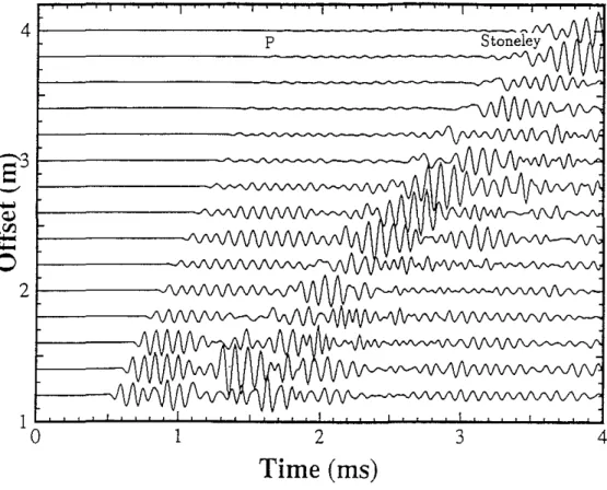
Figure 5a shows the synthetic array waveforms computed for a homogeneous forma-tion with the given Vp and V. values, and the random formations. For the

homoge-neous formation, the waveforms contain a P-wave train (its amplitude is too small to be visually seen at this scale), shear waveforms, Stoneley wave, and the very dispersive pesudo-Rayleigh waves. Because the large amplitude pseudo-Rayleigh waves move out across the array as the Airy phase, the shear wave train is clearly separated from the guided modes. Compared with the homogeneous case, the 10% random variation in Vp

and

V.

changes the shear wave amplitude characteristics. For the 15% variation, the changes are more significant (Figure 5c). For the homogeneous case, the shear wave amplitude systematically decreases across the array due to the

11

z2 geometric

spread-ing. For the random cases (especially the 15% case), the shear wave amplitude variation is random. It can decrease or increase with distance according to the local formation properties. This behavior poses a problem to the determination of shear wave attenua-tion in a heterogeneous formaattenua-tion using the shear wave amplitudes. The gUided modes are also affected by the scattering. The Stoneley mode becomes less coherent, largely because of the interference with the scattered waves. The pseudo-Rayleigh waves are affected to a lesser extent, because of their large amplitude and long duration.

V.

Variation Around

VI

The borehole guided waves, particularly the Stoneley waves, are very sensitive to the formation shear velocity. It is of particular interest here to study the effects of the variation of

V.

on the Stoneley waves. The critical sensitivity is around Vs

=

VI because the formation may be a fast formation if Vs

>

VI, and a slow formation if V.

<

VI' We therefore chose a mean value Vs

=

VI

=

1500

m/s.

The P-wave velocity

v".

and density are fixed at 3000

mls

and 2.4

g/cm

3

•

Figure 6a shows the synthetic array waveforms for homogeneous formation with the given Vp , V" and p values. The leaky-P and Stoneley waves are dominant phases in

the full waveforms. In Figure 6b, a 10% translational variation with correlation length equal to 0.1 m is added to Vs. The waveforms are very different from the homogeneous case (Figure 6a). The Stoneley wave becomes distorted because of scattering. Following the Stoneley waves, there are some resonant waves (e.g., at 3 m and 4 m locations), obviously due to the reverberation of Stoneley wave energy trapped by the local layering. In Figure 6c, a cyclic variation is used for the variation in Vs , in which V" = 1900

mls

and

v.,

= 1100

mls

(average value is 1500

m/s).

The average layer thickness is 0.1 m. For this cyclic variation, the Stoneley wave is distorted beyond recognization. The large amplitude events are probably due to the combination of pseudo-Rayleigh and Stoneley

energy trapped between the alternating high and low shear velocity layers. These waves attenuate very fast with travel distance and disappear beyond 3 m. In both Figure 6b and 6c, the leaky-P wave is the most coherent energy but their amplitudes are strongly affected by the shear velocity variation. These examples show that the shear velocity heterogeneity affects the behavior of guided modes, particularly when the

V.

is close to the borehole fluid velocity.

Effects of Layer Thickness

For the scattering of elastic waves in a random medium, the ratio of wavelength to the scale length of the random heterogeneities is an important parameter governing the wave characteristics. We study this effect using the cyclic random variation with different average layer thicknesses.

For the cyclic medium, we use V_P1

=

3200

mis,

V_P2

=

2000

m/s.

Vs and p are fixed at 1300

ml

sand 2.4 glcm3

, respectively. The case for the average layer thickness equal

to 0.1 m has been shown in Figure 3d. We now reduce the layer thickness by half, I.e.,

Ii

=

0.05 m. The corresponding formation model is shown in Figure 7. Figure 8 plots the computed waveforms. Compared with Figure 3d, the attenuation in the leaky-P wave train is much greater because the amplitude decays much faster than what is shown in Figure 3d. This can be explained using the different values of wavelength to layer thickness ratios. Previous examples showed that the P-wave train of the full waveform log can be approximated as a 1-D wave propagating along the borehole. Tang and Burns (1992) have shown that for 1-D scattering due to a layered random medium, the attenuation of the transmitted wave (I.e., the P-wave train in the present case) is peaked at

1

ka""

-2 (15)

where ais the correlation length of the random heterogeneities, and

k

=

2;

=

2:

1.

It has been shown that the cyclic random structure (e.g., Figure 1b) generated by Poisson distribution possesses an exponential correlation function with the correlation length equal to half of the average layer thickness (I.e., a=

~Ii,

see Jenkins and Watts, 1968). Therefore, for the cyclic random medium, the maximum attenuation will occur at

kli~1. (16)

kh ~ 1, meaning that the attenuation due to scattering is the strongest. While for Figure 3d, kh~ 2, which has lower attenuation than what we have seen in Figure 8.

Of special interest are the large amplitude events following the Stoneley waves. We interpret these waves as reverberations of Stoneley waves between layers. This happens when the average layer thickness

(ii

= 0.05 m) approaches the half wave length of the Stoneley wave (on the order of 0.06 m for the 10 kHz waves), the reverberation wave energy will interfere constructively, producing a wave traln whose wave length is approximately twice the average layer thickness. Therefore, the cyclic layer acts as a narrow band pass filter which selectively passes the waves whose wavelength is about twice that of the layer thickness. This phenomenon may be helpful in interpreting acoustic waveform logs measured in layered formations.

We now study the case where the layer thickness is greater than the wavelength. This case is modeled by changing the average layer thickness

h

in the previous example from 0.05 m to 0.5 m (Figure 9) and keeping other parameters unchanged. The synthetic waveforms are shown in Figure 10. Because in this case the variations are in the P-wave velocity, the P-P-wave train is greatly affected. The P-wave amplitude changes quasi-periodically because of the cyclic change of Vp with distance, with high amplitude

corresponding to high velocity (Vp,

=

3200 m/s) and low amplitude to low velocity

(Vp, = 2000 m/s) layers. Since the Stoneley wave is primarily controlled by V. (V. is fixed at 1300 m/s in this case) in a slow formation, its amplitude is not significantly affected.

As a last example, we show the effects of varyingV. on the Stoneley wave propagation in the borehole with a layered formation. The average layer thickness is

h

=

0.5 m. The shear velocity V. varies between

V.,'

=

1100 m/s and

11"

=

1900 m/s (Figure 11),

Vp

and p are fixed at 3000 m/sand 2.4 g/cm3, respectively. In order to show the Stoneley wave, we use a 5 kHz center frequency source. The synthetic waveforms are shown in Figure 12. Because the Stoneley wave is very sensitive to shear velocity, the Stoneley wave behavior is very different for receivers located in the V"

=

1100 m/s (slow formation) layer and those located in

V.,

= 1900 m/s (fast formation) layers. For waves received in the fast formation, the wave amplitudes are high, while for waves received in the slow formation, the amplitudes are very low. This behavior can be explained in terms of wave excitation in the fluid filled borehole surrounded by fast and slow formations (Tang and Cheng, 1993). In the fast formation, most of the Stoneley wave energy is concentrated in the bore fiuid. For a receiver in the borehole, the received wave amplitude should be high. In the slow formation, a significant portion of the Stoneley wave energy is contained in the formation. Therefore, the energy in the bore fluid is much reduced compared to the fast formation case, thus having a much lower amplitude. In addition, the radiation loss at the layer boundaries is also evident. For example, the wave amplitude at 3.5 m is much reduced compared to that at 1 m (both are within fast formation). The examples shown in Figures 10 and 12 indicate that for

a heterogeneous formation, the recorded wave amplitudes (be they Stoneley or leaky-P) are strongly controlled by the local formation properties of the receiver position.

CONCLUSIONS

In this study, acoustic wave propagation in a fluid-filled borehole surrounded by a ran-domly stratified formation variation has been investigated using the finite difference technique. The random variation of formation properties along the borehole can have significant effects on the wave propagation characteristics, resulting in scattering and ar-rival time delay of the propagating waves. For the P- and S-wave arar-rivals, the waves can be regarded as being composed of two parts, the coherent part (transmitted waves) and the incoherent part (scattered waves). The coherent part of the waves can be processed using conventional techniques to obtain formation velocity, although the accuracy of this velocity relative to the true formation average velocity is subject to the degree of variation of formation heterogeneity. The wave amplitudes are also attenuated because of the scattering. The attenuation is dependent on the wavelength relative to the scale length of the heterogeneities. For the guided waves (such as Stoneley waves), the wave amplitude is primarily controlled by two factors; one is the local formation properties which determine the wave excitation condition for the receiver location, the other is the scattering and radiation losses along the path from source to receivers.

ACKNOWLEDGEMENTS

This research was supported by the Borehole Acoustics and Logging Consortium at M.LT., and by New England Research.

REFERENCES

Biot, M.A., 1952, Propagation of elastic waves in a cylindrical bore containing a fluid,

J. Appl. Phys., 23,977-1005.

Cheng, C.H., and M.N. ToksQz, 1981, Elastic wave propagation in a fluid-filled borehole and synthetic acoustic logs, Geophysics, 46, 1042-1053.

Frankel A., and RW. Clayton, 1986, Finite difference simulations for the propagation of short-period seismic waves in the crust and crustal heterogeneity, J. Geophys. Res.,

91, 6465-6489.

Jenkins, G.M., and D.G. Watts, 1968, Spectral analysis and its applications, Holden-Day, San Francisco.

Kerner, C., 1992, Anisotropy in sedimentary rocks modeled as random media,

Geo-physics, 57, 564-576.

Kostek, S., 1991, Modelling of elastic wave propagation in a fluid-filled borehole excited by a piezoelectric transducer; Master thesis, Massachusetts Institute of Technology, Cambridge, Massachusetts.

O'Doherty, RF., and N.A. Anstey, 1971, Reflection on amplitude, Geophys. Prosp., 19, 1-26.

Stewart, R.R, P.D. Huddelston, and T.K. Kan, 1984, Seismic versus sonic velocities: a vertical seismic profiling study, Geophysics, 49, 1153-1168.

Tang, X.M., and D.R Burns, 1992, Seismic scattering and velocity dispersion due to heterogeneous lithology, SEG 62nd Annual International Meetin9 and Exposition,

Expanded Abstract, New Orleans.

Tang, X.M., and C.H. Cheng, 1993, effects of a logging tool on the Stoneley waves in elastic and porous boreholes, The Log Analyst, 34, in press.

Virieux, J., 1986, P-SV wave propagation in heterogenous media: velocity-stress finite-difference method, Geophysics, 50, 1588-1609.

4 10002000300040005000

VELOCITY

(m/s)

b. Cyclic

5

-y---==---,

4

o-+---,--r-r-r=t----r-.--j

1000 2000 3000 4000 5000

VELOCITY

(m/s)

5 - r - - - - . , , - - - ,

a. Translational

--.

.-...

_E

E

₃

~

3

" - '

w

w

(J (J

z

:z

_c::r

c::r

₂

l-I- (J)

2

(J)

-Cl Cl

1

₁

Translational

Cyclic 1

Cyclic 2

I I I

2000 3000 2000 3000

P·WAVE VELOCITY (mis) P·WAVE VELOCITY (mls)

2000 3000 P·WAVE VELOCITY (m/s) E ~ 3 1IJ U Z <t I-

-en

2 \ 0

-Figure 2: Translational and cyclic (1 and 2) formation models for computing synthetic borehole acoustic waveforms. Note that the deviation (from mean) of cyclic model 2 is twice that of cyclic model 1.

2 Time (ms) 4 4 3

,"

"

2

_"

i:'-"

,

v ,

"

' ';A',', :

...

_.A

_".v,"

,l,"'...A '" ,AIIIINA',

'V"',"

:

'0

:§:3

~

'"

il!

o

2 c, d. 2 Time (ms) o 4 _{P Stoudey} 3

",

,ii, ~,','" 2

_,

,,"

_A~

.v

,

, 4 ':. 3

'"

2 "'A "v,VN.'.':·· .

~.

,

, 4

.,

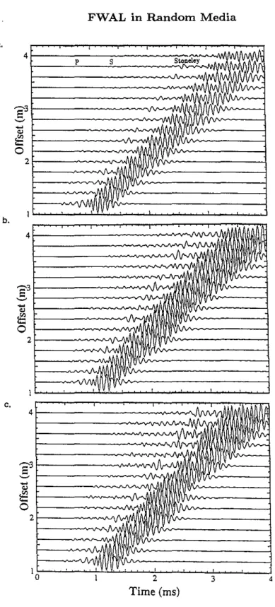
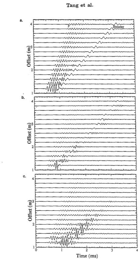
b,

Figure 3: Simulated full waveform acoustic logs for (a) homogeneous, (b) translational, (c) cyclic 1, and (d) cyclic 2 formation models shown in Figure 2.

Effects of Heterogeneity Scattering on First Arivals

- - - homogeneous - translational - - - cyclic 2 ... - ... -. cyclic 1 I---~~...,..,.~ - '-1.5 1.6 Time (ms) 1.7 1.8

Figure 4: Overlay of first arrivals of P-wave train at 4 m from source for Figure 3a, b, c, and d. Note the amplitude reduction and travel time delay of the heterogeneous model results relative to the homogeneous model result.

4 3 2 Time (ms) ~ p S Stoudey

Wi

.:,

,r

,,'

,Vj',

:,',V,I

JV

'.v.

v ' ~:: IV :

..

;

":i~V,V,V.I ~::i~VjV,VV

,

JVV

·~

..m',v.'

IV "1'i~\I\I\I' ... KlVAVJlVV 1 'v

v',VVVV

4r---~Jv-v"'_./V'fV\.~LMI\1 4

'53

f---Jo-"'-"MI"IiI\,-'JI.,fII,lVl~ ~ r----~~.-.Aj1N\/1IN 1I'1l'i\N----I

-

_'"

lJ9

'----o/V"~~~II"""M

o

I---~~"""'I\IVI,\\I!M 21----~J'./\,'lAI~fiI E31---~~-v-J\fIrMIWV\ll ~ ~rl.r~-_ _1

-

_'"

~

..

o

2'----~'_JV\rvWiJ\~ c. b. a.

Figure 5: Synthetic waveform logs for 10 percent (h) and 15 percent (c) translational variation in

v,.

and

v,.

The homogeneous model result is also shown (a).

4 3 2 Time (ms) 4 4 p _Stoneley

.

A ,"

''',

-~~i.;.' ; , ' , >V 1m"( 1 "V }I",

"'

..

,,n, "

"VV , -, .• :K. "lK"'.V " .,,',':fiA"VY " •• ,',': -vUv, '~v:":.mr.' V,'vvV' _, 4 c. b. a.

Figure 6: Effects of heterogeneity variation of Vs around VI' (a) homogeneous model with

V.

= VI; (b) translational model; and (c) cyclic model.

w

U

z

«

....

en

Cl 4 3 2 1

a

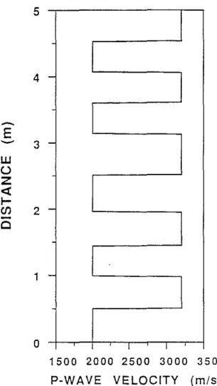
1500 2000 2500 3000 3500 P-WAVE VELOCITY (m/s)

Figure 7: Cyclic model obtained by reducing the average layer thickness of cyclic model 2 in Figure 2 by half.

41---=---~_:_.

1

2

Time (ms)

3 4

Figure 8: Synthetic waveform log for the formation model in Figure 7. Note the strong attenuation of the P-wave train and the reverberations folowing the Stoneley wave arrivals.

w

U Z ~

I-en

Cl 5 4 3 2 1

o

-I I 1500 2000 2500 3000 3500 P-WAVE VELOCITY (m/s)

Figure 9: Cyclic formation model (for P-wave velocity). The layer thickness is greater than the wavelength of study.

4 1 - - - J \ / \

p

8'3

f - - - -J_\!\

...

dol

~

o

2 1 - - - . 1 St 1o~

...

..l.I...2~...l.3...4

Time

(ms)

Figure 10: Computed waveform log for the model in Figure 10. The P-wave amplitude changes periodically between the layers.

UJ () Z <t

....

en

Cl 5 4 3 2 1

o

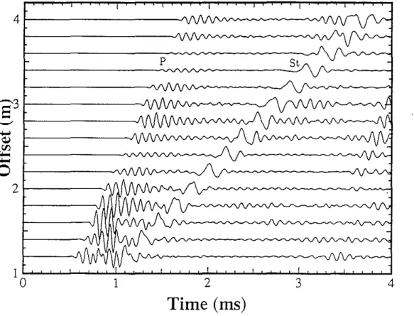
-I I I I 500 1000 1500 2000 2500 S-WAVE VELOCITY (m/s)

Figure 11: Cyclic formation model (for S-wave velocity). The layer thickness is greater than the wavelength of study.

4 \ \ I

,

P St09;eley ~ ~ ~ ~ ~ ~

~~

\i

,

, 1 2

Time (ms)

3

4

Figure 12: Computed waveform log for the model in Figure 11 (source center frequency is 5 KHz). The Stoneley wave amplitude changes dramatically between low- and high-velocity layers.