Lame ducks and divided government: How voters control the unaccountable

Contents lists available at ScienceDirect

Journal

of

Comparative

Economics

journal homepage: www.elsevier.com/locate/jce

Lame

ducks

and

divided

government:

How

voters

control

the

unaccountable

R

Mark

Schelker

University of Fribourg, CESifo and CREMA, Bd. de Perolles 90, 1700 Fribourg, Switzerland

a

r

t

i

c

l

e

i

n

f

o

Article history:

Received 13 November 2015 Revised 21 February 2017 Accepted 21 February 2017 Available online 22 February 2017 JEL classification: D72 Keywords: Divided government Lame duck Term limit

a

b

s

t

r

a

c

t

Schelker, Mark —Lameducksanddividedgovernment:Howvoterscontrolthe unaccount-able

Electoralinstitutions interact throughtheincentives they providetopolicy makers and

voters.Inthispaperdividedgovernmentisinterpretedasthereactionofvoterstoa sys-tematiccontrolproblem.Votersrealizethatterm-limitedexecutives(“lameducks”)cannot crediblycommittoamoderateelectoralplatformduetomissingreelectionincentives.By

dividinggovernmentcontrolvotersforcealameducktocompromiseonpolicieswithan

opposinglegislature. BasedondatafromtheUSstates, Ipresentevidenceshowingthat

theprobabilityofdividedgovernmentisabout8to10percenthigherwhengovernorsare

lameducks. JournalofComparativeEconomics 46 (2018)131–144. UniversityofFribourg, CESifoandCREMA,Bd.dePerolles90,1700Fribourg,Switzerland.

© 2017AssociationforComparativeEconomicStudies.PublishedbyElsevierInc.Allrights reserved.

1. Introduction

Electoral institutions define the rules and structures of interactions between voters, politicians, and parties. Rational indi- viduals optimize within this set of rules. The various institutions interact through the incentives they provide to individuals. It is from this perspective that I analyze two important phenomena in the political system of the USA: divided government and term-limited and thus unaccountable politicians. I argue that divided government can serve voters as a mechanism to moderate term-limited executives (henceforth “lame ducks”) who are otherwise unaccountable and who cannot credibly commit to a moderate policy platform due to their lack of electoral incentives. A divided government forces lame ducks to compromise on policy with an opposing legislature. In the empirical analysis, I study whether there is a higher probability of divided government in office terms when the executive term limit is binding; that is, when the executive is a “lame duck”.

In a series of empirical specifications I attempt to identify the causal effect of lame duck governors on the occurrence of divided government in US states. First, I estimate standard panel data models including state and year fixed effects. Second, I focus on selection and last-period effects as potential confounding factors. Third, I take advantage of close elections

R I would like to thank Jim Alt, Christine Benesch, Nels Christiansen, Reiner Eichenberger, Jürgen Eichberger, Bruno Frey, Roland Hodler, Mario Jametti,

Marcelin Joanis, Fabien Moizeau, Susanne Neckermann and Andrei Shleifer for helpful comments and discussions. The paper also greatly benefited from comments by seminar participants at the Universities of Fribourg, Heidelberg, Lausanne, Lugano, Mannheim, and St. Gallen and by conference participants of the North American Summer Meeting of the Econometric Society in St. Louis, the International Society for New Institutional Economics at Stanford, the World Congress of the International Economic Association in Beijing, the International Institute of Public Finance at Ross School of Business in Ann Arbor, the European Economic Association in Oslo, the European Public Choice Society in Rennes, the CESifo Area Conference in Applied Microeconomics in Munich, and the European Political Science Association in Berlin.

E-mail address: mark.schelker@unifr.ch http://dx.doi.org/10.1016/j.jce.2017.02.005

and implement an approach which is similar in spirit to a regression discontinuity design. Fourth, I explore various other mechanisms that might affect the occurrence of divided government. Over all specifications, I find robust evidence that lame ducks face an approximately 8 to 10 percent higher probability of divided government.

Section2presents the major arguments of two hitherto separate literatures and discusses the main mechanism through which divided governments and binding term limits interact. Section 3 introduces the data and the empirical strategy. Section4reports the empirical results. Section5concludes.

2. Dividedgovernment:thereactionofvoterstoasystematiccontrolproblem

To provide a foundation for the main argument that voters divide government power to control an unaccountable lame duck, I briefly introduce the main arguments and mechanisms established in two relevant literatures.

2.1. Causes of divided government

Divided government is a common phenomenon in presidential systems in which the executive and legislative branches are elected separately by voters. A prime example is the political system of the United States with its two main parties, the Republican and Democratic Parties. At the federal level, divided government was the dominant form of government during the period from 1952 to 2010. Approximately 59 percent of all the governments were divided in the sense that the Presidency and the Federal Congress – the Senate and/or the House of Representatives – were dominated by opposing party majorities.

Fiorina (1992)and Alesina and Rosenthal (1995, 1996) analyze the causes of divided government in a spatial voting framework and argue that the division of government control is the result of rational voter behavior. Fiorina puts forward “balancing explanations” of divided government, in which voter decisions have “[…] an element of purpose or intention in them.” ( Fiorina, 1992: 65). He proposes the idea that divided government is the electoral result of rational decisions by moderate voters who balance political power between opposing party ideologies to moderate policy outcomes. Hence, voters at the center of the policy spectrum moderate policy by electing different parties into the branches of government. This requires sophisticated voters who understand the institutional setup, enabling them to make use of the extensive checks and balances inherent to a system with such a strong separation of powers. Similar in spirit to Fiorina(1992),Alesina andRosenthal (1995,1996) build a formal model that extends the standard spatial voting theory to include the separate election of the executive and legislative branches with the possibility of dividing government control. In their model, policy is viewed as a compromise between the executive and the legislative branch. When both branches are held by one party – known as unified government – the party in power can implement its preferred policy. When the branches of government are dominated by different party majorities, the opposing parties in the different branches become veto players and they are forced to compromise on policy. Voters whose positions fall between the preferred party positions take advantage of this legislative–executive interaction to moderate policy outcomes. The mechanism relates directly to the fundamental concept of the separations of powers, in which, by the design of appropriate checks and balances, a conflict of interest is created and the executive and the legislative branch are required to compromise ( Perssonetal.,1997). AlesinaandRosenthal(1995) argue that divided government “[…] is not an undesired result of a cumbersome electoral process, nor is it the result of a lack of rationality or of well-defined preferences of the electorate. Divided government occurs because moderate voters like it, and they take advantage of “checks and balances” to achieve moderation. In dividing government, the voters force the parties to compromise: divided government is a remedy of political polarization” ( AlesinaandRosenthal,1995: 44). 1

Their formal model is consistent with three important empirical observations: divided government, split-ticket voting, and the midterm cycle. The theory predicts divided government as an outcome of voters’ strategic electoral balancing of party ideologies in government, in which moderate voters split their tickets. In general elections, when the executive and (partly) the legislative are simultaneously elected, voters are uncertain about which party will be holding the executive. Voters who want to moderate policy by dividing government will therefore hedge the legislature by dividing power between the legislative branches. Once the uncertainty about the incumbent party in the executive is resolved, voters might want to moderate the government in midterm elections further by shifting even more legislative power to the opposition party. This results in the well-documented midterm cycle.

2.2. Term-limited executives and electoral accountability

Regular elections make politicians respond to citizens’ preferences, which makes it the prime democratic channel through which citizens can hold politicians accountable (e.g., Alt et al., 2011). From this perspective, introducing term

1 Fiorina’s argument is not based on active moderating behavior. Under the assumption of sincere voting, moderate voters divide government power

because divided governments offer policies closer to their bliss points compared to unified governments. In contrast, the argument by Alesina and Rosenthal (1995 ) is based on an active strategic moderation effort of voters (for evidence on balancing behavior, see Mebane 20 0 0 and Mebane and Sekhon 2002 ). The basic idea that voters actually choose divided government is inspired by the well-documented phenomenon of split-ticket voting. For evidence of split- ticket voting, see, e.g., Fiorina (1992) and Burden and Kimball (2002) . An alternative model of split-ticket voting is provided by Chari, Jones and Marimon (1997) .

limits and thus limiting electoral incentives seems controversial at first sight. However, there are at least two simultaneous effects that have to be taken into account: On the one hand, term limits reduce office tenure in expectation and, hence, may increase political competition (e.g., Daniel andLott,1997), or reduce the rent-seeking and limit the political power of long-term incumbents (e.g., DickandLott,1993; FriedmanandWittman,1995). On the other hand, the major disadvantage of term limit legislation stems from the last period in office when the term limit is binding and the executive becomes a “lame duck” ( Barro, 1973). 2 _{Executives who care about maintaining a reputation for the purposes of being re-elected} must introduce policies that are in accordance with voter preferences. Being ineligible to run for reelection eliminates this powerful incentive. In both, spatial voting models as well as political agency models, electoral incentives are the main channel through which to align the preferences of the officeholder with those of the voters. The lack of accountability to voters increases a politician’s incentives to engage in opportunistic behavior, which could manifest, e.g., in ideological deviation, low levels of effort, activities that favor personal interests, outright corruption or legacy building (e.g., Besleyand Case,1995; ListandSturm,2006; FerrazandFinan,2011). 3

One obvious question is why voters actually re-elect a governor into a lame duck term, especially if moral hazard becomes an issue, i.e., an officeholder cannot credibly commit to a moderate electoral platform. By backward induction it becomes apparent that if voters commit to not re-electing an incumbent into the last lame duck term, the governor actually becomes a lame duck already in the previous period. Hence, a term limit in whatever future term would factually be reduced to a one-term limit ( Altetal.,2011).

2.3. How voters use divided government to control lame ducks

The policy balancing behavior of moderate voters ( Fiorina, 1992; Alesina and Rosenthal, 1995, 1996) must not be restricted to balancing party ideology in legislative and executive elections. Voters might also use the mechanism to counteract specific accountability problems. If voters realize that providing veto power to different party majorities in the executive and the legislative forces the different ideologies and interests to compromise, they may also realize that they can use this mechanism to mitigate other control problems. One such example is the lack of reelection incentives of term- limited executives in the last period of their mandate. Term-limited executives do not face a reelection constraint which can result in serious moral hazard and an inability to commit to a moderate electoral platform. ListandSturm(2006)show that lame duck governors deviate from their previous political positions. 4 _{Voters anticipate the weakened incentives of a} term-limited executive to remaining close to the preferences of the electorate rather than deviating to implement policies in line with personal ideological preferences. They use the electoral mechanism by voting for the opposing party in the legislative branch in an attempt to divide government control. Divided government provides veto power to the opposing party and forces a lame duck executive to compromise on policy matters.

However, policy moderation by means of divided government may come at a cost: if the different parties in the executive and legislative branches cannot compromise on policy, this may lead to gridlock in the policy making process, obscure ac- countability, and hold up policy reactions to economic shocks (e.g., Sundquist,1988; CoxandMcCubbins,1991; McCubbins, 1991; AltandLowry,1994; Poterba,1994). Mayhew(1991)argues that in terms of “significant” legislative enactments, there is no evidence of policy stalemates in the United States. However, it has been shown that the evaluation of the effect of divided government on legislative productivity depends heavily on the definition of “significant” enactments, the definition of gridlock, as well as additional factors such as party polarization and inner-party ideological heterogeneity (e.g., Krehbiel, 1996; Binder,1999; Coleman,1999; Howelletal.,2000; BowlingandFerguson,2001; Jones,2001; Rogers,2005; Saeki2009).

Hence, the decision to moderate policy by means of divided government depends on the relative cost of divided govern- ment. Voters must weigh the cost of potential policy gridlock against the cost of a lame duck wielding executive powers. If the expected costs of divided government are lower than the expected costs of having a lame duck, then voters can opt for policy moderation by dividing government control. While the deviation from the previous term’s politics of lame duck executives is well established, 5 _{the cost of policy making under divided government remains ambiguous. In the empirical} analysis, I attempt to control for the alleged drivers of the cost of divided government and I include party ideology and ideological heterogeneity into the econometric framework. Failing to fully control for the cost of divided government should

2 Note that in line with the previous literature (e.g., _{Barro 1973 ) I will generally refer to governors facing a binding term limit as “lame ducks”. This}

is not meant as any particular qualification of term-limited governors’ behavior. It is conceivable that term-limited and thus unaccountable officeholders become more ideological, reduce effort, or invest more in acquiring private rents, but they might also become more independent from party or special interests and invest more in the provision of public goods, and so on. The main point is, however, that lame ducks are prone to deviate from their previous positions and that voters are uncertain of how they will deviate.

3 Much of the term limit literature uses the agency framework to model the behavior of officeholders in their lame duck term. There, electoral ac-

countability comes from the reelection constraint which incentivizes officeholders to cater to citizens preferences. In the agency literature this incentive channel determines the effort of the officeholder. Effort, however, can take different forms. A lack of reelection incentives can induce low effort (i.e., make incumbents lazy), make them corrupt, or more partisan. Again, the essential point is that term-limited officeholders can deviate from first term policies.

4 Besides the standard theoretical prediction from spatial voting theory there is substantial empirical evidence that elected policymakers tend to deviate

from the preferences of the electorate when electoral competition is less intense and hence, less constraining (e.g., Ansolabehere et al., 2001 ; Canes-Wrone et al., 2002 ; List and Sturm, 2006 ; Snyder and Strömberg, 2010 ).

5 Note that for the main argument it suffices that lame ducks deviate from previous term behavior and voters are uncertain about the direction of the

Table 1

Gubernatorial term limits in the US states. Term limits for governors by state (1970–2010) States with no term limits:

CT, ID a_{, IL, IA, MA} b_{, MN, NH, NY, ND, TX, VT, WA} c_{, WI, UT} e States limiting governors to one term in office:

VA d

States limiting governors to two terms in office:

AL, DE, FL, LA, MD, ME, MO, NE, NJ, NV, OH, OK, OR, PA, SD, WV State law changed from no term limit to a two-term limit:

AZ (1992), AR (1992), CA (1990), CO (1990), KS (1974), MI (1992), MT (1992), RI (1994), WY (1992) State law changed from a one-term limit to a two-term limit:

GA (1976), IN (1972), KY (1992), NM (1991), MS (1986), NC (1977), SC (1980), TN (1978) Source: List and Sturm (2006), own update after 20 0 0.

Note: The year in brackets is the year in which the term limit legislation changed.

a A two-term limit was passed in 1994 but repealed in 2002 by the Idaho State Legislature.

b Term limits were enacted in 1994 but were declared unconstitutional by the Massachusetts Supreme Court in 1997. c Enacted a two-term limit in 1992, which was declared unconstitutional by the Washington Supreme Court in 1998. d Restrictions on terms enacted in 1954.

e A three-term limit was passed in 1994 and repealed in 2003 by the Utah State Legislature.

result in downward bias of the coefficient of interest and make it more difficult to find a systematic relationship between lame ducks and divided government.

The underlying mechanism leading to divided government is based on the number of seats in the legislature. Therefore, it could also be interesting to analyze whether the anticipated effects are also observable in the underlying distribution of legislative seats. I expect that the party of the governor loses seat shares in the lame duck term. However, the main hypothesis of this contribution is based on a requirement of two opposing veto players to compromise over policy in the two branches of government. This situation is effectively achieved by a divided government. The veto power leading to policy moderation is a discontinuous function of the distribution of seats in the legislature. Hence, the main focus of the empirical investigation is on divided government and the (consistent) empirical evidence based on legislative seat shares is relegated to the Online Appendix.

Based on spatial voting theory, voters divide government power to prevent lame duck incumbents from implementing extreme partisan policies. Pure lack of effort (which is the main mechanism in agency theory) cannot be prevented by dividing government power. Overall, I expect to observe an increase in the probability of divided government for governors in their lame duck term.

3. Dataandempiricalstrategy

In line with the previous literature, I use data for the 48 US mainland states from 1970 to 2010. The US states are an ideal testing ground on which to assess these theoretical predictions. First, many US states have implemented executive term limits. Out of the 50 states, 37 feature binding executive term limits in 2010, many of which were introduced following voter initiatives. During the period of this study, on average 27 percent of governors were lame ducks. Table1 provides an overview of the executive term limit legislation in each state. Second, the executive and legislative branches are both elected directly by citizens. At the US state level, divided government occurred 50 percent of the time during the period from 1970 to 2010.

3.1. The data

The information pertaining to party majorities in the branches of government for the period from 1970 to 20 0 0 is primarily based on Alt et al. (2006), from 20 0 0 to 2010, the information stems from the National Conference of State Legislatures (NCSL). The data include information regarding the parties holding the executive and the majorities in the two legislative chambers. The dependent variable is an indicator variable that takes the value 1 when there is any form of divided government (and parties need to compromise), whether it is divided between the executive branch and both chambers of the legislature or the majorities are split in the legislative chambers. Up to the year 20 0 0, the bulk of the independent variables stems from ListandSturm(2006). They provide information on state executive term limit legislation (see Table1), term-limited governors (lame ducks), and the electoral margin of incumbent governors relative to the main challenger as well as economic and socio-demographic characteristics. 6 _{From 20 0 0 onwards, I collect the information on} term limits, lame ducks, elections years, etc. from the official state sources. I calculate governors vote margins based on the data provided by Leip(2015). Information pertaining to the timing of legislative elections in each state was provided by

6 I cross-checked and, if necessary, corrected the data used in this study with the (original) data source by _{Besley and Case (2003) and the later relevant}

Tim Storey from the National Conference of State Legislators (NCSL). Appendix TablesA1and A2present summary statistics and information on the the data sources. 7

3.2. Empirical strategy

The empirical strategy aims at identifying the effect of lame ducks on divided government. Therefore, it is important to separate the specific lame duck effects that are caused by the inability to run for the same office in the next election, from the direct effect of term limits such as increased political competition or a reduction of incumbency advantages. Because I am interested in the lame duck effect, I have to control for the direct effect of term limits or, alternatively, focus on subsamples.

The following empirical analysis starts by establishing baseline estimates that focus on the main variables of interest only. Then I extend the framework by analyzing specific channels to eliminate potential sources of bias such as gubernatorial experience due to electoral selection ( Altetal.,2011) and general last-round effects that may also affect governors not facing a term limit. I complement these results with estimates based on close elections, in the spirit of a regression discontinuity design. In a last step, I control for further covariates that potentially affect the occurrence of divided government.

I estimate variants of the following panel specification:

yit =

β

ζ

λ

μ

τ

ε

y it is a dummy variable capturing the form of government (1 if divided government, 0 if unified government) in state i

in year t. lame duck it is a dummy variable that takes the value 1 if the executive is a lame duck and 0 otherwise. Iit is

a vector that includes potentially important institutional and gubernatorial characteristics (e.g., term limit, vote margins, midterm congresses), and Xit is a vector of additional controls (e.g., political and preferences variables).

β

of interest,

ζ

λ

μi

τ

εit

subscripts i = 1,…, n and t = 1,…, T indicate the state and year, respectively.

Given the binary dependent variable, natural specifications include linear probability models and non-linear models such as logit or probit. The presented results in this text are primarily based on linear probability models, which are typically good approximations, simple to interpret, and widely used in economic research. Fixed effects logit estimates are presented in the baseline regressions ( Table 2) and in the Online Appendix afterwards. 8 _{Because panel data estimates might ignore} autocorrelation in US state data ( Bertrandetal.,2004), I adjust the standard errors for clustering at the state level, which allows for arbitrary correlations of the errors within states. 9

The main attention is on identifying the effect of lame duck governors on the occurrence of divided government. Because lame ducks do not occur randomly, I control for the two main factors determining whether a governor can actually become a lame duck: that is, for whether there is a term limit and for the governor’s vote margin in the last election leading to its concurrent office term. Term limits were not introduced with the main intention of creating an unaccountable last term but, instead, to reduce the perceived negative effects of long term incumbents. Therefore, term limit legislation per se might have an independent effect. For identification, it is thus important to separate these potentially divergent effects. The concurrent vote margin of an incumbent governor is important from two perspectives: First, it captures the popularity of an incumbent or candidate relative to the popularity of a challenger in the last electoral race. One could expect that more popular candi- dates or incumbents with higher vote margins should face a lower probability of confronting an opposing party majority in the legislative branch. Second, the concurrent vote margin should be an unbiased ex-ante indicator of the predictability of the (re-)election of a candidate, which influences the ability of voters to effectively moderate policy by dividing government control. From this perspective a higher vote margin could also increase the probability of divided government.

I expect the lame duck coefficient to be positive. For the term limit variable, I do not have an a priori hypothesis regarding the direction of the overall effect. From a theoretical perspective also the direction of the effect of the vote margin is ambiguous: Larger vote margins might indicate popular candidates that face lower probabilities of divided government, at the same time it improves voters’ ability to effectively divide government because there is a lower uncertainty about who will be elected to the gubernatorial office. It is an empirical question which effect dominates.

Because not all states follow identical electoral systems and electoral rhythms, I control for the electoral cycle and I include an indicator identifying midterm congresses . Likewise, this allows me to evaluate potential midterm dynamics (e.g., AlesinaandRosenthal,1996; FolkeandSnyder,2012). I exclude observations from the few states (for some period of time) that limit governors to one term in office only, which makes all governors lame ducks at all times.

The empirical strategy develops as follows: first, I present the simplest possible specifications establishing the baseline results (4.1.). Second, I eliminate specific channels, introducing potential bias due to electoral selection and experience as well as general last-round effects (4.2.). Third, I focus on closely elected governors and implement specifications based on the idea of a regression discontinuity (4.3.). Fourth, I conduct a series of robustness checks by introducing covariates ap- proximating political preferences, preference heterogeneity, political polarization, party affiliation, and presidential coattails – all of which may influence the results (4.4.).

7 Table OA.1 of the Online Appendix presents yearly summary statistics of the main variables of interest.

8 All results from the conditional logit regressions are consistent with the results of the linear regressions (see Online Appendix). 9 The results also remain robust to the inclusion of state-specific time trends (not reported).

Table 2 Baseline results

Dependent variable: divided government.

(1) (2) (3) (4)

OLS OLS LOGIT LOGIT

Lame duck 0.094 ∗∗ _0.094 ∗∗ _0.469 ∗∗ _0.469 ∗∗ (0.043) (0.043) (0.212) (0.212) [0.107] ∗∗ _[0.105] ∗∗∗ Term limit −0.130 −0.133 −0.663 −0.672 (0.121) (0.120) (0.548) (0.545) Vote margin −0.012 ∗∗∗ _−0.012 ∗∗∗ _−0.060 ∗∗∗ _−0.060 ∗∗∗ (0.003) (0.003) (0.016) (0.016) Midterm 0.025 0.117 (0.019) (0.088)

State FE yes yes yes yes

Year FE yes yes yes yes

Observations 1761 1761 1761 1761

(pseudo) R-squared 0.058 0.058 0.053 0.053 Note: Standard errors are adjusted to within-state clustering and reported in parentheses. Marginal effects are reported in brackets. Significance level:

∗_{0.05 < p < 0.1,} ∗∗_{0.01 < p < 0.05,} ∗∗∗ _{p < 0.01.} 4. Empiricalresults

4.1. Baseline results

Columns 1 and 2 of Table2report the regression results from the linear probability models, and columns 3 and 4 report the results from fixed effects logit models. Columns 1 and 3 report results of a baseline specification just including the three previously discussed variables lame duck, term limit and vote margin . Columns 2 and 4 further control for potential legislative shifts after midterm elections. All presented specifications include state and year fixed effects.

4.1.1. Lame ducks

The lame duck coefficient is in all specifications positive and statistically significant, indicating a 9 to 10 percent higher probability of divided government if the term limit is binding. 10 _{The term limit variable has a sometimes marginally} significant negative effect on divided government (more extensive discussion below). The concurrent vote margin has a negative and significant impact on divided government, suggesting that more popular governors have a lower probability of confronting an opposing congress.

Overall, I consistently find that lame duck governors are associated with a significantly higher probability of divided government. 11 _{This finding is in line with the prediction that the impaired accountability of a lame duck increases the} inclination of voters to counterbalance this control problem by voting for divided government. In the linear regressions, the size of the coefficients suggests a 9 percent, and the marginal effects of the logistic regressions suggest a 10 percent higher probability of divided government when a governor is a lame duck. When analyzing the impact of lame ducks on the underlying legislative seat shares, I consistently find a negative and oftentimes (marginally) significant effect. The effect amounts to an approximately 3 percent loss in legislative seat shares for the party associated with a lame duck executive (for the full set of results, see the Online Appendix).

4.1.2. Term limits

I find a rather robust (though mostly insignificant) negative correlation between term limit legislation and divided government. This might suggest that term limits have an effect that goes beyond just introducing a last unaccountable term. Note that a direct interpretation of the estimated term limit coefficient per se is not possible. However, based on the literature pertaining to term limits, several interpretations could apply. E.g., term limits eliminate incumbency advantages after a few periods in office and the lack of such advantages increases electoral competition (e.g., Daniel andLott,1997).

10 Specifications not including fixed effects produce qualitatively similar results. It is comforting that the estimated coefficients do not depend on whether

linear or non-linear models are estimated, or whether just within or also cross-sectional variation is used for identification.

11 Subsamples: In Table OA.2 of the Online Appendix I report regression results focusing on specific subsamples. First, I restrict the sample to only include

years after general or midterm elections. One concern could be that the full sample of years between 1970 and 2010 could yield biased estimates because all congress years are included in the sample. The reason for the inclusion of all years in the baseline specification is primarily to keep the panel balanced because the states follow different electoral cycles. Despite the reduced sample size, the results based on the restricted sample remain almost identical (Table OA.2, columns 1–2). Second, I use only the subsample of states with term limit legislation (Table OA.2, columns 3–4). A potential concern could be that term limit states are different from non-term limit states and that this difference is not controlled for by the term limit variable. I consistently find positive and significant effects of the lame duck variable, which indicate a 9 to 12 percent higher probability of divided government. The magnitude of the effect is slightly higher but still comparable in size to the estimates that include the full sample of states.

Alternatively, term limits might enable voters to exchange long-term incumbents while keeping the same party in the executive. This ability may suit the interests of voters if incumbents tend to accumulate power over time and increasingly shirk or become corrupt with longer tenure. Moreover, term limits may be favored because they enable voters to anticipate last-round effects and coordinate their moderation effort s to the specific lame duck term. Without term limits, voters remain uncertain regarding which term is a governor’s final term, in which reelection incentives do not apply. Voters might be induced to hedge constantly against the risk of the incumbent’s moral hazard in a potential last-round term. Even other interpretations might apply and it is impossible to pin down the exact mechanism in our context. Note that without controlling for term limits the lame duck coefficient remains significant with an effect of 7 percent.

4.1.3. Electoral dynamics in midterm elections

When faced with greater uncertainty regarding who will be holding the executive office, voters may find the task of moderating policy by means of divided government more difficult. Alesina and Rosenthal (1996) argue that in general election years with great uncertainty about which party will be holding the executive, voters who want to moderate policy by dividing government will hedge the legislature by dividing power between the legislative branches. Once the uncertainty about the incumbent party in the executive is resolved, voters might want to moderate the government in midterm elections further by shifting even more legislative power to the opposition party. This results in the well-documented midterm losses of the party holding the executive. FolkeandSnyder(2012)analyze gubernatorial midterm slump and show that, in midterm elections, the party of the governor experiences an average seat share loss of about 3.5 percent. Such dynamics might also be observable in our setup. The results presented in Table 2 show that midterm congresses per se do not seem to have a significant influence on the probability of divided government. Table OA.7 in the Online Appendix shows that a party loses about 3 percentage points in legislative seat shares when the governor is a lame duck and about 1.4 percentage points in midterm congresses . It shows that there are some electoral dynamics in the underlying seat shares but that they are not sufficient to tip the balance to divide government power.

4.2. Selection of governors

A major concern could be that lame duck governors are of a particular selection of incumbents. In that case it might not be the fact that the governor is a lame duck and that voters anticipate a moral hazard problem, but some characteristic not particularly related to lame duck governors that drives the results.

4.2.1. Office terms, governor experience, and career concerns

So far, I have mainly suggested the moral hazard channel due to the missing accountability of a term-limited executive without reelection incentives. However, lame duck governors are re-elected and thus, selected and experienced executives. On average, lame ducks may be of higher quality than newly elected governors, because they have been re-elected and elections weed out incompetent incumbents (e.g., Alt et al., 2011). Alternatively, voters might just become weary of long-term governors and hence might want to restrict governors’ influence over public policy. To identify the influence of the missing accountability, I control for selection and competence effects ( Table3, columns 1 to 3). I first control for the number of terms in office ( # governor terms ) and proceed to include a flexible form of controlling for government terms individually (term dummies). Controlling for individual terms also disentangles the cases where some governors were only term-limited in the third or fourth term. Therefore, I present individual lame duck effects for second term lame ducks ( lame duck, 2nd term , 383 observations), third term lame ducks ( lame ducks, 3rd term , 15 observations) and fourth term lame ducks ( lame ducks, 4th term , 2 observations). 12_{Moreover, I introduce the age of the governor (and its squared term) as} alternative experience measures (columns 3 and 4). This approach should clarify the concern that any effect may be merely a result of electoral selection or competence effects reflecting political experience or office tenure. This should be instructive of whether the previously found lame duck effect is specific to general experience or governors in their lame duck term.

The main argument of this paper relies on the idea that reelection concerns are eliminated in the case a term limit is binding (moral hazard). What if some governors aspire to be elected to higher offices and thus still have political career concerns? This could introduce heterogeneity in the estimated coefficients. In columns 5 and 6 of Table3I control for governors who made a bid for higher office (i.e. the Federal House of Representatives, the Federal Senate, and the Presidency) and for those who have actually been elected to one of these federal offices. It seems important to not only control for governors who were subsequently elected to higher office but also for governors who made a (un)successful bid. The fact that some governor is actually running for higher office might signal the existence of career concerns and potentially an intact reelection restriction.

The estimated coefficients of the standard lame duck variable are always statistically significant and almost identical in size to the baseline in Table2. When disentangling 2nd from 3rd and 4th term lame ducks the coefficients are almost unchanged in all cases but they do not reach conventional levels of statistical significance (note the small number of lame

12 Lame duck status in the third term (15 obs.) is possible in the case of Utah with its three-term limit from 1994 to 2003 and if term limits have been

introduced during the first term in office of a governor. In this case the term limit regulation only applies to the next office term. There are also two cases, Bill Clinton (1992) and Robert Blackwell Docking (1974), in which the governors were actually in their 4 th term when the newly introduced term limit

Table 3

Gubernatorial selection & experience Dependent variable: divided government.

(1) (2) (3) (4) (5) (6)

Office terms Office terms Governor age Governor age Runs for federal office Elected to fed. office

Lame duck 0.089 ∗ _0.089 ∗∗ _0.091 ∗∗ _0.096 ∗∗ _0.094 ∗∗

(0.051) (0.042) (0.042) (0.044) (0.043)

Lame duck, 2nd term 0.082

(0.061)

Lame duck, 3rd term † 0.086

(0.374)

Lame duck, 4th term ‡ 0.074

(0.363) Term limit −0.130 −0.122 −0.140 −0.129 −0.153 −0.130 (0.122) (0.126) (0.123) (0.122) (0.117) (0.120) Vote margin −0.012 ∗∗∗ _−0.012 ∗∗∗ _−0.011 ∗∗∗ _−0.011 ∗∗∗ _−0.012 ∗∗∗ _−0.012 ∗∗∗ −0.130 (0.003) (0.003) (0.003) (0.003) (0.003) # governor terms 0.007 (0.035)

Term dummies ♦ included

Governor age 0.001 −0.024 (0.004) (0.035) Governor age 2 _{0.0 0 0} (0.0 0 0) Bid/election Senate 0.013 0.028 (0.040) (0.064) Bid/election House of 0.016 0.088 Representatives (0.011) (0.126) Bid/election President −0.014 0.018 (0.063) (0.078)

State FE yes yes yes yes yes yes

Year FE yes yes yes yes yes yes

Observations 1761 1761 1761 1761 1708 1761

R-squared 0.057 0.061 0.058 0.059 0.061 0.059

Note: Linear probability models estimated by OLS. Standard errors are adjusted to within-state clustering and reported in parentheses. Add. controls: Midterm congress. Results of the fixed effects logit estimation can be found in the Online Appendix. Significance level:

† Three-term limit in Utah from 1994 to 2003 and if a term limit has been introduced during the first term in office of a governor. ‡ Bill Clinton (1992) and Robert Blackwell Docking (1974) are the two governors in their fourth term when the term limit became binding (introduction of term limit while in office). ♦ Point estimates on office term dummies included in regression equation but omitted in the table. Term dummies for 2nd, 3rd and 4th term insignificant, 5th term negative and significant, 6th term positive and significant. Note that only four governors are in a 5th and three governors are in a 6th terms (none of them are term-limited).

∗_{0.05 < p < 0.1,} ∗∗_{0.01 < p < 0.05,} ∗∗∗_{p < 0.01.}

ducks in 3 rd _{and 4} th _{terms). The estimated coefficients of the number of office terms ( # governor terms ) as well as the}

age of the governor ( Governor age, Governor age squared ) are not statistically different from zero. The individual office term dummies for the second, third and fourth term are insignificant, for the fifth term it is negative and significant, and for sixth term positive and significant (not reported in Table3). Note that only four governors are in a fifth and three in a sixth term and none of them are term-limited.

Columns 5 and 6 present results on potential effect heterogeneity due to intact reelection incentives. Governors with political career concerns, i.e., who aspire higher political offices (Federal House of Representatives, the Federal Senate, and the Presidency), might still have reelection incentives despite the existence of a binding gubernatorial term limit. I control for governors who subsequently ran for higher federal offices (column 5) and for governors who were actually elected to such higher offices (column 6). The results show that the lame duck coefficient remains statistically significant and almost unchanged compared to the baseline. The coefficients on federal office bids and actual elections are not statistically significant. These results are not entirely surprising because it seems difficult for an incumbent governor to credibly signal intact reelection incentives due to further career concerns.

4.2.2. General last-period effects

Last rounds and hence moral hazard are not restricted to term-limited governors. Any governor who decides not to seek reelection or anticipates electoral defeat faces an expected last term. Therefore, moral hazard could also be an issue for governors in states without term limit legislation. Depending on the situation, voters might be more or less able to accurately predict the last period of non-term-limited governors. This influences their ability to divide government control as a reaction to the missing reelection incentives.

Table 4

General last-period effects

Dependent variable: divided government.

(1) (2) (3) (4) Lame duck 0.090 ∗∗ _0.092 ∗∗ _0.086 ∗ _0.087 ∗ (0.043) (0.041) (0.044) (0.044) Term limit −0.145 −0.132 −0.141 −0.141 (0.122) (0.119) (0.121) (0.120) Vote margin −0.011 ∗∗∗ _−0.012 ∗∗∗ _−0.011 ∗∗∗ _−0.011 ∗∗∗ (0.003) (0.003) (0.003) (0.003) Resigned −0.079 (0.059) Electoral defeat −0.015 (0.073)

Clear defeat, margin > 5% 0.029 0.021

(0.103) (0.101)

Interaction: Midterm congress x 0.020

Clear defeat, margin > 5% (0.131)

State FE yes yes yes yes

Year FE yes yes yes yes

Observations 1761 1761 1746 1746

R-squared 0.061 0.057 0.057 0.057

Note: Linear probability models estimated by OLS. Standard errors are adjusted to within- state clustering and reported in parentheses. Add. controls: Midterm congress. Results of the fixed effects logit estimation can be found in the Online Appendix. Significance level:

∗_{0.05 < p < 0.1,} ∗∗_{0.01 < p < 0.05,} ∗∗∗_{p < 0.01.}

In a first step, I control for potential general last-round effects by including an indicator for all governors who did not seek reelection and were hence, in their final term (column 1). In a second step, I control for governors who suffered sub- sequent electoral defeat either in the primary or general election (column 2). In a third step, I concentrate on last-round effects that are (potentially) easier to anticipate (column 3). I focus on incumbents who clearly lost the upcoming reelection; this is either a loss already in the primary, or a defeat by a vote margin >5% in the general election. The idea is that voters are better able to anticipate last-round effects of governors with rather low reelection probabilities. If this is true, voters might divide government control as a precaution for a potential last term. In a fourth step, I analyze whether the upcoming electoral defeat becomes easier to anticipate over the course of the actual term (column 4). Then voters might divide gov- ernment control in midterm elections when the uncertainty over the electoral chances of the incumbent governor decreases. As can be seen from Table4, all the previous estimates of the influence of lame ducks on divided government remain robust. The lame duck coefficient is always statistically significant and it varies between 8 and 9 percent. Because the reelection prospects can change over time in office, unsuccessful governors (and the respective voters) might anticipate electoral defeat only in the course of time in office. In this case, last-round effects become more relevant in the last years in office. When focusing on the midterm congresses of governors who subsequently (within 2 years) lost their reelection bid with a margin larger than 5 percent, I find that the estimated interaction effect of midterm congress and clear defeat, margin >5 does not reach conventional levels of statistical significance (column 4). This indicates that it is difficult for voters to anticipate last-round effect without an explicit term limit. From this perspective term limits assist voters to coordinate their moderation effort s.

4.3. Closely elected governors

In the previous section I explicitly addressed channels of electoral selection and incentives of governors by focusing on governor experience and last-round effects. Even though I eliminate various sources of potential bias, in non-experimental setups there is always the concern that some unobserved factor might still bias the results. Therefore, I take advantage of focusing the regressions on close elections, similar in spirit to the well-known regression discontinuities framework (e.g. Lee,2008). Majority elections with their known cutoff provide a framework to focus the attention on closely elected governors. The fundamental idea is that closely elected governors are essentially randomly assigned to hold office (e.g., Lee, 2008; FolkeandSnyder,2012), which reduces the potential bias due to unobserved heterogeneity.

Similar to FolkeandSnyder(2012), one might want to condition on closely elected officeholders. Such a design focuses on a subsample of officeholders to make inference. To the same degree as the statistical advantages of regression discon- tinuity designs are acknowledged, one has to carefully evaluate if the selected subsample is useful for inference in the context of the theory at hand. In the present application, it would be highly problematic to condition on close races in which an incumbent is running for reelection. Incumbents typically benefit from a sizable incumbency advantage. 13 _Taking

Table 5

Closely elected governors

Dependent variable: divided government. 2nd order poly-nomial 3rd order poly-nomial 4th order poly-nomial < 5% < 4% < 3% < 2% < 1%

Panel A: close elections according to concurrent vote margin

Lame duck 0.094 ∗∗ _0.096 ∗∗ _0.094 ∗∗ _{0.116 0.254 0.074 0.119 −0.186} (0.043) (0.043) (0.043) (0.141) (0.205) (0.212) (0.268) (0.220) Term limit −0.132 −0.129 −0.122 −0.088 −0.027 0.012 0.037 −0.484 ∗ (0.120) (0.119) (0.118) (0.155) (0.128) (0.170) (0.212) (0.270) Vote margin −0.011 ∗∗ _−0.019 ∗ _−0.048 ∗∗ _{−0.018 −0.013 −0.054 −0.146 −0.302} ( concurrent ) (0.005) (0.010) (0.021) (0.025) (0.029) (0.061) (0.115) (0.336)

Vote margin 2 _{−2.9E-05 0.001 0.004} ∗

( concurrent ) (1.1E-4) (0.001) (0.002)

Vote margin 3 _{−9.7E-6 −1.6E-4} ∗

( concurrent ) (8.9E-6) (7.8E-5)

Vote margin 4 _1.7E-6 ∗∗

( concurrent ) (8.5E-7)

Observations 1761 1761 1761 755 610 468 333 161

R-squared 0.057 0.058 0.062 0.068 0.074 0.112 0.300 0.556

Panel B: close elections according to initial vote margin

Lame duck 0.081 ∗ _0.081 ∗ _0.084 ∗ _0.154 ∗∗ _{0.106 0.065 0.154 −0.309} ∗∗ (0.043) (0.043) (0.043) (0.068) (0.078) (0.085) (0.097) (0.112) Term limit −0.104 −0.100 −0.094 −0.007 0.014 0.113 −0.045 −0.748 ∗∗ (0.115) (0.116) (0.118) (0.159) (0.147) (0.209) (0.260) (0.270) Vote margin −0.017 −0.007 0.016 ( initial ) (0.010) (0.024) (0.051)

Vote margin 2 _{1.7E-4 −7.6E-4 −5.0E-3}

( initial ) (3.3E-4) (2.1E-3) (8.5E-3)

Vote margin 3 _{2.1E-5 2.6E-4}

( initial ) (4.4E-5) (4.7E-4)

Vote margin 4 _−4.1E-6

( initial ) (7.7E-6)

Observations 1761 1761 1761 1018 824 613 438 194

R-squared 0.071 0.072 0.072 0.054 0.049 0.078 0.183 0.515

Note: Linear probability models estimated by OLS always including state and time fixed effects. Standard errors are adjusted to within-state clustering and reported in parentheses. Add. controls: Concurrent vote margin, Midterm congress. Results from fixed effects logit models in the Online Appendix. Significance level: ∗∗∗_{p < 0.01}

∗ _{0.05 < p < 0.1,} ∗∗_{0.01 < p < 0.05,}

a subsample of close concurrent electoral races would focus on a selected subsample including incumbents who actually forfeited a sizable incumbency advantage. A design using such a heavily selected sample of (potentially incompetent) governors is likely to produce biased estimates.

In the spirit of Leeetal.(2004), one could also focus on close elections for the initial term of consecutive appointments. Hence, instead of conditioning on close electoral races to the concurrent (e.g., second) term, one could use the subsample of governors who were elected in a close race to their first, initial term. This could potentially yield a subsample of randomly chosen and thus, similar governors. However, also this procedure possibly introduces bias if the initial electoral race is against an incumbent.

In summary, conditioning on concurrent close races could introduce an upward bias in that we would compare (poten- tially incompetent) incumbent governors with their challengers. Conditioning on initial terms has the potential to introduce downward bias. Challengers who run successfully against an incumbent governor (with an incumbency advantage) could be of a more competent or credible type. Therefore, an approach based on the initial vote margin should make it harder to corroborate the baseline results. Table5presents results based on both concurrent and initial close elections.

In order to flexibly control for the influence of the vote margin, I first include low-order polynomials of the governor vote margin ( Table5, columns 1 to 3). In Panel A I include low-order polynomials for the concurrent vote margin and in Panel B for the initial vote margin. In a second step I effectively restrict the sample to governors who were elected with a vote margin _{≤ 5,} 4, 3, 2 or 1 percentage points (columns 4 to 7), again separately for the concurrent (Panel A) and the initial vote margin (Panel B). Note, however, that restricting the sample reduces the sample size considerably. Overall, the estimated coefficients are similar in size to the previous estimates but more sensitive to changes in the model specifications when focusing on the restricted samples. As expected, it is indeed the case that the estimated coefficients using the initial vote margin tend to be smaller than the ones based on concurrent vote margins .

A particular observation remains: The estimated coefficient based on the subsample of governors who were initially elected with a margin ≤ 1 percentage point is statistically significant and negative. This estimate is based on the subsample

of only 12 governors. 14 _{The result is entirely driven by the Governor of Michigan from 1991–2003, John Engler, who was} initially elected in an extremely close electoral race with a vote margin of only 0.7 percentage points against the incumbent governor, James Blanchard. During his first term in office a two-term limit was introduced, and the regulation became effective in the next office term. Governor Engler could therefore serve a third term, in which the term limit became binding. Governor Engler was very popular throughout his tenure and was reelected to his second term and third term with margins of 23 and 24.4 percentage points respectively. Excluding these observations eliminate the negative and significant result. However, the example of Governor Engler illustrates well the underlying selection effect: When restricting to the initial vote margin in races including an incumbent, the focus on close elections might induce a selection on high ability challengers, i.e., high ability challengers win against incumbents despite the incumbency advantage. Due to this selection effect the estimates conditioning on initial vote margins might suffer from downward bias.

4.4. Extensions of the baseline model

As a further extension, I examine political factors such as political preferences and political heterogeneity (which might have a direct influence on the cost and occurrence of divided government), the party affiliation of the governor, potential presidential coattail effects and effects stemming from differences in electoral competition.

4.4.1. Political preferences and preference heterogeneity, party affiliation, presidential coattails, and political competition

The decision of voters to moderate policy by means of divided government depends on the relative cost of potential pol- icy gridlock versus the cost of a lame duck wielding executive powers. Voters have to ponder these costs to make electoral decisions. The cost of divided government is likely to depend on the distance between the policy preferences of the leading parties. If the party positions are more disbursed moderate voters may feel a greater need for moderation. Alternatively, the cost of divided government may increase because it becomes more difficult for the different parties to agree and compro- mise on policy. This difficulty may result in a higher probability of gridlock. Hence, the costs of policy moderation by means of divided government are likely to be related to political preference heterogeneity. Preference heterogeneity could influence the main result if, for some reason, the less heterogeneous states re-elect term-limited executives more often in their lame duck terms and simultaneously have a higher probability of divided government due to the lower cost of policy gridlock.

When constructing measures of political preferences and preference heterogeneity, one faces the problem that for the considered time period there is no standard measure of preferences at the state level. As an approximation, I use the first dimension of the DW Nominate scores ( PooleandRosenthal1991,1997; McCartyetal.,2006), and the commonly used ADA scores (e.g., Groseclose etal., 1999; AndersonandHabel,2009) of state delegates at the federal level. The DW Nominate scores measure the liberal–conservative attitudes from all of the roll-call votes of the state delegates in Federal Congress, while the adjusted ADA scores ( AndersonandHabel,2009) measure the same attitudes but are based on selected roll-call votes by the interest group Americans for Democratic Action ( Groseclose etal., 1999). Typically, measures of political po- larization represent the absolute difference between the scores of Democratic and Republican delegates. When calculating such a measure at the state level, one has to take into account that some states do not have delegates from both parties in one or both chambers of the Federal Congress. This problem causes the appropriate calculation of a polarization measure according to the mean (median) distance of party representatives to be impossible without further assumptions. Moreover, it seems that greater heterogeneity in political preferences, whether within a party or across parties, would generally lead to a more difficult decision making process (e.g., Jones,2001or Saeki,2009). Therefore, I use the state-specific means and standard deviations of the DW Nominate score and the adjusted ADA scores as measures of political preferences and political heterogeneity , respectively. I do not have an ex-ante hypothesis about the direction of the estimated effect of the political preference measure because I have no theory regarding the influence of political ideology per se (liberal or conservative) on divided government. The hypothesis pertaining to the effect of political heterogeneity is ambiguous. Greater political heterogeneity could lead to a higher probability of divided government because more voters may feel the need for moder- ation. However, the potential for policy gridlock as a result of divided government depends on the heterogeneity of policy preferences. More heterogeneous political preferences could be associated with greater potential for policy gridlock and thus greater costs of divided government. I do not have an a priori expectation regarding the direction of the effect.

In column 1 and 2 of Table 6, I add the measures of political preferences and political heterogeneity , based on the DW-Nominate and the adjusted ADA scores. The inclusion of the two variables does not affect the main result. I do not find any significant effects for the measure of political preferences and preference heterogeneity.

Column 3 controls for the party affiliation of a governor and includes a dummy variable that takes the value of 1 if there is a democratic governor . I do not have an a priori hypothesis pertaining to the effect of this control variable, but I want to ensure that the variable of interest does not capture some unobserved party effect. The gubernatorial party affiliation does not have a statistically significant impact on divided government, while the main variable of interest remains positive and statistically significant.

In column 4 I control for presidential coattail effects. It has been suggested that presidential campaigns might have spill-over effects on governors from the same party. Such spill-over effects from other (higher) offices are referred to as

14 These are: Bob Riley, Janet Napolitano, Bill Owens, Thomas H. Kean, James Allen Rhodes, Brad Henry, Arch A. Moore, Dave Freudenthal, Parris N.

Table 6

Political preferences, party, presidential coattails, political competition Dependent variable: divided government.

(1) (2) (3) (4) (5) Pol. Pref. (Nominate scores) Political Preferences (ADA scores)

Party effects Presidential coattails Political competition Lame duck 0.092 ∗∗ _0.076 ∗ _0.078 ∗ _0.081 ∗ _0.092 ∗ (0.043) (0.043) (0.043) (0.043) (0.048) Term limit −0.126 −0.160 −0.174 −0.137 −0.241 ∗∗ (0.120) (0.118) (0.118) (0.121) (0.119) Vote margin −0.011 ∗∗∗ _−0.012 ∗∗∗ _−0.011 ∗∗∗ _−0.012 ∗∗∗ _−0.011 ∗∗∗ (0.003) (0.003) (0.003) (0.003) (0.003) Political preferences 0.081 −0.001 (0.245) (0.002) Political heterogeneity 0.213 0.003 (0.362) (0.003) Democratic governor −0.143 (0.092) Presidential coattail 0.044 (0.045) Political competition 0.665 ∗ (0.369)

State FE yes yes yes yes yes

Year FE yes yes yes yes yes

Observations 1761 1632 1745 1745 1368

R-squared 0.059 0.067 0.078 0.060 0.080

Note: Linear probability models estimated by OLS. Standard errors are adjusted to within-state clustering and reported in parentheses. Add. controls: Midterm congress. Results of the fixed effects logit estimation can be found in the Online Appendix. Significance level:

∗ _{0.05 < p < 0.1,} ∗∗_{0.01 < p < 0.05,} ∗∗∗_{p < 0.01.}

coattail effects. To approximate presidential coattail effects I construct a dummy variable that equals one if the president and a governor are from the same party. Again, no significant results are obtained from such a regression, while the coefficient of interest (lame duck) remains significant and similar in size.

In column 5 I investigate whether controlling for the intensity of political competition has an influence on my results. Political competition might impact on divided government and could bias the main results. The measure on state political competition was constructed by Besley et al. (2010) and the underlying data originate from Ansolabehere and Snyder (2002). The data is available up to 2001. It measures political competition from elected state executive offices and US representatives. I find that political competition is positively correlated with divided government, but the estimated lame duck coefficient remains robust.

4.4.2. Demographic and economic factors

Finally, demographic and economic factors potentially affect electoral outcomes (not reported). I also included a battery of covariates such as the state population, real per capita income, unemployment rate, and the growth rates of income and unemployment. Larger states might just be different from smaller states. They might be more heterogeneous, more difficult to govern and the like, which may translate into different electoral behavior. The economic variables and their growth rates may affect voter behavior in the ballot if they consider the current economic situation and the economic development dur- ing the previous period when making electoral decisions (economic voting). The state population and real per capita income are both positive and statistically significant, while all other variables do not reach standard levels of statistical significance. I also included covariates that reflect various dimensions of population heterogeneity such as the population density, the frac- tion of inhabitants with a high school diploma, and the percentage of the black population. None of the additional covariates affect the main result that lame duck governors face an approximately 9 percent higher probability of divided government. 5. Conclusions

The ability of voters to make informed and coherent decisions is a precondition for a functioning democracy. I analyze whether voters use divided government as an alternative electoral instrument to counterbalance the impaired accountability of a lame duck. Divided government forces the opposing party majorities in both branches of government to compromise on policy. The hypothesis predicts that lame duck governors have a higher probability of being confronted with an opposing party majority in the legislature than governors with intact reelection incentives. I test this hypothesis using US state data from 1970 to 2010. The results document a clear pattern: Consistent with the theoretical arguments, I find that lame duck governors face an approximately 8 to 10 percent higher probability of divided government. The effect remains

robust to various model extensions and specification changes. When analyzing the impact of lame ducks on the underlying legislative seat shares, I find an approximately 3 percent loss in legislative seat shares for the party associated with a lame duck executive. Overall, the results are consistent with the interpretation that voters use divided government to control unaccountable executives.

AppendixA

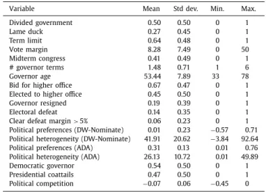
Table A1 Summary statistics.

Variable Mean Std dev. Min. Max.

Divided government 0 .50 0 .50 0 1 Lame duck 0 .27 0 .45 0 1 Term limit 0 .64 0 .48 0 1 Vote margin 8 .28 7 .49 0 50 Midterm congress 0 .41 0 .49 0 1 # governor terms 1 .48 0 .71 1 6 Governor age 53 .44 7 .89 33 78

Bid for higher office 0 .67 0 .47 0 1

Elected to higher office 0 .45 0 .50 0 1

Governor resigned 0 .19 0 .39 0 1

Electoral defeat 0 .14 0 .35 0 1

Clear defeat margin > 5% 0 .06 0 .23 0 1

Political preferences (DW-Nominate) 0 .01 0 .23 −0 .57 0 .71 Political heterogeneity (DW-Nominate) 41 .91 20 .62 −3 .84 92 .64 Political preferences (ADA) 0 .31 0 .13 0 .01 0 .76 Political heterogeneity (ADA) 26 .13 10 .72 0 .01 49 .89

Democratic governor 0 .54 0 .50 0 1 Presidential coattails 0 .47 0 .50 0 1 Political competition −0 .07 0 .06 −0 .45 0 Table A2 Variable descriptions. Variable Description

Dividedgovernment Dividedgovernmentcontrol:1(dividedbranchordividedlegislature),unifiedgovernmentcontrol:0.Mainsource:Altetal.(2006), NationalConferenceofStateLegislators(NCSL)

Lameduck Governorisalameduck:1,0otherwise.Mainsource:ListandSturm(2006),owndatacollectionafter2000 Termlimit Statewithgubernatorialtermlimit:1,0otherwise.Mainsource:ListandSturm(2006),owndatacollectionafter2000 Votemargin Votemarginmeasuredasthepercentagevoteshareofgovernorinvoteoftoptwocandidates-50.Mainsources:ListandSturm

(2006),Leip(2015)

Shortterm(2years) Stateswith2-yeargovernorterms:1,0otherwise(4-yearterms).Mainsource:ListandSturm(2006),owndatacollectionafter2000 Generalelection Generalelectionyear(executiveandlegislative):1,0otherwise.Source.ListandSturm(2006),owndatacollectionafter2000 Midtermcongress Midtermcongress:1,0otherwise.Source:NationalConferenceofStateLegislators(NCSL)

#governorterms Numberofconsecutivegubernatorialterms.Mainsource:Altetal.(2006),owndatacollectionafter2000 Governorage Ageofthegovernor.Source:BesleyandCase(2003),owndatacollection

Bidforhigheroffice Governorrunssubsequentlyforhigherfederaloffice(Senate,HouseofRepresentatives,Presidency).Source:owndatacollection Electedtohigheroffice Governorissubsequentlyelectedtohigherfederaloffice(Senate,HouseofRepresentatives,Presidency).Source:owndatacollection Governorresigned Governordoesnotrunforreelection:1,0otherwise.Source:BesleyandCase(2003),owndatacollection

Governordefeated Governorwasdefeatedinsubsequentelection:1,0otherwise.Source:BesleyandCase(2003),owndatacollection

Politicalpreferences DWNominate:Measureofpoliticalpreferencesonaliberal–conservativescalefromroll-callvotesofmembersofthe94thto111thUS Congress.StatemeanofthefirstdimensionofDW-Nominatescoreofstaterepresentatives(HouseandSenate)inFederalCongress. NegativevaluesforDemocrats,positivevaluesforRepublicans.Source:owncalculationbasedonMcCartyetal.(2006)

AdjustedADAscores:Measureofpoliticalpreferencesonaliberal–conservativescalefromroll-callvotesofmembersofthe94thto 110thUSCongressselectedby“AmericansforDemocraticAction(ADA)”.StatemeanoftheadjustedADAscoreofstate

representatives(HouseandSenate)inFederalCongress(1970–2007).Source:AndersonandHabel(2009)

Politicalheterogeneity DWNominate:StatestandarddeviationofthefirstdimensionofDW-Nominatescoresforstaterepresentatives(HouseandSenate)in theFederalCongress.Source:owncalculationbasedonMcCartyetal.(2006)

AdjustedADAscores:StatestandarddeviationoftheadjustedADAscoreofstaterepresentatives(HouseandSenate)inFederal Congress(1970–2007).Source:AndersonandHabel(2009)

Democraticgovernor Governorisademocrat:1,0otherwise.Mainsource:Besleyetal.(2010),owndatacollectionafter2000 Presidentialcoattail Presidentandgovernorofthesameparty:1,0otherwise.Source:owndatacollection

Politicalcompetition Politicalcompetitionisbasedontheaveragedemocraticvoteshare(d_st )instateexecutiveelectionsandelectionsofUS representatives.κ_st =−|d_st − 0.5|.Source:Besleyetal.(2010)