Optimization of irrigation scheduling for complex water distribution using mixed integer quadratic programming (MIQP)

HAL Id: hal-00783214

https://hal.archives-ouvertes.fr/hal-00783214

Submitted on 31 Jan 2013

HAL is a multi-disciplinary open access

archive for the deposit and dissemination of

sci-entific research documents, whether they are

pub-lished or not. The documents may come from

L’archive ouverte pluridisciplinaire HAL, est

destinée au dépôt et à la diffusion de documents

scientifiques de niveau recherche, publiés ou non,

émanant des établissements d’enseignement et de

Optimization of irrigation scheduling for complex water

distribution using mixed integer quadratic programming

(MIQP)

S. Hong, P.O. Malaterre, Gilles Belaud, C. Dejean

To cite this version:

S. Hong, P.O. Malaterre, Gilles Belaud, C. Dejean. Optimization of irrigation scheduling for complex

water distribution using mixed integer quadratic programming (MIQP). HIC 2012 – 10th International

Conference on Hydroinformatics, Jul 2012, Hamburg, Germany. p. - p. �hal-00783214�

10th International Conference on Hydroinformatics HIC 2012, Hamburg, GERMANY

OPTIMIZATION OF IRRIGATION SCHEDULING FOR COMPLEX

WATER DISTRIBUTION USING MIXED INTEGER QUADRATIC

PROGRAMMING (MIQP)

SOTHEA HONG (1), PIERRE-OLIVIER MALATERRE (1), GILLES BELAUD (2) AND CYRIL DEJEAN (1)

(1) UMR G-Eau, Irstea, 361 rue J.-F. Breton, BP 5095, 34033 Montpellier (2) UMR G-Eau, SupAgro, Place Pierre Viala, 34060 Montpellier, Cedex 02

ABSTRACT

Irrigation scheduling is necessary to ensure the fair water distribution between end-users and to organize gate keepers work. After analyzing water distribution issues at a secondary sector of the Gignac Canal, we developed an approach to optimize water delivery of on-demand distribution policies. MIQP was used to solve such problem. Within irrigation network, water resources and manpower for gate operation constraints, we built an objective function for dual goal: as close as possible to demand load profile and less manpower work. This method will be illustrated for scheduling off-take turnouts of an example chosen from a secondary command area of the Gignac Canal.

INTRODUCTION

In open-channel irrigation networks, the channel is traditionally designed for low volume storage and for agricultural usage only. Water is distributed from the source to outlets based on fixed rotation schedules (seen the definition in Clemmens [3]) which water delivery rarely matches crop needs (Merriam et al. [9]) and leads to water waste. Moreover, increasing of land cultivation and worsening drought conditions have led to the need for water savings. Thus, delivering water to farmer outlets at the right time and in the right quantities is increasingly important (free access). However, the systems are characterized by significant hydraulic constraints, such as time lags and overtopping. Currently, some irrigation schemes have undergone diversification: irrigation techniques, crop patterns and usages (agricultural, urban and industrial usages); e.g., the Gignac Canal scheme in the south of France. These changes generate water distribution complexity. It is actually due to rapidly changing (somehow apparently random) water demands. Satisfactory distribution may be very difficult to achieve. In this situation, on-demand distribution giving farmers the opportunity to present their demands regarding irrigation start time as well as water quantities in advance should be considered. Water delivery through coordinated efforts to manage supply and demand should be optimized.

Optimization of irrigation scheduling has been being studied more than twenty years. The work of Suryavanshi and Reddy [11] is considered as the first optimization approach on the subject by many literature reviews (Wang et al. [13], Anwar et al. [2], de Vrie et al. [4], [5], Wardlaw et al.[14] , Mathur et al. [8], Haq and Anwar [6]). This method was conceived to minimize water flows in the lateral canal by stricter application of the duration

of the irrigation turn. It is called “stream tube method”. The method function was criticized and corrected by Wang et al. [13]. Later, it was improved for optimizing irrigation schedules using arranged-demand by Anwar et al. [2] and De Vries and Anwar [5]. Another technique called “time bloc approach” was developed by Reddy et al. [11] for optimizing the random water demand at the lateral canal level. Recently, the irrigation scheduling using on-demand distribution was developed by Nixon et al. [10] and Li et al. [1]. However, the above techniques are not designed to solve the irrigation scheduling problem linked to flexible decision making on time-on, duration and flow rate, multi-irrigation techniques and priority criteria. To our knowledge, manpower issues associated to gate operations were not mentioned in previous research.

In this paper, optimization of water distribution method using MIQP (Mixed Integer Quadratic Programming) will be described. This approach is based on user water demand parameters: irrigation start time, irrigation duration, and flow rates. These three parameters are considered as input. The decision making process is in accordance with the global solution of the objective function and constraints. The difference between demand and supply should be minimized. Gate operation tasks are also considered in the objective function and constraints in order to optimize the gate keepers work. This method is applied to an example of irrigation scheduling performed in a secondary command area of the Gignac Canal in south of France.

IRRIGATION SCHEDULING OPTIMIZATION USING MIQP

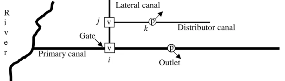
In most cases, water is diverted from sources such as rivers or reservoirs by a main canal at fairly stable flow rates to irrigation schemes. Lateral or secondary canals are connected to the main canal and supply several distribution areas. The water turn is generally performed at this level. Some outlet groups need a distributor or tertiary canal to transfer water from the lateral canal as seen in Figure 1. Water delivery from the canal to sub canal is controlled by means of a manually–operated gate. The farm outlets can be connected to any hierarchical level of canal. Otherwise, each outlet follows the indices i, j and k which represent the off-takes on the main canal, the lateral canal and the distributor canal respectively.

For on-demand scheduling, each outlet is characterized by three demand parameters: 1) irrigation start time (td ), 2) duration ( dd ) and 3) flow rate ( qd ). The issue that must be

Figure 1: Irrigation scheme1 Gate Primary canal R i v e r Distributor canal Lateral canal j k i _Outlet p p v v

addressed is how to set optimal supply levels that take into account these three random demand variables while satisfying all actors (users and irrigation manager).

Objective function

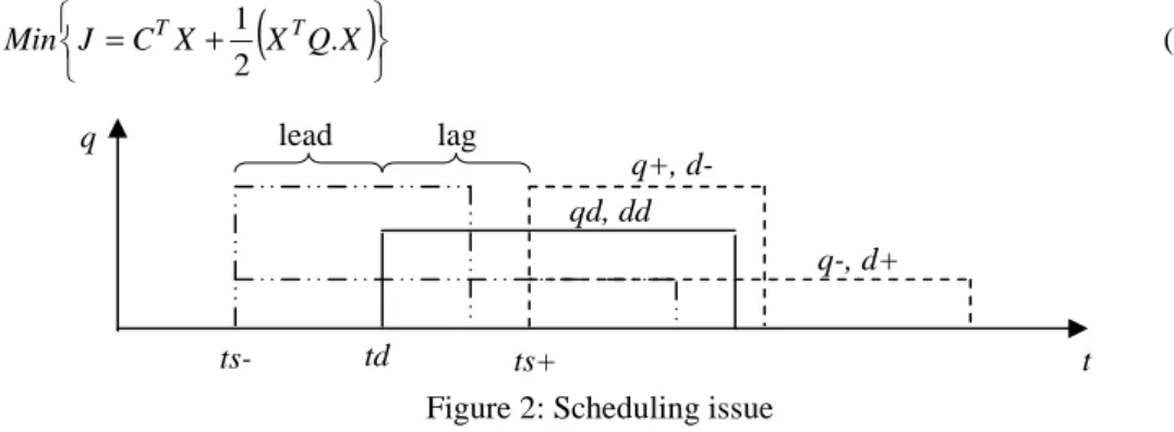
For on-demand scheduling, the objective is to deliver water to users as close as possible to their requests. Therefore, the deviation between demand and supply should be minimized. The deviation of irrigation start time, irrigation duration, and flow rate as well as water quantity are considered. Concerning irrigation start time, it can be at any time (lead

ts

−, lag

ts

+ or right timetd ) in accordance with global distribution resolution. Similarly,

irrigation duration and flow rate can be equal (dd ,qd), inferior (d ,− q−) or superior (d ,+ q+) to demand (Figure 2). Whereas, water quantity supply must be equal or inferior to demand. The quantity parameter is used to make a decision on duration and flow rates which should be adjusted in opposite directions (Figure 2); e.g., when irrigation duration increases, water flow should be decreased. In this paper, all deviation comparing to the request were taken into account as penalty costs. We use a quadratic function to develop our approach. And three decision variables 1) start time (ts), 2) irrigation duration (d) and 3) water flow (qs ) are integer numbers.

As described above, irrigation techniques and crop patterns have been diversified. Water should be diverted to outlets based on priority criteria. We propose three priority coefficients linked to start time (cts), flow rate (cqs) and volume (cqv). Furthermore, water

distribution is a complex task. Water is diverted from the sources to end-users through hydraulic structures and the delivery is controlled by means of gates which are generally manually operated (the approach would be the same if the regulating structures were weirs). To carry out the distribution and to reduce operation cost, their tasks should also be minimized. The duration of one job depends on the distance of the operation site from where the previous job was performed. Nevertheless, to simplify the duration determination for each job, we use the maximum job duration for all jobs. Thus, the number of jobs possible for gate keepers during irrigation schedule is defined as the maximum number (Mo_max) which we should try to reduce. Mo_max for each work period is the result of division between the duration of work period and the maximum job duration. We use a Boolean variable (

mo

) to define a gate operation. This variable is nil when the operation is not required and one otherwise. Therefore, the objective function can be written as follows:

(

)

₁23 4 5 6 + =C X X QX J Min T T . 2 1 (1)

Figure 2: Scheduling issue

qd, dd q+, d- q-, d+ td ts- ts+ t lag lead q

Where Cand Q are matrix coefficients of the objective function cost. Their sizes depend on the size of the X state vector variables.

NN ijk ijk ijk N tijk tijk ijk ijk ijk ijk ijk ijk N tijk tv tv tijk ijk ijk ijk Q and w qd dd td C y qp mo q qs d ts X 77 7 7 7 7 7 7 7 7 8 9 AA A A A A A A A A B C = 77 7 7 7 7 7 7 7 7 7 8 9 AA A A A A A A A A A B C − − − = 77 7 7 7 7 7 7 7 7 7 8 9 AA A A A A A A A A A B C = 0 . . . . . 0 . . . . . . . . . . . . . . . . . . 0 . . . . . . 2 0 . . . . . 0 2 0 0 . . . . 0 2 0 ) ( 2 ) ( 2 ) ( 2 , 6 ϕ β α γ φ ϕ β α Where

D

DDD

DDD

DDD

DDD

= = = = = = = = = = = = = = ∆ = ∆ = ∆ = ∆ = int 1 int int max 5 1 1 1 2 max 4 1 1 1 2 max 3 1 1 1 2 max 2 1 1 1 2 max 1 ) ( and ) ( ) ( ) ( ) ( , ) ( , ) ( ) ( nb n i mi j pij k ijk qv ijk n i mi j pij k ijk qs ijk n i mi j pij k ijk n i mi j pij k ijk ts ijk Mo w qv c w q c w d w t c w γ φ ϕ β α

and i,jandk are the outlet indices, t is the time index and v is the gate index. In the X variable, the three additional variables are defined for 1) the outlet flow rate as a function of time (q), 2) the unused water flow at each canal exit (qp) and 3) the outlet irrigation time (y). The variables q and qp are integer variables and y is a Boolean variable. y is equal to one during the irrigation time associated with each outlet, and to zero the rest of the time. Each term value in the objective function should be between 0 and 1. In fact, the sum of the difference between supply and demand squared is divided by the sum of the maximum deviation squared. ∆t_max,∆d_max,∆q_maxand∆qv_maxare maximum deviation of start time, duration, flow rate and volume respectively. Furthermore, we also introduce penalty factor costs (wf=1→6) to the above terms thereby providing more options to irrigation policies.

Constraints

To ensure distribution and to obtain fair irrigation performance, every water turn should respect some constraints. The first one is that all individual water turns should be completed before the end of the schedule period (T).

T d

tsijk+ ijk ≤ (2)

As y is a Boolean variable and represents the irrigation time, and M is as high a positive value as required to respect the conditions below, we can write the constraint to determine y for each job or outlet as follows:

E E E 4 E E E 5 6 ∀ + ≥ − + + ∀ ≤ − − ∀ = +

D

= k j i t t y M d ts k j i t t y M ts k j i y d tijk ijk ijk tijk ijk T t tijk ijk and , , 1 ) 1 ( and , , ) 1 ( and , 0 1 (3)

Where t is defined for the time horizon (time slots). In order to avoid perturbation during the irrigation period, the water flow for each outlet should be constant. Thus, while

y is equal to one, the variable

q

is equivalent to

qs

.

E E 4 EE 5 6 ∀ ≤ − ∀ ≤ − ∀ ≥ − + − k j i t My q k j i t qs q k j i t y M qs q tijk tijk ijk tijk tijk ijk tijk and , , 0 and , , 0 and , , 0 ) 1 ( (4)

All modifications of the water position are considered as operations. The constraints below are used to count the number of operations for each gate. n,miandpij are the maximum values of i,jandk indices. mi depends on iand pij on i and . j

(

)

(

)

(

)

(

)

E E E E E 4 E E E E E 5 6 ≥ ∀ ≤ − + − − ≥ ∀ ≥ − + + − = ∀ ≤ − = ≤ −

DDD

DDD

DDD

DDD

DDD

= = = = = = − − = = = = = = − − = = = n i mi j pij k v t tv tv n i mi j pij k ijk t tijk n i mi j pij k v t tv tv n i mi j pij k ijk t tijk v v n i mi j pij k v ijk v t qp qp mo M q q v t qp qp mo M q q t mo M qp t mo M q 1 1 1 ) 1 ( 1 1 1 ) 1 ( 1 1 1 ) 1 ( 1 1 1 ) 1 ( 1 1 1 1 1 1 1 and 2 , 0 and 2 , 0 1 , 0 1 , 0 (5)

The variable mo can be equal to one only for the work period of gate keepers and to zero outside of this period. tmosandtmof are the gate keepers’ work start time and end time respectively. nbintis equal to the number of work periods.

E E E 4 E E E 5 6 ≤ ≥ ∀ ≥ − + ≤ ≤ ∨ − ≤ ∀ ≤ − −

D D

+∆ = = − t t t t nb v tv nb tv nb t t tv van mo tmof t t mo M tmof tmos t tmof tmos t t mo M tmos 1 ) 1 ( 1 int 1 ) 1 ( 1 ) 1 ( int int (6)

As water saving is increasingly a hot topic, the supply of water volume that is superior to the demand is seen as very wasteful. In this context, water supply must match or be inferior to the demand volume. However, it should also respect the minimum supply level.

t

δ is the time slot for our simulation.

E E 4 E E 5 6 ∀ ≥ ∀ ≤

D

D

= = T t ijk l tijk T t ijk tijk k et j i qvd qv t q k et j i qvd t q 1 min 1 δ δ (7)

On the other hand, all decisions on outlet flow rates must take into account the available flow rate (Qr) as well as the volume. nbc is the number canal.

DDD

D

= = = = ∀ ≤ + n i mi j pij k t nb v tv tijk qp Qr t q v 1 1 1 1 (8) Besides that, irrigation network capacities are limited to distribute water to all users simultaneously. We put some more constraints to primary flow rate capacity. The canal is

Figure 3: Example of irrigation network

generally divided into pools which have their own capacity (Qc_pool). ipool is the initial

number and npool the maximum value of

i

at each pool. To lateral canal and distributor, its actual flow rate must be inferior or equal to its capacity (Qc_iandQc_ij).

n npool ipool and t Qc q npool ipool i mi j pij k pool tijk ≤ ∀ ≤ ≤ ≤

D D D

= =1 =1 1 (9)

DD

= = ≥ ∀ ≤ mi j pij k i tijk Qc i mi t q 1 1 and ) 2 ( (10)

D

= ≥ ∀ ≤ pij k ij tijk Qc ietj pij t q 1 and ) 2 ( (11) APPLICATION

The method is applied to a command area of a secondary irrigation canal of the Gignac Canal for scheduling water user demands. This sector has about 130 ha of irrigated land, mainly vineyards. Nowadays, this command area is in the complex situation of diversified crop pattern, mixed usages (farming and urban), different irrigation techniques and mixed distribution scheduling (rigid rotation and arranged schedule). In addition, it faces water scarcity in June and July and less water turn respect (after analyzing data collected in summer 2010). This sector has 201 outlets including 9 urban outlets.

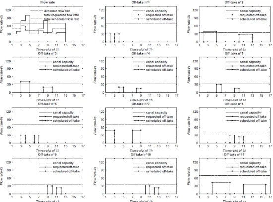
Here, we studied the irrigation scheduling of a network example with 11 outlets extracted from the studied sector for a 12 h period. The irrigation starts at 8 h and finishes at 20 h. In this example, two gates are operated manually by gate keepers at two intervention periods: 1) from 8 to 9 h, and 2) from 11 to 13 h. The requested load profiles are presented in Figure 4. For all outlets, we consider the same priority criteria. The flow rate at lateral canal inlets matches 70 l/s during 12 h for supplying 11 outlets downstream through a lateral canal (capacity of 70 l/s), two other distributor’s canal and two of their sub canals that have the same capacity of 35 l/s.

Equations (1) to (11) were transformed into matrix formulation within Matlab software. The IBM-Ilog Cplex solver is called to find an optimum solution. For 11 outlets during 12 h which was set to 13 time slots of 1 h, the problem has 371 variables and 923 constraints to be solved. The result of the optimization is shown in the graphs of Figure 4. The objective function cost was found to be 0.235 (by considering wf=1/6). The total water

taken from the canal was found to be inferior to the available amount (ratio = 60%). However the adequacy (using Gates et al [7]’s method) on water quantity was estimated to

Lateral canal inlet

1 5 3 4 6 7 10 8 9 11 v v 2

Figure 4 : Requested and scheduled load profiles

be 79%, i.e. the scheduled volume was inferior to the requested ones by 21%. Actually, it is caused by the canal capacity and manpower constraints. The work of the gate keepers was reduced from 8 (maximum work) to 2 (optimum work). Moreover, the adequacy on start time was found to be 36% early and 20% late compared to demands. While, we found the adequacy 98% on demanded irrigation duration and 81% on demanded flow rate.

CONCLUSIONS

This paper introduces a new method for irrigation scheduling using on-demand distribution policies. The technique proposed uses MIQP algorithm which objective function was developed based on a quadratic function. We proposed six terms for this function, with four being defined for user adequacy, one for water distribution cost linked to gate operation and the last one concerns water lost. First, this optimization procedure allows a flexible decision making on irrigation start time, irrigation duration and outlet flow rate, as close as possible to the requested load profile. Second, it enables taking into account priority criteria referring to crop pattern, irrigation technique, usage type, and outlet location. Moreover, it can optimize the gate operation.

However, water delivery needs transit time which depends on the hydraulic state of the canals. We will take this into account in future work. The present work also assumes that

gate operation duration is constant for all operation jobs. Nevertheless, it can be variable depending on the distance between the gates. Also, it may be better to minimize the distance covered by the gate keeper instead of the number of operations. Finally, standard water demand, weather prediction and previous irrigations should be considered as closed loop calculation.

REFERENCES

[1] Alende J., Li Y. and Cantoni M., “A 0,1 linear program for fixed-profile load scheduling and demand management in automated irrigation channels”, 48th IEEE Conference on Decision and Control held jointly with 2009 28th Chinese Control Conference, CDC/CCC 2009, 2009, 597-602 .

[2] Anwar A. and Clarke D., “Irrigation scheduling using mixed-integer linear programming”, J. Irrig. Drain. Eng., 127, 2001, 63-69.

[3] Clemmens A., “Planning Operation Rehabilitation and Automation of Irrigation Water Delivery Systems”, ASCE, 1987

[4] De vries T. and Anwar A., “Irrigation scheduling with travel times”, J. Irrig. Drain. Eng., 132, 2006, 220-227

[5] De vries T. and Anwar A., “Irrigation scheduling. I: Integer programming approach”, J. Irrig. Drain. Eng., 130, 2004, 9-16

[6] Haq Z. and Anwar A., “Irrigation scheduling with genetic algorithms”, J. Irrig. Drain. Eng., 136, 2010, 704-714

[7] Gates T. K., Heyder W. E., Fontane D. G. and Salas J. D., “Multicriterion strategic planning for improved irrigation delivery. I: Approach”, J Irrig Drain Eng, 117, 1991, 897-913

[8] Mathur Y. P., Gunwant S. and Pawde A. W., “Optimal Operation Scheduling of Irrigation Canals Using Genetic Algorithm”, International Journal of Recent Trends in Engineering, 1, 2009, 11-15

[9] Merriam J., Styles S. and Freeman B., “Flexible irrigation systems: Concept, design, and application”, J. Irrig. Drain. Eng., 133, 2007, 2-11

[10] Nixon J. B., Dandy G. C. and Simpson A. R., “A genetic algorithm for optimizing off-farm irrigation scheduling”, Journal of Hydroinformatics, 3, 2001, 11-22

[11] Reddy J., Wilamowski B. and Cassel-Sharmasarkar F., “Optimal scheduling of irrigation for lateral canals, International Journal of Recent Trends in Engineering”, 48, 1999, 1-12

[12] Suryavanshi A. and Reddy J., “Optimal operation schedule of irrigation distribution systems”, Agricultural Water Management, 11, 1986, 23 - 30

[13] Wang Z. Reddy, J. & Feyen, J. , Improved 0-1 programming model for optimal flow scheduling in irrigation canals, Irrig Drainage Syst, Kluwer Academic Publishers, 1995, 9, 105-116

[14] Wardlaw, R., and Bhaktikul K., “Comparison of genetic algorithm and linear programming approaches for lateral canal scheduling”, J. Irrig. Drain. Eng., 130, 2004, 311-317