HAL Id: hal-00296995
https://hal.archives-ouvertes.fr/hal-00296995
Submitted on 16 May 2007
HAL is a multi-disciplinary open access
archive for the deposit and dissemination of
sci-entific research documents, whether they are
pub-lished or not. The documents may come from
teaching and research institutions in France or
abroad, or from public or private research centers.
L’archive ouverte pluridisciplinaire HAL, est
destinée au dépôt et à la diffusion de documents
scientifiques de niveau recherche, publiés ou non,
émanant des établissements d’enseignement et de
recherche français ou étrangers, des laboratoires
publics ou privés.
Comparison of different approaches to quantify the
reliability of hydrological simulations
C. Gattke, A. Schumann
To cite this version:
C. Gattke, A. Schumann. Comparison of different approaches to quantify the reliability of
hydro-logical simulations. Advances in Geosciences, European Geosciences Union, 2007, 11, pp.15-20.
�hal-00296995�
www.adv-geosci.net/11/15/2007/ © Author(s) 2007. This work is licensed under a Creative Commons License.
Geosciences
Comparison of different approaches to quantify the reliability of
hydrological simulations
C. Gattke and A. Schumann
Ruhr-University Bochum, Institute of Hydrology, Water Resources Management and Environmental Engineering, Bochum, Germany
Received: 17 January 2007 – Revised: 11 April 2007 – Accepted: 4 May 2007 – Published: 16 May 2007
Abstract. The focus of this study was to compare
differ-ent uncertainty estimation approaches to evaluate their abil-ity to predict the total amount of uncertainty in hydrologi-cal model predictions. Three different approaches have been compared. Two of them were based on Monte-Carlo sam-pling and the third approach was based on fitting a prob-ability model to the error series of an optimized simula-tion. These approaches have been applied to a lumped and a semi-distributed model variant, to investigate the effects of changes in the model structure on the uncertainty assess-ment. The probability model was not able to predict the total amount of uncertainty when compared with the Monte-Carlo based approaches. The uncertainty related to the simulation of flood events was systematically underestimated.
1 Introduction
Hydrological models are common tools for water resources planning and management. They are used to e.g. predict wa-ter balances or extreme events (floods and droughts), to ex-trapolate discharge time-series or to evaluate management strategies. Despite the efforts devoted to model develop-ment within the past decades, there is still significant un-certainty associated with hydrological simulations (Monta-nari and Brath, 2004). This applies to both conceptual and physically based models. The uncertainty in hydrological model output stems from three main causes: (i) the model un-certainty, which denotes incompatibilities between the struc-tures represented in the model and the strucstruc-tures present in the hydrological system, (ii) the parameter uncertainty and (iii) the data uncertainty, which applies to the input data (e.g. precipitation and temperature) as well as to the data used for calibration (e.g. discharge). Recognizing the problem of
un-Correspondence to: C. Gattke
(christian.gattke@rub.de)
certainty, many different approaches to quantify the reliabil-ity of hydrological simulations have been proposed in recent years (Montanari and Brath, 2004).
Conventional “point” methods, such as first-order analy-sis, calculate the mean and variance of the predicted variable, based on the mean and variance of uncertain inputs and/or parameters. They rely on the assumption that a single lin-earization of the system performance function at the central values of the basic variables is representative of the statistical properties of system performance over the complete range of basic variables (Melching, 1995). These point-estimation methods are limited by the assumption of approximate lin-earity of the model (Gupta et al., 2005), which is often not suitable for hydrological models. Due to this problem, sim-ulation based approaches that explore the feasible parame-ter space and/or consider an uncertainty range for the data sets are commonly used for uncertainty assessment nowa-days. The most used simulation based approach for inferring the global simulation uncertainty is probably the Generalized Likelihood Uncertainty Estimation (GLUE) method (Beven and Binley, 1992). A third option to estimate the simula-tion uncertainty is to analyze the statistical properties of the model error series that occurred in reproducing observed dis-charge data. An example for such an approach is the Meta-Gaussian model, recently presented by Montanari and Brath (2004).
However, only few studies compare different uncertainty estimation approaches (e.g. Montanari and Brath, 2004; McIntyre et al., 2002) to evaluate their ability to predict the total amount of uncertainty in hydrological model predic-tions. The goal of the study presented here was to carry out such a comparison between three different approaches (two simulation-based and a stochastic error model). The three uncertainty estimation approaches have been applied to two model variants with different spatial discretizations to inves-tigate the effects of changes in the model structure on the uncertainty assessment.
16 C. Gattke and A. Schumann: Reliability of hydrological simulations
2 Model structures and data
The two model variants used in this study where imple-mented following the concept of the HBV-96 model (Lind-str¨om et al., 1997). One significant difference lies in the gen-eration of surface runoff. Within the original HBV model all water from the soil routine that does not evaporate recharges
into the upper response box. In contrast to this, for the
model applications presented here, surface runoff can occur from saturation excess and is routed to the stream network via simple linear storage. The triangular weighting func-tion to smooth the generated discharge has been excluded, owing to daily time step discretization and detailed struc-turing of the area under investigation into subbasins. The Muskingum method was used for the flood routing within the river reaches. The first model variant used lumped repre-sentations of all vertical model components within the sub-basins. The second model variant used semi-distributed rep-resentations of the interception layer (depending on land use distribution), the root zone layer (combination of land use and soil types) and the upper response layer (distribution of soil types). The recession constants of the upper response boxes were scaled depending on transmissivity and average distance to the stream network. Implementation of both vari-ants was based on an object-oriented framework designed for adaptive development of hydrological models (Gattke and Pahlow, 2006). The study was carried out for a mesoscale catchment located at the upper Werra river in Mid-East
Ger-many (Meiningen, 1167 km2). The catchment was divided
into 39 subbasins. A six-year period (Nov 1991–Oct 1997) of observed discharge and meteorological data was available. The issue of appropriate data lengths for model identification has been investigated by a variety of studies, the general re-sult being that the required length mainly depends on data quality, model complexity and climatic variability (Wagener and McIntyre, 2005). Considering the results of Wagener and McIntyre who used a three-year calibration period to com-pare different objective functions, the six-year period used here was deemed to be adequate. The simulations were car-ried out at a daily time-step. The maximum peak discharge observed in this period was 181 m3/s (April 1994). The av-erage discharge was 14.5 m3/s. The average annual precipi-tation depth over the basin area was 838 mm/yr.
3 Uncertainty assessment
Three different uncertainty estimation approaches (two simulation-based and a stochastic error model) were used in this study: a) 0.05- and 0.95-quantiles of the simulated discharge values, b) the quantiles estimated with the GLUE likelihood-weighting procedure and c) the confidence inter-vals obtained by application of the Meta-Gaussian model of Montanari and Brath (2004). Montanari and Brath presented an approach to estimate the uncertainty of a calibrated
hydro-logical model. They make use of a Meta-Gaussian model in order to estimate the probability distribution of the model er-ror conditioned by the simulated discharge. Model residues and model simulations are considered as realisations of two stochastic processes. The standard normal quantile transform (NQT) is used to make the marginal probability distributions of both Gaussian. The normalised series are assumed to be stationary and ergodic. This approach can be applied to mod-els with a varying complexity. Rejecting the concept of an optimum parameter set, Beven and Binley (1992) developed their generalized likelihood uncertainty estimation (GLUE) method. First, a large number of parameter sets is gener-ated randomly via sampling from assumed prior parameter distributions (usually uniform). After performing the simu-lation trials the parameter sets are weighted with an arbitrary chosen goodness-of-fit criterion (likelihood measure). This criterion is employed to differentiate behavioural and non-behavioural parameter sets and to reject the latter ones. The likelihood weights of the accepted parameter combinations are rescaled to produce a cumulative sum of one and used to construct a cumulative distribution function of the simu-lated discharge values. This allows uncertainty bounds to be derived at every time step.
Both the GLUE approach and the Meta-Gaussian model are supposed to consider all sources of uncertainty implic-itly. In case of the GLUE procedure this occurs through the likelihood weighting (Beven and Freer, 2001). To verify this assumption the 0.05- and 0.95-quantiles of the simulated dis-charge values were also included in the comparison shown here. The Nash-Sutcliffe efficiency (NSE) was used as like-lihood measure (Nash and Sutcliffe, 1970). The rejection criterion shows considerable effects on the simulation range and therefore on the possibility that observed values are lying outside of this range (Montanari, 2005). Thus this criterion should be chosen carefully on the one hand to avoid a simu-lation range too narrow and on the other hand to avoid blur-ring of the models predictive performance by an extremely wide simulation range. Here the 3rd quartile of the simu-lations has been used as rejection criterion. In total, 10 000 simulations with parameter sets obtained by randomly gener-ated, uniformly distributed values were performed with both model variants (lumped and semi-distributed). The simula-tions with the maximum NSE values were selected to esti-mate the model uncertainty by means of the Meta-Gaussian approach.
4 Results
The results obtained for the maximum NSE and the 3rd quar-tile values were 0.905 and 0.787 for the lumped model vari-ant and 0.919 and 0.792 for the semi-distributed varivari-ant re-spectively. Hence simulation runs with NSE less than 0.787 (lumped) and 0.792 (semi-distributed) had been rejected.
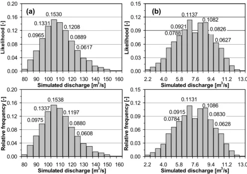
0.1530 0.0965 0.1331 0.1208 0.0889 0.0617 0.00 0.04 0.08 0.12 0.16 0.20 80 90 100 110 120 130 140 150 160 Simulated discharge [m3/s] L ik e li h o o d [-] 0.1137 0.0627 0.0826 0.1082 0.0921 0.0788 0.00 0.03 0.06 0.09 0.12 0.15 2.2 4.0 5.8 7.6 9.4 11.2 13.0 Simulated discharge [m3/s] L ik e li h o o d [-] 0.1131 0.0915 0.0784 0.1086 0.0628 0.0830 0.00 0.03 0.06 0.09 0.12 0.15 2.2 4.0 5.8 7.6 9.4 11.2 13.0 Simulated discharge [m3/s] R e la ti v e fr e q u e n c y [-] 0.1538 0.1337 0.1197 0.0975 0.0880 0.0608 0.00 0.04 0.08 0.12 0.16 0.20 80 90 100 110 120 130 140 150 160 Simulated discharge [m3/s] R e la ti v e fr e q u e n c y [-] (a) (b)
Fig. 1. Posterior distribution of the GLUE likelihood weighted model predictions (top) and the relative frequency of the simulated discharge
values (bottom), (a) extreme winter flood (30 Jan 1995), (b) single daily discharge value out of a low-flow period during summer (12 Aug 1995).
4.1 Comparison of the simulation-based prediction ranges
The comparison of the prediction quantiles estimated with GLUE and the quantiles of the simulated discharge values confirmed, as expected, that these are not identical, i.e. the 90% GLUE prediction limits do not comprise 90% of the simulated discharge values. Overall the differences between both quantile ranges were negligible. The average absolute difference of the compared prediction limits over the entire simulation period of six years was less than 0.03 m3/s for both model variants. This corresponds to a difference of 0.1% for the upper and lower limit. This consistency arises from the fact that the posterior distribution of the likelihood weighted model predictions, as derived from the GLUE pro-cedure and the relative frequency of the simulated discharge values, are in good agreement. Figure 1 exemplifies this for two simulation time steps with different flow magnitudes. Shown are the peak of an extreme winter flood (30 Jan 1995, Fig. 1a) and a single daily discharge value out of a low-flow period during summer (12 Aug 1995, Fig. 1b). Fur-thermore, this example confirms that the distributions have characteristics with changing shape and variance over time
as demonstrated by Beven and Freer (2001). The
distri-butions are clearly non-Gaussian for the peak-flow. More substantial differences between the prediction ranges do not occur until 90% of all simulations out of the Monte-Carlo sample (this corresponds to a threshold of about 0.3 for the NSE) are accepted as behavioural and are included in the un-certainty analysis. However, this would be an implausible
Table 1. Average uncertainty ranges (in m3/s) over the six-year pe-riod for different magnitude classes of the observed discharge (MQ
= average discharge = 14.5 m3/s).
Model structure Lumped Semi-distributed Approach GLUE Meta-Gauss GLUE Meta-Gauss Overall 9.5 12.9 10.0 11.6
>3 MQ 44.4 21.6 40.8 28.4
<MQ 6.1 15.0 6.6 13.4
choice. Thus, further discussion is restricted to the compar-ison of the GLUE method and the Meta-Gaussian model of Montanari and Brath (2004).
4.2 Comparison of simulation-based prediction ranges and
the confidence intervals estimated with the Meta-Gaussian Model
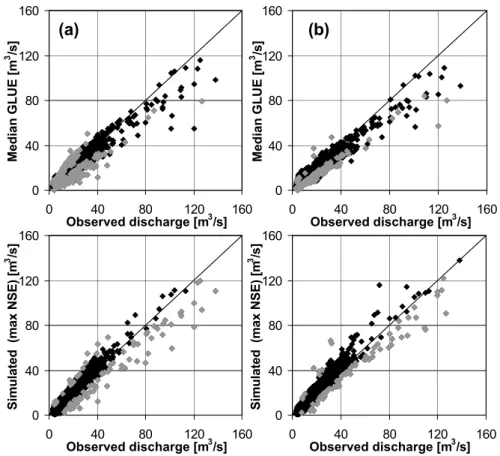
Figure 2 compares the observed discharge values over the six-year period that lie outside the different uncertainty ranges for both model variants. The Median GLUE output has been chosen as a representative for the simulation range. In both cases the observed discharge was systematically un-derestimated in the high flow regime by the Median GLUE. This is due to skewness of the GLUE simulation range at time steps with high-flows, as shown in the previous section. For
18 C. Gattke and A. Schumann: Reliability of hydrological simulations 0 40 80 120 160 0 40 80 120 160 Observed discharge [m3/s] Me d ia n G L U E [m 3 /s ] 0 40 80 120 160 0 40 80 120 160 Observed discharge [m3/s] Me d ia n G L U E [m 3 /s ] 0 40 80 120 160 0 40 80 120 160 Observed discharge [m3/s] Si m u la te d (m a x N SE) [m 3 /s ] 0 40 80 120 160 0 40 80 120 160 Observed discharge [m3/s] Si m u la te d (m a x N SE) [m 3 /s ]
(a)
(b)
Fig. 2. Dotty plots of Median GLUE vs observed discharge (top) and simulated vs observed discharge (bottom) for the six-year period. Grey
dots indicate observed discharge values lying outside the uncertainty ranges of GLUE (top): (a) lumped model variant (18.8% of overall values, 12.5% of values >3 MQ), (b) semi-distributed model variant (16.1%, 12.5%) and the Meta-Gaussian model (bottom): (a) lumped model variant (4.6%, 46.6%), (b) semi-distributed model variant (3.8%, 42.0%).
the lumped model 18.8% of the overall observed discharge values and 12.5% of the high-flow values (>3 times of aver-age discharge MQ) were lying outside the 90% GLUE simu-lation range (see Fig. 2a, top). The model performs with low-est accuracy for the low-flows and smaller flow peaks during the summer period, which are mostly underestimated. This can be interpreted as a systematic underestimation of the soil moisture dynamics for dry conditions due to lumped model representation of the runoff generating processes. Applica-tion of the semi-distributed structure resulted in better model performance, illustrated by the reduced scatter in the mid-and low-flow region (see Fig. 2b, top). Thus, the percentage of observed values lying outside the prediction ranges was reduced to 16.1, while the percentage of the high-flow values remained unchanged.
The analysis of the uncertainty ranges estimated with the Meta-Gaussian model leads to different results. The amount of observed values lying outside the uncertainty ranges re-duces to 4.6% (lumped) and 3.8% (semi-distributed). On the other hand, the amount of high-flow values lying outside is increased to 46.6% and 42.0% respectively (see Fig. 2a and b, bottom). This is due to opposite trends regarding the
quan-tification of the uncertainty for different regions of the flow regime. Table 1 summarizes the average uncertainty ranges estimated for different magnitude classes of the observed dis-charge. The uncertainty in the low-flow regions (observed values smaller than average discharge MQ) estimated by the Meta-Gaussian model is about two times higher than the un-certainty obtained with the GLUE approach. The situation is approximately reversed for the high flows (observed values
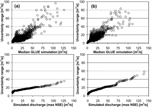
>3 MQ). Figure 3 compares the dependency of the
uncer-tainty range on the magnitude of the simulated discharge. In case of the Meta-Gaussian model the basic hypothesis that the cross dependence between the simulated discharge and the model error is governed by a normal linear equation leads to a monotonically increasing relation. In contrast to this, the relationships for uncertainty ranges estimated with GLUE exhibit an increasing trend, but this is connected with con-siderable scatter. This may be due to different hydrological situations (e.g. ascent or recession period of the hydrograph, influence of snowmelt etc.).
Figures 4 and 5 compare the uncertainty ranges for one year out of the six-year period. Due to the moderate per-formance of the lumped model in the summer period (the
0 20 40 60 80 100 0 25 50 75 100 125 150
Simulated discharge (max NSE) [m3/s]
U n c e rta in ty r a n g e [m 3 /s ] 0 20 40 60 80 100 0 25 50 75 100 125 150
Median GLUE simulation [m3/s]
U n c e rta in ty r a n g e [m 3 /s ] 0 20 40 60 80 100 0 25 50 75 100 125 150
Simulated discharge (max NSE) [m3/s]
U n c e rta in ty r a n g e [m 3 /s ] 0 20 40 60 80 100 0 25 50 75 100 125 150
Median GLUE simulation [m3/s]
U n c e rta in ty r a n g e [m 3 /s ] (a) (b)
Fig. 3. Dependency of the uncertainty ranges of GLUE (top) and the Meta-Gaussian model (bottom) on the magnitude of the simulated
discharge, (a) lumped model variant, (b) semi-distributed model variant.
0 30 60 90 120 150 180 11.94 01.95 03.95 05.95 07.95 09.95 Date Q [m 3/s ] 0 30 60 90 120 150 180 P [m m /d ] Meta-Gauss Precipitation GLUE Observed
Fig. 4. Comparison of the uncertainty ranges for one year out of the
six-year period (lumped model variant).
small flow fluctuations cannot be reproduced, as indicated by the GLUE prediction ranges) the Meta-Gaussian model tends to overestimate the uncertainty, compared to the results ob-tained with GLUE. On the other hand the uncertainty ranges show stronger conformity for the semi-distributed model. However, the uncertainty connected with the simulation of the extreme winter event seems to be underestimated in both cases by the Meta-Gaussian model.
0 30 60 90 120 150 180 11.94 01.95 03.95 05.95 07.95 09.95 Date Q [m 3/s ] 0 30 60 90 120 150 180 P [m m /d ] Meta-Gauss Precipitation GLUE Observed
Fig. 5. Comparison of the uncertainty ranges for one year out of the
six-year period (semi-distributed model variant).
5 Conclusions
The main objective of the study presented here was to com-pare different uncertainty estimation approaches to evaluate their ability to predict the total amount of uncertainty in
hy-drological model predictions. Three different approaches
have been compared. Two of them were based on Monte-Carlo sampling and the third approach was based on fitting a probability model to the error series of an optimized simula-tion (i.e. the one with the best model performance out of the Monte-Carlo sample). These approaches have been applied to a lumped and a semi-distributed model variant, to inves-tigate the effects of changes in the model structure on the
20 C. Gattke and A. Schumann: Reliability of hydrological simulations uncertainty assessment. The 0.05- and 0.95-quantiles of the
simulated discharge values and the corresponding quantiles estimated with the GLUE likelihood-weighting procedure exhibited only negligible differences. This result may re-quire verification, e.g. the application of different likelihoods measures (including real likelihood functions) and/or differ-ent model structures. However, experimdiffer-ents that included more simulations from the Monte-Carlo sample for the un-certainty assessment suggested, that the likelihood weight-ing leads to a smoothweight-ing of the predicted uncertainty range. Thus, the assumption that the GLUE approach handles im-plicitly any effects of errors in the model structure and the data appears questionable. Particularly the latter may re-quire explicit consideration, e.g. by application of a range (or different realizations) of the input data (e.g. Haberlandt and Gattke, 2004). The Meta-Gaussian model was not able to predict the total amount of uncertainty when compared with the GLUE approach. The uncertainty related to the simula-tion of flood events was systematically underestimated. On the other hand, the different estimation of uncertainty in the summer period for both model variants (lumped and semi-distributed) strongly indicated a structural inadequacy of the lumped model. However, the quantity of the difference was not justified by the GLUE approach.
Edited by: K.-E. Lindenschmidt Reviewed by: Y. Wang and T. Weichel
References
Beven, K. and Binley, A.: The future of distributed models: model calibration and uncertainty prediction, Hydrol. Processes, 6, 279–298, 1992.
Gattke, C. and Pahlow, M.: Using object oriented methods for adap-tive hydrological model development and uncertainty estimation, in: Proceedings of the 7th International Conference on Hydroin-formatics, edited by: Gourbesville, P., Cunge, J., Guinot, V., and Liong, S.-Y., 2, 1317–1324, 2006.
Gupta, H. V., Beven, K. J., and Wagener, T.: Model calibration and uncertainty estimation, in: Encyclopedia of hydrological sci-ences, edited by: Anderson, M. G. and McDonnell, J. J., et al., John Wiley & Sons Ltd., Chichester, 2005.
Haberlandt, U. and Gattke, C.: Spatial interpolation vs. simulation of precipitation for rainfall-runoff modelling – a case study in the Lippe river basin, in: Hydrology: Science and practice for the 21st century, edited by: Webb, B., Acreman, M., Maksimovic, C., Smithers, H., and Kirby, C., Proceedings of the British Hy-drological Society International Conference, 1, 120–127, 2004. Lindstr¨om, G., Johansson, B., Persson, M., Gardelin, M., and
Bergstr¨om, S.: Development and test of the distributed HBV-96 model, J. Hydrol., 201, 272–288, 1997.
McIntyre, N., Wheater, H., and Lees, M.: Estimation and propaga-tion of parametric uncertainty in environmental models, J. Hy-droinformatics, 4(3), 177–198, 2002.
Melching, C. S.: Reliability estimation, in: Computer models of watershed hydrology, edited by: Singh, V., Water Resources Pub-lications, 69–118, 1995.
Montanari, A.: Large sample behaviors of the generalized like-lihood uncertainty estimation (GLUE) in assessing the uncer-tainty of rainfall-runoff simulations, Water Resour. Res., 41(8), W08406, doi:10.1029/2004WR003826, 2005.
Montanari, A. and Brath, A.: A stochastic approach for assess-ing the uncertainty of rainfall-runoff simulations, Water Resour. Res., 40(1), W01106, doi:10.1029/2003WR002540, 2004. Nash, J. E. and Sutcliffe, A. Y.: River flow forecasting through
con-ceptual models 1. A discussion of principles, J. Hydrol., 10, 282– 290, 1970.
Wagener, T. and McIntyre, N.: Identification of rainfall-runoff mod-els for operational applications, Hydrolo. Sci. J., 50(5), 735–751, 2005.