CONSTRUCTION OF
CURVATURE AND WIDTH
FUNCTION CALCULATION
ALGORITHMS USING A DIGITAL
ELEVATION MODEL
Construction of curvature and width function calculation
algorithms using a digital elevation model
RESEARCH REPORT
Ludovic Paul
Alain N. Rousseau, Ph. D., ing.
Claudio Paniconi
Institut national de la recherche scientifique, INRS-ETE 490, rue de la Couronne, Québec (Québec), G1K 9A9
Rapport de recherche No R-949
ISBN 978-2-89146-547-2 Décembre 2007
Research has shown that defining landform-based units – geographical entities characterized by their morphology – may not only inform about topography but may also help to get some precious clues concerning soil properties, the distribution of soils and ecological parameters. Using digital elevation data together with a map of hydrologic response units enables to evaluate the morphology (or curvature) of each of these units. This paper describes an extension of the software PHYSITEL that can determine and characterize the form of each hillslope of a relatively homogeneous hydrological unit (RHHU – see definition in IV.1) as well as its width function. We will compare this extension with LandMapR, a program which is able to define a hierarchy of spatial entities for environmental analysis and modeling using the same kind of digital elevation models. Moreover, the data produced by this extension is compatible with the Boussinesq model which can simulate flow storage dynamics in hillslopes. These units are intended to provide a framework for mapping more specific ecological entities – geographical entities characterized by their ecological parameters – of interest.
1 INTRODUCTION...1
2 LITERATURE REVIEW – MODELLING OF CATCHMENT-SCALE HYDROLOGICAL PROCESSES : BOUSSINESQ’S MODEL ...3
3.2 ANURGENTNEEDFORIMPROVEDHYDROLOGICALPREDICTIONSATTHE CATCHEMENT-SCALE... 3
3.3 HILLSLOPE-STORAGEBOUSSINESQMODELFORSUBSURFACEFLOW ... 4
2.2.1 The need for simplified hillslope’s hydrological behaviour models...4
2.2.2 Presentation of the hillslope-storage Boussinesq model for subsurface flow and variable source areas 5 2.2.3 Solving eq. (5) of the HSB model ...8
3.4 LANDMAPR ... 10
3 METHOD...13
3.1 PHYSITEL ... 13
3.2 CHOICEOFAPILOTWATERSHED... 14
3.2.1 Presentation ...14
3.2.2 Modelling ...14
3.2.3 Dividing the watershed into RHHU ...15
3.3 FORM CALCULATION FOR EVERY HILLSLOPES OF THE BEREV WATERSHED... 15
3.3.1 Available data...15
3.3.1.1 Algorithms...15
3.3.1.2 Data requirements...16
3.3.2 Dividing each RHHU into hillslopes ...17
3.3.2.1 Hillslope characterization...18
3.3.2.2 Hillslope elevation matrix ...20
3.3.3 Calculating plan and profile curvatures for each hillslope...21
3.3.3.1 Presentation ...21
3.3.3.2 Creating an elevation lines matrix for each hillslope ...21
3.3.3.3 Calculating plan and profile curvatures for each elevation line...22
3.3.3.4 Deducing the plan and profile curvature for each hillslope ...24
3.4.1 Hillslopes interpolation ...24
3.4.1.1 Interpolating a lateral hillslope...25
3.4.1.2 Interpolating a head water hillslope ...29
3.4.2 Building the width function values column ...30
3.4.2.1 Looking for width measurement lines...30
3.4.2.2 Determining the width values column ...31
3.4.2.3 Definition of the step in a width function column and effective width values calculation in meters 31 4 RESULTS AND DISCUSSION...33
4.1 FORM CALCULATION... 33
4.1.1 Plan curvature for lateral hillslopes...33
4.1.2 Profile curvature for lateral hillslopes ...33
4.1.3 Plan curvature for head hillslopes ...34
4.1.4 Profile curvature for head hillslopes ...34
4.1.5 Discussion about head water hillslopes plan curvature...34
4.1.6 Visual results ...35
4.1.7 Fuzzy or binary logic?...36
4.1.8 Choosing an elevation line threshold ...36
4.2 WIDTH FUNCTION CALCULATION... 37
4.2.1 Width function table...37
4.2.2 Visual results ...38
5 CONCLUSION AND RECOMMENDATIONS FOR FUTURE WORK ...39
6 REFERENCES ...41
Figure 1 - Head water basin... 55
Figure 2 - Intermediate basin ... 55
Figure 3 - Division of a head water basin into three hillslopes ... 56
Figure 4 - Division of an intermediate basin into two hillslopes ... 56
Figure 5 - Definition of plan and profile curvature, and hillslope’s width... 57
Figure 6 - 3-D HSB model... 57
Figure 7 -1-D HSB model... 58
Figure 8 - Definition of variables x & y ... 58
Figure 9 - Three-dimensional view of the nine different hillslopes used in this study ... 59
Figure 10 - Plan view of drainage divides (solid lines) and contour lines (dashed lines) of nine hillslopes. The upslope divide of each hillslope is at x = 0... 59
Figure 11 - – Link between hillslope’s plan shape and flow direction according to HSB 1-D model... 60
Figure 12 - LandMapR software structure... 60
Figure 13 - – Different types of river segments... 61
Figure 14 - BEREV watershed location ... 61
Figure 15 - – PHYSITEL visualization of the DEM of BEREV watershed ... 62
Figure 16 - 3D visualization of BEREV watershed – observer in North-East ... 63
Figure 17 - 3D visualization of BEREV watershed – observer in South -East ... 63
Figure 18 - RHHU mapping ... 64
Figure 19 - Orientation value... 65
Figure 20 - – Head water pixels ... 66
Figure 21 - Dominant flow direction... 67
Figure 22 - Hillslope characterization ... 67
Figure 23 - Holes within a hillslope ... 68
Figure 24 - Filling the holes inside the hillslope... 68
Figure 25 - Parasitic pixels ... 69
Figure 26 - Wiping out parasitic pixels... 69
Figure 27 - Adding non-compatible flow direction pixels that belong to the given hillslope ... 70
Figure 28 - Filling the holes and wiping out parasitic pixels - example of South hillslope, RHHU #1 ... 71
Figure 29 - Original South hillslope in RHHU # 1, RHHU mapping ... 71
Figure 30 - Elevation lines catchment – plan curvature ... 72
Figure 31 - Elevation lines catchment – profile curvature... 72
Figure 32 - Overview of the elevation lines matrix ... 73
Figure 33 - Plot of a discrete elevation function ... 73
Figure 34 - – Illustration of cubic spline interpolation method ... 74
Figure 35 - Second derivative calculation method... 75
Figure 36 - Convex ground line... 76
Figure 37 - Concave ground line... 76
Figure 38 - Example of a North lateral hillslope ... 77
Figure 39 - Spotting the extreme points on the river segment... 77
Figure 41 - Definition of C and D ... 78
Figure 42 - if cAA<cB and cDD>cC: Definition of the second and third interpolation segments ... 79
Figure 43 - - if cAA>cB or cDD<cC: example... 79
Figure 44 - – if cAA>cB or cDD<cC: Definition of Cbis and DDbis... 80
Figure 45 - – if cAA>cB or cDD<cC: Definition of second and third interpolation segments ... 80
Figure 46 - Building the fourth interpolation segment using the area criterion... 81
Figure 47 - D matrix construction steps... 82
Figure 48 - Definition of Cbis ... 83
Figure 49 - – Definition of second and third interpolation segments ... 83
Figure 50 - If clmin < cDD or clmin > cAA: Definition of the second interpolation segment... 84
Figure 51 - If clmin < cDD or clmin > cAA: Definition of the third interpolation segment... 84
Figure 52 - If clmin < cDD or clmin > cAA: second interpolation ... 85
Figure 53 - If clmin < cDD or clmin > cAA: second interpolation segment’s slope increase ... 85
Figure 54 - Example of the interpolation of a head water hillslope with a dominant flow direction #1 in the outlet river... 86
Figure 55 - Final D matrix for the example of the head hillslope... 87
Figure 56 - – D matrix for a lateral hillslope; dominant flow direction #1... 88
Figure 57 - Width values storage in the width function column... 88
Figure 58 - Width function calculation for a head hillslope ... 89
Figure 59 - Step between each width value for a hilllope with a straight river ... 89
Figure 60 - Step between each width value for a hillslope with a diagonal river... 90
Figure 61 - Mesh of Head hillslope of RHHU # 6 (Global Mapper 6) ... 90
Figure 62 - Mesh of NW lateral hillslope in RHHU # 9 – plan curvature ... 91
Figure 63 - Mesh of NW lateral hillslope of RHHU # 9 – profile curvature ... 91
Figure 64 - NW hillslope’s plan curvature of RHHU # 9 – grey shading... 92
Figure 65 - NW hillslope’s profile curvature of RHHU # 9 – grey shading ... 92
Figure 66 - Construction of a head hillslope’s D matrix; wrong interpolation... 93
LIST OF TABLES
Table 1 - RHHU’s areas... 95
Table 2 - Total and mean area ... 95
Table 3 - Coordinates of head water pixels ... 95
Table 4 - Coordinates of B and C for every flow directions in the outlet river ... 95
Table 5 - Plan curvature for lateral hillslopes... 96
Table 6 - Profile curvature for lateral hillslopes ... 96
Table 7 - Plan curvature for head hillslopes... 96
1
INTRODUCTION
PHYSITEL is a Geographic Information System (GIS) which is able to divide a given watershed into RHHU. This division depends on the definition of a river network. A minimum length in terms of pixels is given for a segment to be a river and the number of river segments gives the number of RHHUs. Then, PHYSITEL is able to return some matrices that give information about elevation and that map the area according to a given code for each RHHU.
The aim of this study is to use this data to add a new flexibility to PHYSITEL which would enable this software to divide each RHHU into hillslopes and to determine topographical data for each of these. This data will finally enable to run hydrological models like the Hillslope’s Storage Boussinesq model (HSB model).
In this paper, we will first describe the method used to build the hilslope’s curvature calculation algorithm, after a literature review. Likewise, we will describe the constrcution of a hillslope’s width function calculation algorithm that, together with the curvature calculation algorithm, will enable to run the HSB model. Finally, a discussion about the results and some recommendations for future work will be made.
2
LITERATURE REVIEW – MODELLING OF
CATCHMENT-SCALE HYDROLOGICAL PROCESSES :
BOUSSINESQ’S MODEL
2.2 AN URGENT NEED FOR IMPROVED HYDROLOGICAL
PREDICTIONS AT THE CATCHEMENT-SCALE
According to the International Glossary of Hydrology of the UNESCO [1], one can define a catchement area or drainage basin as an area having a common outlet for its surface runoff. In other words, the following units will be regarded as different types of catchement area in the following:
• Watershed
• Relatively Homogeneous Hydrological Unit (RHHU) • Hillslope
Troch et Al. (2007) [2] emphasized the scale problem. As a matter of fact, most hydrological understanding is now based at the point or pixel scale. Nevertheless, dealing with ungauged basins, catchements characteristics play a central role. It is namely impossible to use the rainfall-runoff models that are central to most strategies for hydrological prediction, since this kind of model needs to be calibrate using field data.
The IAHS Predictions in Ungauged Basins (PUB) initiative aims at the development of science and technology to provide data and/or knowledge for ungauged or poorly gauged basins. The PUB scientific programme emphasizes four themes:
• Theoretical hydrology • Observational hydrology
• Model diagnostics and intercomparison • Advanced data collection technologies
This paper deals with the fourth point and describes how one can determine morphological data at the scale of hydrological units included in a given watershed in order to run the hillslope-storage Boussinesq model for subsurface flow.
To put it in a nut shell, even though no hydrological data is available for a given basin, it is possible to determine some characteristics for this basin using the data given by a GIS in order to predict the hydrological behaviour of the area of study.
2.3 HILLSLOPE-STORAGE BOUSSINESQ MODEL FOR
SUBSURFACE FLOW
2.3.1 The need for simplified hillslope’s hydrological behaviour models
Troch et Al. (2003) [3] considered that hillslope-scale studies may give interesting feedbacks for the processes responsible for transportation of water, sediments, and pollutants. As a consequence, these basic landscape elements are of crucial importance for catchement scale water and land management.
Let us now define what is a hillslope. This definition directly depends on the nature of a given catchement area. There are two kinds of catchement areas (figure 1 & 2):
A hillslope can be defined as the set of flow paths that ends at one given side of a river or at the head water point of the same river. As a consequence, a catchement area may be divided into two or three hillslopes whether it is an intermediate or head water basin, respectively (figure 3 & 4).
As a matter of fact, the geometry of the hillslope exerts a major control on hydrologic response because it defines the domain and the boundary conditions of moisture storage. Models that most fully describe three-dimensional flow processes, based on the 3-D Richards equations, are highly nonlinear and require the solution of large systems of equations even for small-scale problems. Moreover, the parametrization of these models requires detailed information about soil hydraulic properties, information which is not at hand for ungauged basins. In order to improve our understanding of the response of hillslopes to atmospheric forcing (precipitation,
central question of this problem was formulated by Duffy (1996) [4]: “Can low dimensional dynamic models of hillslope-scale and catchement-scale flow processes be formulated such that the essential physical behaviour of the natural system is preserved?”
2.3.2 Presentation of the hillslope-storage Boussinesq model for subsurface flow and variable source areas
Troch et Al. 2002 [5] and 2003 [3] developed the theoretical equations for the HSB (hillslope-storage Boussinesq) model. The continuity and Darcy equations formulated in terms of storage along the hillslope lead to the HSB equation for subsurface flow. Solutions of the HSB equation account explicitly for plan shape of the hillslope by introducing the hillslope width function and for profile curvature through the bedrock slope angle and the hillslope soil depth function (figure 5). In this paper, the depth function will be considered as constant. As a consequence, the soil surface will be parallel to the bedrock surface. Anyway, The GIS we use (PHYSITEL) does not give any information about soil depth.
Subsurface flow along a unit-width hillslope with sloping bedrock can be described by the Boussinesq equation:
cos
sin
h
k
h
h
N
i
h
i
t
f
x
x
x
f
∂
=
⎡
∂
⎛
∂
⎞
+
∂ ⎤
+
⎜
⎟
⎢
⎥
∂
⎣
∂
⎝
∂
⎠
∂
⎦
(1)where h(x, t) is the elevation of the groundwater table measured perpendicular to the underlying impermeable layer which has a slope angle i, k is the hydraulic conductivity, f is the drainable porosity, x is the distance from the outlet measured parallel to the impermeable layer, and t is time. N represents the rainfall recharge to the groundwater table. We refer to Childs 1971 [6] and Bear 1972 [7] for a general discussion of the Boussinesq equation.
Figure 6 displays the width function w(x) at flow distance x from the divide, the soil depth d(x) between the ground surface and the impermeable layer. i is the angle between the horizontal level and the bedrock.
Fan and bras [8] presented a very elegant way to collapse the three-dimensional soil mantel into a one-dimensional profile. They introduced the soil moisture capacity Sc(x), defined as:
( )
( ) ( )
c
S x
w x d x f
−=
(2)where w(x) , d and f are the afore described parameters. Eq. (2) defines the thickness of the pore space along the hillslope and account for both plan curvature, through the width function, and profile curvature, through the soil depth function.
Let us now denote with S(x, t) the soil moisture storage at a given flow distance x from the divide and at time t. We can now reformulated the three-dimensional flow problem of figure 4 as a one-dimensional flow problem of figure 5.
The soil moisture storage capacity function, Sc(x), defines the vertical dimension of the hillslope and the propagation of soil moisture storage in space and time, S(x, t), is constrained by the continuity equation and Darcy’s law:
• Along the hillslope the continuity equation reads:
( ) ( )
S
Q
N t w x
t
x
∂
+
∂
=
∂
∂
(3)where N(t) is the recharge to the saturated layer. We have complete saturation whenever S(x, t) ≥ Sc(x).
• Let us assume that the flow rate Q is related to the storage S(x, t) through a kinematic form of Darcy’s equation:
S z
Q
k
f
x
∂
= −
∂
(4)where z is the elevation of the bedrock above a given datum.
Combining eq. (3) and (4) for given recharge N and assuming no spatial variability in k and f, one obtains a quasi-linear wave equation in terms of soil moisture storage:
( )
S
S
( , )
a x
c x S
x
t
∂
+
∂
=
∂
∂
(5) where:'( )
( )
kz x
a x
f
= −
(6)"( )
( , )
( )
kz x
c x S
Nw x
S
f
=
+
(7)and z’ and z” are first and second derivatives of the bedrock profile curvature function z(x) with respect to x. Fan and Bras [8] proposed a second-order polynomial function of the form:
2
( )
z x
= +
α β
x
+
γ
x
(8)In the following, we will use the profile curvature function given by Stefano et al. [9]:
( )
1
nx
z x
E
H
L
⎛
⎞
= +
⎜
−
⎟
⎝
⎠
(9)where H is the elevation difference of the bedrock along the hillslope, L is the corresponding slope length, and the exponent n defines profile curvature. The parameter E defines the reference datum for elevation. Note that when E = 0, this equation assumes that the reference datum coincides with the outcrop of the bedrock near the channel. Concerning the n parameter:
• If n > 1, then the hillslope is concave in the plan direction • If n < 1, then the hillslope is convex in the plan direction • If n = 1, then the hillslope is flat in general in the plan direction
Let us finally note that for n = 2, (9) reduces to (8) with:
E
H
α
= +
(10)2H
L
β
=
−
(11) 2H
L
γ
=
(12)2.3.3 Solving eq. (5) of the HSB model
Solving eq. (5) in terms of soil moisture storage S requires the determination of the two parameters n and w (plan curvature parameter and width function respectively). Those parameters exclusively depend on the hillslope’s morphology.
Adding a quadratic term to the equation (9) enables to describe the slope shape in the width direction. One obtains the following form of the elevation expression:
2
( )
1
nx
z x
E
H
y
L
ω
⎛
⎞
= +
⎜
−
⎟
+
⎝
⎠
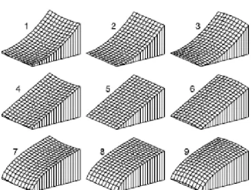
(13)Allowing n (which defines profile curvature) to assume values less than, equal to, or greater than 1 and ω (which defines plan curvature) to assume either positive, zero or negative values, one can define nine basic geometric reflief forms (Dikau R. [10]). Figure 7 illustrates nine basic hillslope types that are formed by combining three plan and three profile curvatures.
It is important to precise that, in this study, we focus on the shape of a hillslope in the length direction, while considering the distance (not shape) in the width direction. However, the distance in the width direction is a direct consequence of both profile and plan curvature, since these determine the location of the slope divides. The location of the slope divides as well as some contours are shown in figure 8. Thus the values of parameters n, ω and H are different for each of these nine hillslope types.
As a consequence, there is a major observation that is to be made concerning the width function: Because of the amalgam that is made between the hillslope’s width and its plan curvature, the variation of the width function is directly linked to the convergence or divergence of flow on the hillslope. In other words, an increasing width function from the top divide to the river implies a divergent flow on the hillslope, and a decreasing width function implies a convergent width function. Moreover, because of simplification of the HSB model from a 3-D to a 1-D model, one single flow direction can be considered on the hillslope. Let us now assume that that width function of a given hillslope is non-monotonic (figure 11). Thus, the flow is divergent when the width function increases and convergent when this function decreases. It is obvious the configuration of figure # cannot be real as far as hydrology is concerned. In particular, according to a hillslope’s definition, flow has to be convergent at least in a limited area along the edges of the hillslope.
For a width function to meet 1-D Boussinesq’s requirements, it thus has to be monotonic. It is then necessary to inquire about plan curvature which is going to tell us whether the flow is convergent (concave plan curvature) or divergent (convex plan curvature). The hillslope’s width function will have to be decreasing if the flow is convergent, and it will have to be increasing if the flow is divergent.
2.4 LANDMAPR
MacMillan (2003a) [12] developed the software LandMapR which purpose is the automatic extraction of spatial entities from a DEM. Cécile Doukouré (2005) [12] presented the software: It is made of four distinct programs. Each calculation step corresponds to a program (figure 10).
Let us precise that LandMapR must be coupled with a GIS since it does not have any visualization system. Here is the purpose of each program:
• FlowMapR extracts the hydrographical network and defines the watershed’s boundaries using the DEM.
• FormMapR calculates derivatives that enable to describe the ground morphology, the orientations, slopes and that are going to be used as a basis to classify the area.
• FactMapR establishes a concrete classification of ground curvature (flat, concave or convex – see IV.2.3.3). LandMapR uses a fuzzy logic to classify the area. In other words, a geographical entity will not be classified simply as concave or convex but some thresholds are defined so that some other fuzzy considerations can be made. For example, a geographical entity can be said relatively concave or highly convex.
• WeppMapR extracts hydrological entities required by the erosion model WEPP. In conclusion, this paper deals with the construction of two algorithms:
• On algorithm aims at dividing a watershed into hillslopes and at determining plan and profile curvature of every hillslopes
• Another algorithm aims at calculating the hillslope’s width function
The data acquired will enable to solve eq. (5) with an iterative method (finite difference method for example). The resolution itself is not tackled in this paper.
LandMapR, and more precisely the FormMapR module is a very interesting tool as far as our study is concerned. It enables to determine the curvature of a geographical entity. Moreover, the only data required is a DEM. Nevertheless, applying LandMapR on the rough DEM may return some non-logical results namely because the calculated river network does not correspond to the real one. We will see in IV.1 that PHYSITEL considers the real hydrological network which enables the INRS’s software to produce data that are closer to the hydrological reality.
The problem is that PHYSITEL is not able yet to calculate derivatives using the DEM in order to classify the area according to its morphology. This paper describes the construction of the extension algorithms that will enable PHYSITEL to do the same job as LandMapR adding hydrological considerations in its calculation method.
3
METHOD
3.1 PHYSITEL
The only data used during this study was provided by the GIS PHYSITEL 3.0. developed by A. Royer, A.N. Rousseau, S. Savary, J.-P. Fortin, R. Turcotte at the INRS-ETE (Institut National de Recherche Scientifique – Eau, Terre et Enviornnement) in Quebec. PHYSITEL enables to determine the flow structure in a watershed. To do so, it requires:
• a DEM (Digital Elevation Model)
• a hydrological network as a vector network • a land use map
• a soil type map
Our study did not require any data concerning land use or soil type.
There is no limit to the resolution and dimension of the DEM with PHYSITEL. The user can largely add different types of map projections. The vector network is used together with the DEM in order to determine more precisely the flow directions in flat lands and to identify lakes and reservoirs that cannot be detected by the DEM.
Once the flow structure is determined with a given resolution, PHYSITEL can divide the watershed into Relatively Homogeneous Hydrological Units (RHHU). Each RHHU is made of the set of pixels ‘flowing down’ to a river segment generated by PHSYSITEL. A river segment is limited by two confluences, or by one confluence and one head water point, or by one confluence and the watershed outlet (figure 13).
It is then possible to divide each RHHU of a given watershed into hillslopes as described in III.2.1. Moreover, PHYSITEL can provide several data matrices:
• The elevation matrix • The flow direction matrix • The RHHU matrix
• The Channel network matrix
We will describe these matrices in part IV.2.1.2. Only these matrices will be used as input parameters to produce the data required by the HSB model (profile curvature and width function).
3.2 CHOICE OF A PILOT WATERSHED
3.2.1 Presentation
The study concerns the BEREV (Bassin expérimental du Ruisseau des Eaux-Volées) watershed. This watershed covers 9.2 km2 (922 ha) and it is located at 47°16’20”N, 71°09’40”W, that is to say
approximately 80 km north of Quebec City. It is part of the Montmorency forest in the Laurentides Mountain Range. This watershed was chosen because of its rapidly varying topography.
Figure 14 is a map of the area that enables to pinpoint the BEREV basin.
3.2.2 Modelling
The watershed was modelled using PHYSITEL 3.0 and a digital elevation model (DEM) built with 5m×5m pixels.
Figure 15 presents the basin on a screen shot produced by PHYSITEL, which displays the elevation on the area.
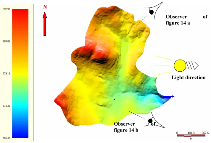
Figures 16 and 17 illustrate this watershed in 3-D. These pictures were obtained using Global Mapper 6:
In figure 16 and 17, please refer to figure 15 to acknowledge the respective positions of the observer. Also, let us precise that, concerning light direction, sun makes an angle of 45° with the horizontal level and it azimuth the 90° with the North direction. In other words, sun is shining from the East.
3.2.3 Dividing the watershed into RHHU
We chose to divide the basin into 13 RHHU, based on a network threshold of 10000 meshes (25 ha) so that a stream can be considered as a river segment, and a RHHU threshold of 20 pixels minimum (0.05 ha) so that a set of pixels can be regarded as a RHHU. The hydrological units remain quite large and their shapes are friendlier.
Figure 18 is a map displaying the division of the basin into 13 RHHU:
Table 1 gives the area of each RHHU calculated with Physitel (counting the number of pixels on each RHHU and multiplying this number by the resolution of one pixel).
Table 2 gives the total area of the BEREV watershed and the mean RHHU area.
Let us precise that the division of the basin into RHHU entirely depends on the hydrological behaviour of the watershed. As a matter of fact, the higher the river network resolution, the greater the amount of RHHU. Thus, there is only one channel in each RHHU. In other words, a RHHU is entirely defined by the channel that belongs to this hydrological unit.
3.3 Form calculation for every hillslopes of the BEREV watershed
3.3.1 Available data 3.3.1.1 Algorithms
The calculation of a RHHU’s hillslopes’ form is done by 2 or 4 different algorithms depending whether a head water or intermediate RHHU is studied. The algorithms were written using Matlab
6.5. They will be translated into C++ language so that they can be used by PHYSITEL as an extension. Here are the algorithms created:
• Forme_transversale_lateral: Calculates plan curvature of lateral hillslopes for every kinds of RHHU.
• Forme_longitudinale_lateral: Calculates profile curvature of lateral hillslopes for every kinds of RHHU.
• Forme_transversale_tete: Calculates plan curvature of head hillslopes for head water RHHUs.
• Forme_longitudinale_tete: Calculates profile curvature of head hillslopes for head RHHUs.
The algorithms will be available and the access free on the local network.
3.3.1.2 Data requirements
Each of the afore mentioned four algorithms is a function of 5 different matrices produced by PHYSITEL. They are all the same dimensions and can be stacked. In the example of the BEREV watershed each matrix is made of 825 lines and 799 columns:
• The elevation matrix: it displays the elevation of each pixel located within the basin. The value -∞ (-9999.99) is given to pixels beyond the watershed boundaries
• The flow direction matrix: On each pixel of the basin, the value indicates the downstream pixel. This value is an integer of the interval [1; 8]. The figure below displays the way such a value is given to one pixel:
The value 0 is given to the pixels beyond the watershed boundaries.
• The RHHU matrix: It contains the ID number of the RHHU (1 to 13) on the pixels that are in the basin. The value 0 is given to the pixels beyond the watershed boundaries.
• The Channel network matrix: Only the pixels located on the river segments are given the number of the RHHU the channel is associated with. The value 0 is given to every other pixel.
• The head water hillslope matrix: It looks like the RHHU matrix but the remaining non-zero pixels are located on the head water hillslopes of the head water RHHUs of the basin. The value 0 is given to all other pixels.
The first four matrices can be produced by the present version of PHYSITEL. Only the production of the head water hillslope matrix requires another small algorithm called ‘head_pixels’ that is a function of the first four matrices only and that is looking for the head pixel of a river section included in each head water RHHU.
In figure 20 are circled the head pixels of the channel network of the BEREV watershed. Thus, RHHU 3, 5, 6, 8, 11, 12 and 13 are head water RHHUs (see also fig. 18). In other words not only can this program single out head water pixels, it can also identify the head water RHHUs which is going to be major information in the general program.
Table 3 is the result of the ‘head_pixels’ algorithm for the example of the BEREV watershed:
The first line indicates the number of the head water RHHU, the second line indicates the line of a head water pixel in the RHHU matrix and the third line indicates its column.
It is then possible to look for all flow paths that end to one given head pixel, so that PHYSITEL can return the head water hillslope matrix. We can thus define a head water hillslope mathematically: It corresponds to the set of pixels that are crossed by flow paths that end to one given head water pixel.
3.3.2 Dividing each RHHU into hillslopes
A curvature calculation will be made for each RHHU. A loop will run from the RHHU #1 to the RHHU #13. Without loss of continuity, we present here the calculation for only one RHHU.
A program first has to divide each RHHU into two (intermediate RHHU) or three hillslopes (head water RHHU).
3.3.2.1 Hillslope characterization
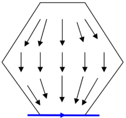
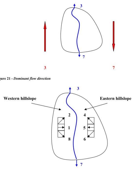
Given the channel network matrix, we first have to calculate the dominant flow direction of the river segment. To do so, we count the number of times each direction value (1, 2, 3, 4, 5, 6, 7, or 8) occurs. The dominant flow direction, called ‘dirdom’, is set to the most frequent flow direction. For example, let us consider the intermediate RHHU of figure 18:
In that case, the dominant flow direction may hold the value 3 or 7. What is important is that the flow direction is vertical because the fact that water flows towards North or South in the river does not interfere on the flow directions on the hillslopes.
Now, the aim is to use a hydrological criterion to make a distinction between two lateral hillslopes. At this point, no distinction is made between lateral and head water hillslopes. This distinction is going to be made in the next step of the calculation.
Figure 22 enables to understand the hydrological criterion we use:
We consider that, on one given lateral hillslope, the three possible flow directions that directly point towards the river section identify the pixels that belong to the hillslope located in the opposite side of the channel. If we consider the example of figure 19, with a river flowing in the direction 3 or 7, the flow direction matrix’ pixels holding the values 4, 5 and 6 single out the eastern hillslope while the pixels with the values 2, 1 or 8 pinpoint the western hillslope.
Nevertheless, the pixels with the values 3 or 7 may belong to either the western or the eastern hillslope. That is the reason why we first decided not to consider those pixels to characterize a hillslope. As a consequence, the hillslope matrix will contain some holes. Figure 23 displays an example of a breached hillslope. The hillslope’s shape was chosen arbitrary.
Then we just label those pixels like the rest of the hillslope in the half-space defined by the line passing through the two extreme points of the RHHU and the given hillslope (figure 24).
Besides, a few pixels may be assigned a flow direction value whereas they do not belong to the original hillslope. This gives birth to clusters of parasitic pixels (figure 25)
In order to cope with such clusters of parasitic pixels, we decided to put the value 0 on the pixels located in the other half-space (figure 26).
But a few pixels (highlighted in yellow in figure 26) that actually belong to the original hilllsope may be overlooked because they are located in the other half-space. We assume that the corresponding number of pixels is negligible considering the total number of pixels on the hillslope.
Let us finally precise that some pixels in the original hillslope may be assigned a flow direction that is non compatible with the hillslope. Nevertheless, those pixels belong to the studied hillslope, so we add them to the hillslope matrix (figure 27).
For the example of the southern hillslope of intermediate RHHU #1, here are two figures that show the breached hillslope (28a) and the clean hillslope (28b).
To put in a nut shell, once a given hillslope is identified with the criterion described in figure 15, here are the three kinds of special pixels we have to deal with in order to create a clean hillslope matrix:
• Holes due to parallel flow directions of pixels located in the half space that corresponds to original hillslope
• Holes due to non-compatible flow directions of pixels located in the half space that corresponds to original hillslope
• Clusters of parasitic pixels due to wrongly compatible flow directions of pixels located in the other half space
Figure 29 describes the boundaries of the original hillslope
3.3.2.2 Hillslope elevation matrix
Once a RHHU is divided into two ‘hillslopes’ labeled differently, a distinction has to be made between head water and lateral hillslopes. Thus we use the head water hillslope matrix and the information provided in table 3 (called T in the algorithm) to single out the head RHHU, the head pixel in each head RHHU and the pixels that belong to the head hillslope. The calculation method varies from one algorithm to another and whether we study an intermediate or a head water RHHU:
• If the RHHU is intermediate, there is no head water hillslope so the program will not spot any pixel and the RHHU is already divided into two lateral hillslopes.
• If the RHHU is a head water RHHU, and if we consider the lateral hillslope calculation algorithm, then the algorithm will erase the values (put 0 instead) in the pixels that belong to the head water hillslope. As a consequence, the remaining matrix can be treated just like a regular intermediate RHHU matrix.
In the 2 latter cases, the algorithm will then code the two hillslopes with two different values: 1 and 2. As a consequence, we have a new matrix that contains 1 on the pixels that belong to the hillslope #1, 2 on the pixels that belong to the hillslope #2 and 0 elsewhere. We can also obtain one matrix per hillslope, replacing 1 or 2 by 0.
• If the RHHU is a head RHHU, and if we consider the head hillslope calculation algorithm, then the algorithm will just use the head hillslope matrix to isolate the required hillslope. Thus we have a matrix where only the considered head hillslope is coded with the RHHU number.
Finally, the code on each hillslope is replaced by the elevation of each pixel, stacking the given hillslope matrix on top of the elevation matrix. Every other pixels that are not part of the given hillslope got the value 0.
It is possible to plot this kind of matrix with Global Mapper 6 to get an idea of what the hillslope looks like. Some visual results will be displayed in V.1.6.
3.3.3 Calculating plan and profile curvatures for each hillslope
3.3.3.1 Presentation
Once we have a hillslope elevation matrix, we look for elevation lines that are parallel or perpendicular to the flow direction depending whether we want to calculate the plan or profile curvature of this hillslope respectively. The goal is to obtain an elevation lines matrix. Each line of this matrix will be studied as an elevation function. Studying its second derivative’s sign, it is possible to deduce the curvature of each elevation line. As a consequence, we can have some clues about the entire hillslope plan and profile curvatures.
3.3.3.2 Creating an elevation lines matrix for each hillslope
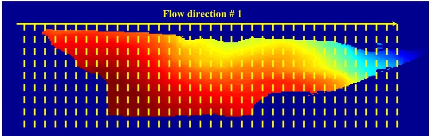
Figures 30 & 31 illustrate the method of the elevation lines catchment for the example of RHHU #1, south hillslope:
The algorithm will scan the matrix and gather the elevation lines parallel to the dominant flow direction, that is to say horizontal in this example. It is Important to precise that the program will overlook every elevation lines that contain less than 10 elevations values so that small clusters of pixels do not have any influence on the final result. This threshold has been chosen arbitrary. It means that a line which length is below 50 meters is not significant as far as the curvature calculation is concerned. We will discuss about different methods to determine this threshold according to a hillslope’s size parameters or according to the curvature calculation theory in part V.1.8.
The algorithm will scan the matrix and gather the elevation lines perpendicular to the dominant flow direction, that is to say vertical in this example.
Plan and profile curvature calculations are concerned by two different algorithms. In each case, we obtain an elevation lines matrix which lines are made of the elevation lines gathered.
3.3.3.3 Calculating plan and profile curvatures for each elevation line
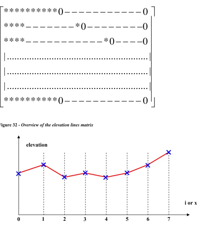
A * represents an elevation value. The dimension of the matrix depends on its construction: As a matter of fact, the number of lines in the matrix depends on how many non zero lines the algorithm is able to find in the hillslope matrix, and the number of columns depends on how many non-zero elevation values the algorithm is able to find in a row.
Each line in this matrix is studied as a given discrete function. Figure 33 illustrates this kind of elevation line function:
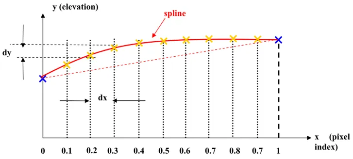
We will first interpolate this discrete function using the ‘interp1’ function of Matlab. If x is the column index matrix corresponding to an elevation line, and y is an elevation line vector, then ‘yi = interp1(x,y,xi)’ returns the vector yi containing elements corresponding to the elements of xi and determined by interpolation within vectors x and y. The vector x specifies the points at which the data y is given. We decided to divide each unit interval of x into 10 intervals, each of them being 10 times as small as one interval of x.
yi = interp1(x,Y,xi,method) interpolates using alternative methods. We chose the cubic spline interpolation displaying ‘spline’ as the interpolation ‘method’. You will find a detailed article concerning the theory of the cubic spline interpolation as reference [13].
Let’s zoom on one unit interval of x. Figure 34 illustrates the cubic spline interpolation method:
We now consider the obtained discrete function. Given the slpine’s properties, we know this function can be derived twice. Thus we consider the second derivative on each interval of the splined elevation function:
Be xi the abscise point # i and yi the corresponding elevation point. Thus for i∈[1, length of elevation line - 1], the first derivative can be written:
1 1 i i i i
y
y
dy
dydx
dx
x
x
+ +−
=
≡
−
(14)‘dydx’ is the first derivative vector. It gives the slope of the interpolated function on each interval [xi, xi+1] (figure 35).
Besides, we obtain the vector dy made of the elevation variation for each step.
We can now calculate the second derivative of the elevation function:
1 2 2 1
2
2
2
(
)
i i i idy
dy
d y
d ydx
dx
x
x
+ +−
=
≡
−
(15)Let us precise that it can run from 1 to the length of dx – 1 that is to say the length of x or dy – 2 since we are loosing a calculation point each time we derive a function.
We obtain the second derivative vector ‘d2ydx2’ and the next step consists in studying the sign of the values this vector is made of:
• A negative value corresponds to a decrease in the first derivative function, that is a decrease in the slope value. Thus a negative value of the second derivative vector should correspond to a concave curve. Nevertheless, we are interested in the ground curvature. That is why a concave elevation function implies a convex ground line. Figure 36 illustrates this new definition we give to a concave ground line:
• Likewise, a positive value corresponds to an increase in the first derivative function, that is an increase in the slope value. Thus, a positive value of the second derivative vector should correspond to a convex curve. Nevertheless, we are interested in the ground curvature. That is why a convex elevation function implies a concave ground line. Figure 37 illustrates this new definition we give to a convex ground line:
You will find the complete theory of convexity in reference [14].
Thus we count how many times positive and negative values appear in the vector d2ydx2. We use the basic following criterion:
‘If the number of positive values in the vector d2ydx2 is strictly superior to the number of negative values, then the ground line is said to be concave. If there are as many positive values as negative values, then the line is said to be
straight. Otherwise, it is said to be convex’.
3.3.3.4 Deducing the plan and profile curvature for each hillslope
We now consider the entire hillslope where every elevation line’s curvature has just been determined. Likewise, we count the number of convex and concave elevation lines:
‘If the number of convex elevation lines is strictly superior to the number of concave lines, then the hillslope is said to be convex. If there are as many convex lines as concave lines, then the hillslope is said to be straight. Otherwise, it is said to be concave’.
3.4 Width function calculation for every hillslopes of the BEREV
watershed
3.4.1 Hillslopes interpolation
The principle of the calculation is quite simple. Let us first remind that the width function w(x) is a function of the length running from the top divide of the hillslope to its river segment. We saw in part III.2.3 that a width function has to be monotonic. Moreover, an increasing or decreasing width function is directly linked to a divergent or convergent flow on the hillslope, respectively.
Given those considerations, the first – but not the least – calculation step is the interpolation of the real shape of the hillslope. Segments are used to interpolate the hisllslopes. Two different methods of interpolation were developed whether a head or a lateral hillslope is concerned.
Let us precise that one will always be able to stack the real hillslope’s matrix and the interpolated hillslope’s matrix. As a consequence, the coordinates of the same pixel in these two matrices are the same.
• A concave hillslope in the plan direction implies a convergent flow on the hillslope. Thus, according to the considerations of part III.2.3, the width function has to be decreasing from the top divide to the river segment.
• A convex hillslope in the plan direction implies a divergent flow on the hillslope. Thus, according to the considerations of part III.2.3, the width function has to be increasing from the top divide to the river segment.
3.4.1.1 Interpolating a lateral hillslope
Before interpolating the hillslope, the flow nature (e.g. convergent or divergent flow) on the hillslope has to be defined in order to know whether the width function has to be increasing (e.g. divergent flow) or decreasing (e.g. convergent flow). The form calculation results are used in order to determine the plan curvature of the given hillslope:
As a consequence, we chose to interpolate each lateral hillslope with a trapezoid. Let us take the example of a North lateral hillslope (figure 38).
If the form calculation program returns a concave plan curvature, then the width function has to be decreasing from the top divide to the river segment.
The first step is to pinpoint the two extreme points of the river segment using a small algorithm
included in the width function calculation algorithm (figure #).
Since the flow direction on the river is horizontal, we decide that the two parallel sides of the trapezoid have to be horizontal as well. One of those two parallel sides interpolates the river segment. Nevertheless, there is little chance that A and D are on the same horizontal line. As a
consequence, figure 40 explains the definition of points AA and DD that are crossed by this interpolation segment.
Second step: Once the river is interpolated, the non parallel sides of the trapezoid are used to define the
divergence (e.g. increasing) or convergence (e.g. decreasing) of the width function. In the case of a concave plan curvature, we know the width function has to be decreasing.
The real hillslope shape is considered and the extreme column indices are looked for. In other words, the algorithm will scan the real hillslope’s matrix and pinpoint the coordinates of the non zero pixels which hold the minimum (cmin) and the maximum (cmax) columns indices respectively (figure 41).
Then, given the fact that the width function has to be decreasing from the top divide to the river segment, the algorithm will test the respective position of B, AA and C, DD.
Let us define cB, cAA, cDD and cC as the column indices of B, AA, DD and C respectively:
if cAA<cB and cDD>cC, then second and third interpolation segments of the hillslope pass through AA, B and DD, C respectively (figure 43).
if cAA>cB or cDD<cC (see example on figure 43), then the algorithm is going to single out the coordinates of the non zero pixels with the minimum line index (lmin). The corresponding column index (clmin) is determined as well. Figure 44 shows how the obtained point is used to define DDbis and C bis (if clmin < (cDD+cAA)/2, example of figure 41) or AAbis and Bbis (if clmin > (cDD+cAA)/2, example non developed in this paper).
In figure 44 we can see that a new column index is defined. It is calculated as the mid column index between cDD and clmin. It is thus possible to define DDbis and Cbis:
Î cDDbis = (cDD+clmin)/2 and lDDbis = lDD Î cCbis = cC and lCbis = lmin
Finally, we can define the line passing through Cbis and DDbis. Translating it so that it passes through DD and drawing the line with the opposite slope and that passes through AA, it is thus possible to define the second and third segments as described in figure 45.
Third step: In order to isolate the interpolated hillslope’s matrix, a new matrix (called D in the
algorithm) is created. Its pixels hold the value 1, 2 or 3 inside the interpolated surface of a #1, #2 or head hillslope, respectively. The value 0 is held by the pixels located beyond the interpolated hillslope’s boundaries. Thus, at this step, given a starting D matrix full of non zero pixels (holding the value 1, 2 or 3), the algorithm will put zeros under line (DD AA), on the left side of line (DD C) or (DDbis Cbis) passing through DD, and on the right side of line (AA B) or (AAbis Bbis) passing through AA (see step 1 to 3 in figure 47.
The fourth interpolation segment is supposed to interpolate the top divide and is to be parallel to the river interpolation segment. The algorithm will use the area criterion to define this segment: As a matter of fact, the algorithm will first count the number of non zero pixels inside the three first boundaries of the interpolated hillslope (using the D matrix – see step three in figure 44). Then it will do the same with the real hillslope (using the real hillslope’s matrix) and compare the two areas. At step 3 of figure 47, the corresponding area of the interpolated surface has to be bigger than the real hillslope’s area. So as long as the interpolated area is bigger than the real one, the algorithm will put zeros upon the horizontal line which index increases form 1 to the accurate line index with the calculation step 1.
Figure 46 sums up the principle of the afore explained loop and figure 44 sums up the entire principle of interpolation.
If the form calculation program returns a convex plan curvature, then the width function has to be increasing from the top divide to the river segment.
First step: It is the same as the first step for a decreasing width function. In other words, the
algorithm first pinpoint the extreme points on the river segment the same way as it does for a decreasing width function (see figures 39).
Second step: This time, the algorithm will first single out the point that belongs to the real
hillslope’s and with the minimum line index lmin (figure 48). Let us call Cbis the corresponding extreme point.
If clmin > cDD and clmin < cAA, that is to say if Cbis is located between DD and AA, then it is possible to define the slopes of the second and third interpolation segments:
Î if clmin < (cDD+cAA)/2, then the third interpolation segment is defined by the line which slope is half the slope of the other line that passes through DD and Cbis (figure 49).
Î if clmin < (cDD+cAA)/2, then the second interpolation segment is defined by the line which slope is half the slope of the other line that passes through AA and Cbis (example non developed in this paper).
Let us precise that we had to divide the slope of the non parallel sides of the trapezoid by two, otherwise the area of the interpolated surface would decrease rapidly and give a smaller surface than the real one as soon as zeros are put beyond the interpolated surface’s boundaries, without any area comparison.
The second or third interpolation segment, respectively, is thus defined by the line of opposite slope passing through AA and DD respectively (figure 49).
If clmin < cDD or clmin > cAA, that is to say if Cbis is not located between DD and AA, then The following construction is to be made:
We define a new slope p3 which is the mean slope between p1 (line passing through DD and Cbis) and p2 (line passing through AA and Cbis):
1 2
3 2
p p p = +
We will then use this new slope p3 to draw the second interpolation segment that passes through AA with the slope p3.
The third interpolation segment passes through Cbis and DD. We obtain the interpolation described on figure 51.
Third step: The algorithm will now compare the area of the interpolated hillslope of figure 48 to the
area of the real hillslope:
• If, at the initial calculation step, the interpolated area is bigger than the real area, then as long as the afore mentioned statement is true, p3 will be decreased as follow (figure 52.):
1 2
3 0.1
2 p p
p with q q at each calculation step q
+
= = +
+
• If, at the initial calculation step, the interpolated area is smaller than the real area, then as long as the afore mentioned statement is true, p3 will be increased as follow (figure 53):
1 2
3 0.1
2 p p
p with q q at each calculation step q
+
= = +
−
3.4.1.2 Interpolating a head water hillslope
In that case, there is no use determining the flow nature since we know it has to be convergent. Part III.2.1 namely reminds that every flow paths on a head water hillslope end at a single point which is the head water pixel of the outlet river. As a consequence, dealing with a head water hillslope implies that the width function has to be decreasing.
First step: We use the ‘head_pixels’ algorithm (see IV.3.1.2) to pinpoint the head water pixel on each
head water hillslope. We obtain the point A.
Second step: Two other points B and C have to be defined on the real hillslope in order to define the
two first interpolation segments. To do so, the algorithm will look after extreme points defined by extreme line or column indices. The extreme indices that are considered depend on the dominant flow direction in the outlet river. Table 4 gives the extreme points that are considered for every flow directions.
Let us remind that lmax, lmin, cmax, cmin, correspond to the maximum line index of a non zero pixel, the minimum line index of a non zero pixel, the maximum column index of a non zero pixel, and the minimum column index of a non zero pixel, respectively. clmax, clmin, lcmax and lmin are de corresponding column and line indices.
Let us take the example of a head water hillslope with a dominant flow direction in the outlet river holding # 1 (figure 54).
Then zeros are put above (A C) and below (A B) in a D matrix that had been filled with threes. (see concave lateral hillslope – third step).
Third step: The aim is to find the third interpolation segment. For the purpose of the width function
calculation, this segment has to be perpendicular to the dominant flow direction in the outlet river. Calculating the width function, the algorithm will namely scan the final D matrix in this perpendicular direction from the interpolated top divide to the outlet river since this perpendicular direction is said to be the dominant flow direction on the hillslope as well.
Thus, the area criterion is used to build this interpolated top divide. The method is the same as described for a lateral hillslope’s interpolation (see concave lateral hillslope – third step). In other words, the third interpolation segment is given by the D matrix boundaries for the time being. Then a first area comparison is made and a loop will insert zeros in the D matrix in the direction of the interpolated top divide (perpendicular to the dominant flow direction) beyond this segment. Zeros are inserted in the D matrix as long as the interpolated hillslope’s area is bigger than the real hillslope’s area. We obtain the final D matrix (figure 55) which is going to be used in order to calculate the hillslope’s width function.
3.4.2 Building the width function values column 3.4.2.1 Looking for width measurement lines
Let us remind that, once the real surface is interpolated, a new matrix, called D, is created. It is made of non-zero values on the interpolated surface – basically the code of the hillslope (# 1, 2 or 3) – of a given hillslope, and zeros beyond the interpolated hillslope’s boundaries. The algorithm is now able to measure the width function values, counting non zero values on each line of the D matrix, parallel to the dominant flow direction for lateral hillslopes, and perpendicular to the flow direction for head
hillslopes. Figure 56 gives an illustration of the D matrix for a lateral hillslope which river has a dominant flow direction # 1.
Let us precise that no hole and no parasitic pixel can be found neither in the hillslope matrix nor in the D matrix since the hillslope characterization correction was made (see IV.2.2.1).
3.4.2.2 Determining the width values column
Each width function value is then stored in a vector that is a column containing all the width function values (figure 57).
Let us precise that every time the algorithm is looking for non-zero values it may cover the matrix in one given way and the width function column may display values in the reverse order. If we take the example of a south lateral hillslope with a horizontal dominant flow direction in the river, the program will scan the D matrix the same way as it does with a north hillslope. As a consequence, we just reverse the values in the obtained column so that a width function column always displays width values from the top divide to the outlet river (head water hillslope) or the river segment (lateral hillslope).
Finally, concerning the case of the width function calculation on a head hillslope, the program will look for non-zero values along lines that are not parallel but perpendicular to the dominant flow direction in the outlet river (figure 58).
3.4.2.3 Definition of the step in a width function column and effective width values calculation in meters
Finally, we have to precise what is the step between two width values in a width column. This step depends on the dominant flow direction for a given river segment:
• If the dominant flow direction is ‘straight’ that is to say horizontal or vertical (direction # 1, 3, 5 or 7), then the gap between two width lines is the side of one pixel. As a consequence, the step between two width values in the width column equals the resolution of the BEREV mapping with PHYSITEL, that is to say 5 m. Moreover, every time we have a number of non-zero values on one line of the D matrix, we have to multiply it by 5 to obtain the corresponding width in meters (figure 59).
• If the dominant flow direction is ‘diagonal’ (direction # 2, 4, 6 or 8), then the gap between two width lines is a bit smaller than before: it is half the size of a pixel’s diagonal, that is to say 0.5* 2. So the step between two width values in the width column is 0.5* 2*5 with PHYSITEL mapping, while the coefficient we have to multiply by a number of non-zero pixels on one width line is larger: It is the size of a pixel’s diagonal, that is to say 5 2 meters (figure 60).
4
RESULTS AND DISCUSSION
4.1 Form calculation
In the following tables, CV = convex, CC = Concave.
N, S, E and W stand for North, South, East and West respectively as far as the plane orientation of each hillslope is concerned (e.g. on a plane map). These ought not to be mistaken with a flow direction holding an integer value of the interval [1:8].
4.1.1 Plan curvature for lateral hillslopes
# UHRH 1 2 3 4 5 6 7 8 9 10 11 12
dominant flow direction 1 7 8 7 7 5 1 8 2 1 8 2
hillslope # 1 form CV CV CV CC CC CV CC CV CC CC CC CV % convex hillslope 1 63 75 61 41 34 77 34 50.4 46 48 44 86 % concave hillslope 1 37 25 39 59 66 23 66 49.6 54 52 56 14 orientation of hillslope 1 S E NE E E S S NE SE S NE SE hillslope # 2 form CC CC CC CC CV CC CC CC CC CC CC % convex hillslope 2 5 6 4 4 65 32 9 12 14 2 6 % concave hillslope 2 95 94 96 96 35 68 91 88 86 98 94 orientation of hillslope 2 N W SW W W N N SW NW N SW NW
4.1.2 Profile curvature for lateral hillslopes
# UHRH 1 2 3 4 5 6 7 8 9 10 11 12
dominant flow direction 1 7 8 7 7 5 1 8 2 1 8 2
hillslope # 1 form CV CV CV CV CV CC CV CV CV CV CV CV % convex hillslope 1 83 74 84 83 77 30 72 69 84 64 76 89 % concave hillslope 1 17 26 16 17 23 70 28 31 16 36 24 11 orientation of hillslope 1 S E NE E E S S NE SE S NE SE hillslope # 2 form CC CC CC CC CC CC CC CC CC CC CC % convex hillslope 2 21 4 3 27 47 12 28 10 12.5 5 16 % concave hillslope 2 79 96 97 73 53 88 72 90 87.5 95 84 orientation of hillslope 2 N W SW W W N N SW NW N SW NW
4.1.3 Plan curvature for head hillslopes
# UHRH 1 2 3 4 5 6 7 8 9 10 11 12 13
head hillslope form CC CC CV CV CC CC CV
% convex 36 43 70 61 38 12 52
% concave 64 57 30 39 62 88 48
orientation NW N E NW NW SW S
4.1.4 Profile curvature for head hillslopes
# UHRH 1 2 3 4 5 6 7 8 9 10 11 12 13
head hillslope form CV CV CC CC CC CV CV
% convex 51 58 44 49 44 60 76
% concave 49 42 56 51 56 40 24
orientation NW N E NW NW SW S
4.1.5 Discussion about head water hillslopes plan curvature
Since a head hillslope is hydrologicaly defined by the head water pixel of a river segment where every flow paths of the given head water hillslope end, it is not possible to have a purely convex head hillslope as far as the plan curvature is concerned. Otherwise, the flow would be divergent and there would not be a single pixel as an outlet.
Nevertheless, we can observe in the latter tables that the plan curvature of some head hillslopes is said to be convex (head hillslopes in RHHU # 6, 8 and 13 – see red circles in table 7). As a matter of fact, even though a head hillslope has to be concave in the plan direction, some ground structures cannot be overlooked. Those structures may be convex and thus play an important role in the plan curvature calculation. Figure 61 is a 3-D plot of the head hillslope of the RHHU # 6.
On this mesh, it is possible to highlight a major convex ground structure. This structure weighs heavily in the plan curvature calculation as well as in the profile curvature calculation. Adding a medley between medium and small convex and concave structure on the hillslope, the algorithm returns a convex plan form with 70 %.
As a consequence, a head hillslope curvature calculation result is not to be taken as the real form of the hillslope but as the most important contribution of a given type of ground structure (convex or concave) to the general form of the hillslope.
4.1.6 Visual results
Hereafter are shown some figures (61 to 64) of some hillslopes using Global Mapper 6. Those pictures enable us to validate the statistical results returned by the algorithm:
Example: RHHU # 9 – North-West hillslope : According to the results of the algorithm, this
hillslope is said to be concave in the plan direction as well as in the profile direction:
Figure 62 displays the hillslope. It is possible to acknowledge the plan concavity of this hillslope given the shape lines we drawn. The latter lines are supposed to be parallel to the outlet river. As a consequence, looking at the hillslope in 3-D enables us to see that it is concave in a great deal, even though one can observe some small convex areas. Thus, the convex weight is only 12 % whereas the concave weight is 88 % for the plan curvature of this NW hillslope of the RHHU # 9.
Figure 63 displays the same hillslope but we are now interested in the profile curvature. Some shape lines have been drawn. They are supposed to be perpendicular to the river outlet and thus parallel to the flow direction. On can remark that one small convex area separates the hillslope into two major concave area. Nevertheless, the hillslope remains concave in the profile direction with a similar gap between the concave and convex weights (respectively 90 % and 10 %).
Below are some illustrations of the same hillslopes with some shape lines in grey shading. It may be easier to understand:
4.1.7 Fuzzy or binary logic?
We can see that tables 5 to 8 classify a hillslope as being concave, convex of flat. A priori, the algorithm uses a binary logic to determine the form of a hillslope. Moreover, we know that a binary result is required for the purpose of HSB model as Trcoh et Al. 2002 [5] explained that the n parameter will depend on the plan curvature and will take different values wether the corresponding hillslope is concave, convex or straight. But a relatively concave hillslope will be given the same n value as a highly concave hillslope, for example.
Nevertheless, the percentage of concavity and convexity is calculated in each case. It is thus possible to use a fuzzy logic for some other purposes, simply programming the required thresholds.
4.1.8 Choosing an elevation line threshold
The threshold is now set to 10 pixels. In other words, no elevation line smaller than 50 meters will be studied to calculate the curvature. Let us remind that the purpose of this threshold is to avoid calculating the curvature of small and thus non-significant clusters of pixels.
This threshold, that has been set arbitrary until now, can be calculated for each hillslope for example. The mean elevation line length can be calculated and the threshold could be a function of this mean.
On can also consider that the minimum elevation line length does not depend on the hillslope’s size, but depends on the curvature calculation theory. In other words, a minimum number of pixels may be required to define a discrete elevation function to derive.