HAL Id: hal-00304750
https://hal.archives-ouvertes.fr/hal-00304750
Submitted on 1 Jan 2002HAL is a multi-disciplinary open access archive for the deposit and dissemination of sci-entific research documents, whether they are pub-lished or not. The documents may come from teaching and research institutions in France or abroad, or from public or private research centers.
L’archive ouverte pluridisciplinaire HAL, est destinée au dépôt et à la diffusion de documents scientifiques de niveau recherche, publiés ou non, émanant des établissements d’enseignement et de recherche français ou étrangers, des laboratoires publics ou privés.
Simple sensors to achieve fine spatial resolution in
continuous measurements of soil moisture and salinity
F. Konukcu, J. W. Gowing, D. A. Rose
To cite this version:
F. Konukcu, J. W. Gowing, D. A. Rose. Simple sensors to achieve fine spatial resolution in continu-ous measurements of soil moisture and salinity. Hydrology and Earth System Sciences Discussions, European Geosciences Union, 2002, 6 (6), pp.1043-1051. �hal-00304750�
Simple sensors to achieve fine spatial resolution in continuous
measurements of soil moisture and salinity
F. Konukcu
1, J.W. Gowing
2and D.A. Rose
21Trakya Universitesi, Tekirdag Ziraat Fakultesi, 59030 Tekirdag, Turkey
2School of Agriculture, Food and Rural Development, University of Newcastle, Newcastle upon Tyne, NE1 7RU, UK
Email for corresponding author: [email protected]
Abstract
It is increasingly necessary to be able to measure, simultaneously, continuously and at fine spatial resolution, the salinity and water content of soil. This paper reports the design, construction, calibration and laboratory testing of two simple but robust instruments that enable this to be achieved. Salinity in solution was measured reliably, at 10-mm spacing, by multi-electrode resistivity probes up to saturation with NaCl (c. 6 mol l–1), though these probes required individual calibration and were unable to detect precipitated salt. Volumetric water content was
measured with great sensitivity over a wide range, from air-dryness (0.06 m3m–3) to saturation (0.55 m3m–3) in a sandy loam, using
thermal-conductivity probes that used a common calibration and were unaffected by the salinity of the soil solution, by temperature and by ageing.
Keywords: soil moisture, soil salinity, thermal-conductivity moisture probe, four-electrode salinity probe
Introduction
Irrigated agriculture in arid and semi-arid regions is widely perceived to be environmentally damaging. Better management is required to conserve water and decrease saline drainage discharge. This regime of leaching, together with increasing dependence on water of marginal quality, demands proper management of soil salinity. Thus, reliable and affordable methods of monitoring both soil salinity and soil moisture are required.
Sampling and laboratory analysis is not an attractive option because of the time and effort involved. Furthermore, in experimental column studies, the destructive nature of this technique is inappropriate. Conventional methods of in
situ soil-moisture monitoring using tensiometers and
resistance blocks are applicable over a limited range, while the latter are also affected by the variable salinity. Modern sensors are available commercially to determine bulk soil properties in the field (Rhoades, 1990, 1992) but these are relatively expensive and generally do not permit fine spatial resolution.
This paper describes the design, development and testing of two instruments for continuous, non-destructive
measurement of soil moisture and salt content, which are believed to have wide applicability in salinity research.
Soil-water content was measured using thermal-conductivity probes and salinity by multi-electrode resistivity probes. Both were designed, manufactured and adapted for the purpose of achieving fine spatial resolution during continuous measurement. Their construction and calibration are described, together with experiments to test their performance. The accuracy, reliability, stability and variability were tested over a wide range of moisture contents, at high salinities, and at different temperatures.
The instruments
MULTI-ELECTRODE RESISTIVITY (FOUR-ELECTRODE) PROBE
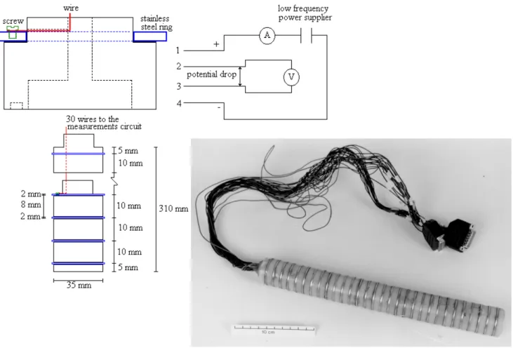
Each probe consists of a nylon tube, 35 mm in diameter and 310 mm long, having 30 stainless steel rings (each 2 mm thick) spaced equally (10 mm from centre to centre) along the probe. The rings are used as electrodes, and are connected to the measurement circuit via 30 electrical leads
F. Konukcu, J.W. Gowing and D.A. Rose
gathered in two plugs. Because each probe has 30 electrodes, the resistance can be measured at 27 points. However, only 24 positions could be interrogated because the leads from each electrode were gathered into two plugs and each plug had 12 switch positions (1,2,3,4; 2,3,4,5;...12,13,14,15; and 16,17,18,19... ; 27,28,29,30). The probe was filled with fibreglass to insulate the electrical leads (Fig. 1). A current can be applied across the outer pair of any four adjacent electrodes and the corresponding voltage drop is measured by a voltmeter between the inner pair.
THERMAL CONDUCTIVITY PROBE
Several designs have been described in publications referred to by Wechsler et al. (1965). More recently, Bristow et al. (1994 a,b) have developed probes for measuring the thermal properties of soil. Our design, based on the probe described by Fritton et al. (1974), is relatively easy to build, cheap and uses readily available materials, as well as being simpler and smaller than those of Bristow and his co-workers. Commercial probes are also available but are too large for fine resolution of detail. The thermal conductivity probes
described by Fritton et al. (1974) consist of a heater element, a thermocouple and a protective covering.
For the heater element, each end of a 310-mm length of 0.1-mm (42 standard wire gauge) minalpha wire, resistance 16 W m–1, was first fused to a 3-m length of 0.85-mm outside diameter (OD) wire lead. Each joint was then covered by a 10-mm length of 1.6-mm heat-shrinkable tubing. This heater wire was then folded in half and pulled through a stainless steel tube, 150 mm long, 0.8 mm OD and 0.5 mm inside diameter (ID). A small (0.1 mm) wire, which was used to pull the heater wire through the tube, was cut from the end of the tube and removed when the heater wire was in place. A K-type commercial thermocouple was used (RS components).
To stabilize the joints, a heat-shrink sleeving was shrunk over the heater and the thermocouple to keep them in close contact. The rigidity of the welded joints was increased further by fitting successively a 10-mm length of 4.8-mm diameter heat-shrink tubing on the lead-wire end of the probe and on the lead wires until a glass tube (60 mm long, 6.4 mm OD) fitted snugly over the lead wire completely. Epoxy cement was then inserted into the two ends of the glass
tubing and placed on the tip of the probe to seal the electrical connections from water. Further construction details are available from the corresponding author.
A multi-range microammeter was used to measure the current supplied and the temperature of the thermocouple was read by a digital thermometer to an accuracy of 0.1 K.
Theory
MULTI-ELECTRODE RESISTIVITY (FOUR-ELECTRODE) PROBES
By employing an appropriate cell constant, c, it is possible to determine the specific electrical conductivity from the resistance measurements and temperature (American Public Health Association, 1985) as:
[
1 0.00191( 25)]
1000 25=R + T− c E (1) whereE25 = electrical conductivity of the sample (dS m–1) at a reference temperature of 25°C;
R = measured resistance of the sample (W), R= V/I; V = potential difference between two inner electrodes (V); I = current (A) ;
T = temperature of the measurements (°C); and
c = cell constant (m–1), which represents the fraction of the specific resistance measured by the electrodes. If the probes are placed in a solution, the electrical conductivity of the solution is measured. However, if they are inserted into a moist soil, the electrical conductivity of the bulk soil, Ea , is measured. A further correction must be applied to the measured soil bulk electrical conductivity (Ea) because the desired electrical conductivity is that of the soil solution (Ew). The soil bulk electrical conductivity, Ea, depends upon the soil-water content, θ, the electrical conductivity of the soil ‘water’, Ew, and the electrical conductivity of the soil minerals, Es. The inter-relationships among these variables have been investigated on several occasions. Rhoades et al. (1976) assumed two parallel conducting elements or pathways, the liquid phase and the solid phase, in a linear model. This linear model, however, fails to describe adequately the relationship between Ea and
Ew (Nadler and Frenkel, 1980; Shainberg et al. 1980). In a three-component model, Rhoades et al. (1989) assumed a continuous solid, a continuous liquid, and a solid-liquid series-coupled element. The electrical conductivity of bulk soil, Ea, is expressed by this model as:
(
)
wc wc s ws s s ws w s E E E E E E θ θ θ θ θ + + + ws 2 s a= (2) whereEs = electrical conductivity of the soil particles (dS m-1). Rhoades et al. (1989) gave an empirical relation for Es based on the percentage clay content of the soil,
ϕ
, as:0.021 0.023
s ≅ ϕ−
E ;
Ews = electrical conductivity of solution in the ‘series-coupled’ pathway, (the finer pores containing ‘immobile’ water) (dS m–1);
Ewc =electrical conductivity of solution in the larger pores, (mobile water) (dS m-1);
θs = volumetric content of the soil particles which can be calculated from the relationship between soil bulk density, ρb , and soil particle density, ρs, as
s b s ρ ρ θ = ; θwc = volumetric content of the soil solution in the larger
pores, or so-called mobile water; and
θws = volumetric content of the soil water in the ‘series-coupled’ pathway (or immobile water).
Rhoades et al. (1989) partitioned the total soil water content, θ, into two fractions, mobile (θwc) and immobile (θws) water, where θ = θwc+ θws. They obtained θws from laboratory measurements on soil columns as
011 0 64 0
ws ≅ . θ + .
θ . The mobile fraction allows convective flow of water and solute in soil, whereas the immobile fraction remains essentially stagnant surrounding the soil particles and in small pores. But, because of the lack of any suitable method for determining the conductivity of the immobile solution, they assumed the same value of electrical conductivity, Ew, for these two different fractions. For transient movement of water through the soil, this assumption is obviously questionable, because the solute concentrations in these two types of soil solution are not the same under non-equilibrium conditions. But, when the flux is small in non-structured packed soil, these two values can be assumed equal. Rearranging Eqn. (2) with this assumption:
(
)
(
)
w ws w s w s s w s a E E E E E E θ θ θ θ θ θ + − + + ws 2 ws = . (3)Ew can then be obtained from Eqn. (3) using the quadratic formula: A AC B B E 2 4 2 w =− ± − (4) where ) ( w ws s θ θ θ − − = A (5)
F. Konukcu, J.W. Gowing and D.A. Rose = B
(
)
s a 2 w s a sE θ θ EE θ − + (6) a s wsE E C=θ . (7)To calculate the salt concentration from the resistance measurements, first the bulk soil electrical conductivity, Ea, is computed from Eqn. (1) and then the electrical conductivity of the soil solution, Ew, is determined from Eqn. (4). The volumetric water content and temperature required from the same volume of soil are monitored by the thermal conductivity probes.
THERMAL CONDUCTIVITY PROBE
Thermal conductivity measurements are based upon the rate at which heat is dissipated from the heating element and are affected directly by the amount of moisture in the soil around the heat source (Bloodworth and Page, 1975). Water is a better thermal conductor than air. More heat will be dissipated as the water content increases in the soil. The undissipated heat will result in a temperature rise in the soil around the probe (Fredlund, 1992). To measure the water content, the thermal conductivity of the surrounding soil, which is calculated from the temperature measurements, must be calibrated against the water content, θ. The theory to calculate thermal conductivity from temperature measurements is given by Jackson and Taylor (1986). The temperature differences during the time of cooling depend on the thermal conductivity as:
(
a t)
K q T T ln 4 0 + = − π (8) whereT0 = original temperature before applying current (°C);
T = temperature observed after time t during cooling after cutting heating current (°C);
q = amount of heat produced (W);
K = thermal conductivity of soil (W m–1 K–1 )
a = a constant independent of time; and
t = time (s).
A plot is made of ∆t = (T – T0) versus ln t. For large values of t, a straight line results. The thermal conductivity, K, is then calculated from the slope, S, of this line. From Eqn. (3), K q t T T S π 4 ln 0 = − = . (9)
The amount of heat produced, q, is obtained from the current, I, passed through the resistors, and resistance, R; or using Ohm’s law, the voltage, V, may be used in conjunction
with the current or resistance as:
q=I R2 (10)
where the resistance in the equation is found as R = V/I. Substituting I2R for q and rearranging Eqn. (9) yields:
S
R
I
.
K
=
0
0796
2 . (11)Calibration
MULTI-ELECTRODE RESISTIVITY (FOUR-ELECTRODE) PROBES
The probes were calibrated by placing them first in distilled water. The salt (NaCl) concentration was then increased to 25 g l–1 step by step. A calibration curve for each electrode group or switch position (for solution only) was obtained. The cell constant c was determined according to the standard method (American Public Health Association, 1985). The probe was placed in a standard potassium chloride (KCl) solution (0.01 N = 0.745 g l–1 = 1.165 dS m–1). By measuring the resistance for each set of four electrodes and noting the temperature, the cell constant for every switch position was calculated separately from Eqn. (1).
THERMAL CONDUCTIVITY PROBES
The thermal conductivity probes were calibrated at constant temperature. Similar procedures have been reported by Bloodworth and Page (1975), Fredlund (1992), Phene et
al. (1992), and Bristow et al. (1994 a,b).
The container used for calibration was a plastic box, 70 mm deep, 200 mm wide and 250 mm long. The bottom of the box was provided with as many small holes as possible. Six holes of 10-mm diameter were drilled along the long wall of the box through which the probes were inserted. Air-dry soil, sieved through a 2-mm mesh, was packed into the box as uniformly as possible to a bulk density of 1.3 mg m–3. The container was then placed in water overnight to allow the soil to become saturated from the bottom.
To make the measurements, the heating wires were connected to the power supplier (0.25 A, 4 V) and the thermocouple wires were connected to the digital thermometer. When the current was switched on, the temperature around the heater element increased. The first reading was taken in the fully saturated soil. The current was supplied for 5 min (in all readings) and then cut. When the heating current was switched off, the temperature decreased. The temperature was recorded every three seconds for five minutes. Next, the container was removed from the water, the holes at the bottom were closed with
rubber stoppers and the container weighed to obtain the saturated water content. The holes were then re-opened to allow the water to drain. After one night of evaporation, the soil was covered and water distribution within the soil profile was allowed to equilibrate. The soil was kept covered during further measurements, and weighed after each measurement to obtain the water content. The calibration process was repeated for as many days as necessary to bring the soil to the air-dry state. The same process was also repeated using saline water (25 dS m–1) to observe the effect of salinity on thermal conductivity. The probes were also calibrated at two different temperatures, 18 and 38°C. Eighteen probes, divided into three groups of six, were calibrated simultaneously, but the calibration was conducted only by drying soil, so possible hysteresis effects were not investigated.
Experimental
The sensors were tested during experiments on the simultaneous upward movement of salt and water in soil columns containing shallow (300 mm) saline (25 dS m–1 =16 g l–1) water tables. The columns were placed in an evaporation chamber which provided a high evaporative demand (16.3 mm d–1) at constant temperature (32 ± 2°C). A sandy loam soil (Rivington Series) from Cockle Park, Northumberland, sieved through a 2-mm mesh, was used. The soil columns were cylindrical PVC tubes of 200 mm inside diameter. There were six columns, two instrumented with four-electrode and thermal-conductivity probes and four consisting of 16 rings (15 × 20 mm + 1 × 50 mm = 300 mm) for destructive sampling but containing dummy probes to ensure flow patterns similar to those in the instrumented soil columns. Silicon sealant and electrical tape were used to bind the rings together to build a segmented soil column. The base of each column was closed by a plastic disc.
The bottom 50 mm of each soil column was filled with gravel after inserting the thermal conductivity probes horizontally at nine specified depths down the soil columns (i.e. 10, 30, 50, 70, 90, 130, 170, 230 and 290 mm) and placing the salinity probes vertically into the columns. Air-dry soil was then packed into the soil columns as uniformly as possible in shallow layers to a bulk density of 1.3 mg m–3. To saturate the soil, distilled water was introduced into the soil columns from the bottom to avoid trapping air. After saturating the soil, water was allowed to drain while keeping the soil surface covered. The soil columns were then placed in the evaporation chamber and Mariotte syphons filled with saline water connected to maintain the watertable at 300 mm below the soil surface. Soil columns were left for one night
to achieve equilibrium before allowing evaporation from the soil surface. The measurement circuit was placed outside the chamber and the probes were connected to it by extension wires through a hole in the wall of the chamber. The Mariotte syphons were also placed outside the room.
Since the evaporative demand was greater than the ability of the soil to transmit the water, the topsoil became very dry and salt accumulated close to the soil surface. In this way, a very wide range of moisture content, from saturation to air dry, and high salinities, as experienced in arid and semi-arid regions, were achieved within the soil columns to test the performance of the probes.
Readings from the thermal-conductivity and salinity probes were taken on 18 occasions, i.e. 1, 4, 7, 10, 13, 16, 19, 22, 25, 28, 31, 36, 40, 45, 50, 55, 60 and 67 days from the start of the experiment. The pre-cut soil columns were sectioned after 4, 16, 36 and 67 days. Gravimetric water content was measured by drying at 105°C for 24 hours. Salt content was obtained from electrical conductivity measurements of a 1:10 soil:water extract.
To calculate the salt concentration from the resistance measurements, first the soil bulk electrical conductivity, Ea, was computed from Eqn. (1) and then the electrical conductivity of the soil solution, Ew , was determined from Eqn. (4).
To obtain the corresponding water content from the temperature reading, the temperature decrease was plotted against the logarithm of time elapsed and the slope of the line, which is directly related to the water content, was calculated. The thermal conductivity was then determined from the slope by using Eqn. (11). Finally, water content was computed from the calibration curves developed between water content and thermal conductivity, K.
Results and discussion
MULTI-ELECTRODE RESISTIVITY (FOUR-ELECTRODE) PROBES
Before testing the probes, the cell constants were obtained for each switch position of each probe. There were statistically significant differences between the cell constant of each switch position in each probe, probably arising from unavoidable small (c. 0.1 mm) differences in the spacing of successive stainless-steel rings. For probe 1, c = 0.2358 ± 0.0106 m–1 (n = 24) and for probe 2, c = 0.2362 ± 0.0117 m–1 (n = 24) though the variability of the calibration (repeated three times) for an individual switch position averaged only ± 0.0011 m–1. Therefore, a specific cell constant is used for each group of four electrodes to calculate electrical conductivity from resistance measurements.
F. Konukcu, J.W. Gowing and D.A. Rose
Using these specific cell constants for each switch position, the probes were first evaluated by measuring the salinity of a solution. There was a very good linear correlation between electrical conductivity, Ew , and salt concentration, C, such that Ew = a + bC. Figure 2 represents the calibration line of a typical probe before (a = –0.143 ± 0.561, b = 94.50 ± 2.86 and r = 0.994) and after the experiment (a = 0.132 ± 0.355, b = 91.30 ± 1.82 and r = 0.997). Statistical analyses confirmed that there was no significant difference between the calibrations at the 95% confidence level before and after the experiments. Therefore it was concluded that the calibration could be reproduced accurately and was very stable.
The performance of the probes was also tested in the unsaturated conditions achieved in the flow experiments. Salt accumulated at the soil surface with time because of the convection of solute with the evaporated water from the shallow saline watertable. Also the upper soil where salt
two methods yielded r = 0.88, 0.97, 0.96 and 0.92 at 4, 16, 36 and 67 days, respectively, when the 0–20 mm soil layer, where solid salt accumulated, was excluded. The relatively low correlation on day 4 was because of the errors made in estimating the electrical conductivity of soil solution, Ew. At the start of the experiment, salinity was very low but increased towards the end of the experiment. At low salinities, the confounding effect of the electrical conductivity of soil particles, Es, and the other variables in Eqn. (3) was relatively high whereas, at high salinities, the effect of Es was negligible. Hence, r was smaller at the beginning of the experiment and the sensitivity of the probes increased with increasing salinity. The decrease in the accuracy at the end of the experiment was caused by the decrease in water content within the soil profile. This also affects the sensitivity since the flow of the current between electrodes via the soil depends on the presence of water in soil pores.
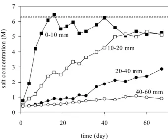
The changes in salt concentration with time at different depths in the soil are given in Fig. 4. The critical level of a salt-saturated solution was achieved after about 16 and 55 days at depths of 0–10 and 10–20 mm, respectively. After this time, the salt concentration was close to the critical level,
c. 6 M, which is the saturation concentration of NaCl at
25oC (Robinson and Stokes, 1959, p.476).
The accuracy of the method also depends on the
0 5 10 15 20 25 30 35 40 0 0.1 0.2 0.3 0.4
salt c onc entration (M)
el ec tr ic al c o nd u cti vi ty ( d S m -1)
Fig. 2. Calibration of a typical switch position of a four-electrode
salinity probe before (z) and after () the experiments. The continuous and dashed lines represent the regression equations
before and after the experiments, respectively.
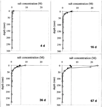
accumulated became very dry. Therefore, salt concentration in the solution increased further while the water content decreased, exceeding the limit of solubility so that salt precipitated. Figure 3 shows the results from gravimetric sampling and the salinity probes at four different times during the experiment. Salt concentration measured by the salinity probes was as accurate as the destructive method when the salt concentration in solution did not exceed maximum solubility. However, the probe did not respond to solid precipitated salt. Regression analyses between the
Fig. 3. Salt concentration in soil water against depth determined by
four-electrode probes (z) and destructive sampling () at different times. The dotted line represents the saturated concentration.
volumetric water content estimated at the same depth from the thermal-conductivity probes, and the other parameters and assumptions in the model of Rhoades et al. (1989). Our results suggested that the latter was adequate when applied to our weakly-structured sandy loam soil.
The probes were also used for 218 days after this experiment and proved quite durable after being used for a total of 285 days. However, some of the switches in the second probe (11, 12, 13, 14, 22, 23 and 24) failed on day 173 and salinity could not be monitored at these depths thereafter. This was probably because of disconnection between the electrical leads and the electrodes. Although stainless steel rings were used as electrodes, some corrosion was evident on some electrodes. The electrodes were cleaned after each experiment and the comparison of the results with the gravimetric method shows that this did not affect the measurements.
THERMAL CONDUCTIVITY PROBES
Eighteen probes were calibrated simultaneously with non-saline (pure) water and at constant temperature (18°C) before the experiment.
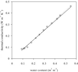
There is a linear relationship between volumetric water content, θ , and thermal conductivity, K, obtained from Eqn. (11). The general form of the thermal conductivity, K, versus water content, θ, curve is S-shaped (Hillel, 1980). However, Fig. 5 demonstrates a linear relationship between K and θ for Rivington soil over the range 0.10 < θ < 0.55 m3m–3. This relation cannot be used with other soil types or different ranges of water content. Similar linear relations between
thermal conductivity and water content have been obtained for silty loam soils by Al Nakshabandi and Kohnke (1964) and by Camillo and Gurney (1986).
Differences between individual probes were small, the coefficient of variation averaging 1.7% for all 13 calibration points, but decreasing as the soil dried, from 2.2% for the four wettest points to only 0.2% for the four driest (Fig.5). Statistical analyses showed that there were no significant differences between the probes at the 95% confidence level so that a single calibration line could be produced between thermal conductivity and water content. The linear relationship was K = a + bθ , with a = –0.0010 ± 0.0093,
b = 0.824 ± 0.031, and r = 0.993. However, an inverse
relation, such that
b a K− =
θ , was used to infer q from measurements of K estimated from Eqn. (11). This calibration line, produced before the experiment at 18°C and with pure water, was compared to those produced after the experiment and under different conditions (of salinity and temperature) to test the reproducibility and the variability of the calibration.
To test the reproducibility of the calibration, the probes were recalibrated at the same external temperature (18°C) after being used in the flow experiment for a period of 67 days. Figure 5 shows the calibration lines of the thermal conductivity probes before and after the experiment. There was no significant change (a = –0.0049 ± 0.0110,
b = 0.832 ± 0.034 and r = 0.990) from the original
calibration.
The temperature dependence of the sensors was tested by calibrating them at two different temperatures, at 18 and at
Fig. 4. Salt concentrations in soil water monitored by the
four-electrode probes as functions of time at different depths.
0 1 2 3 4 5 6 7 0 20 40 60 time (day) sa lt c o nc en tr at io n ( M ) 0-10 mm 10-20 mm 20-40 mm 40-60 mm
Fig. 5. Calibration of the thermal-conductivity probes at 18oC
before (z) and after () the experiments. The continuous and dashed lines represent the regression equations before and after the experiments, respectively. 0 0.1 0.2 0.3 0.4 0.5 0 0.1 0.2 0.3 0.4 0.5 0.6 water content (m3 m-3) th er m al c ond uc tivi ty ( W m -1 K -1 )
F. Konukcu, J.W. Gowing and D.A. Rose
38°C (a = –0.0022 ± 0.0085, b = 0.853 ± 0.028 and
r = 0.994) (Fig. 6). Although there was no statistically
significant difference between the lines, there was a small displacement of the calibration towards greater K values when measured at 38°C from those measured at 18°C.
To test the variability of the calibration under saline conditions, the probes were also calibrated with soil which was initially saturated with saline solution (0.274 M = 25 dS m–1). In this calibration, salts accumulated only in the top 20 mm when soil dried by evaporation. Because the
probes were placed 25 mm deep, the effect of the salinity in dry soil could not be investigated. However, Fig. 7 indicates that the measurements were unaffected by salinity in moist conditions (a = –0.0077 ± 0.0048, b = 0.858 ± 0.016 and
r = 0.998). There was no statistically significant difference
between the regression lines at the 95% confidence level. All values of a were not significantly different from zero.
The effect of the salinity in dry soil was well tested in the flow experiments conducted in the evaporation chamber. To test the performance of the probes, moisture contents measured using thermal conductivity probes are compared to the gravimetric method in Fig. 8. The measurements cover the entire range, from saturation to 0.10 m3 m–3, with great sensitivity and are unaffected by salt accumulation at the soil surface. In other experiments, the minimum water content obtained was c. 0.06 m3 m–3 and was measured successfully by the probes.
Although the probes were used over a period of 285 days, they were quite durable. However, two of them, placed close to the saturated zone, failed because of the deformation of the plastic tube used as a cover.
In this method, moisture measurements are based on generating heat. This causes moisture movement, particularly as vapour, away from the source of heat and
0 0.1 0.2 0.3 0.4 0.5 0 0.1 0.2 0.3 0.4 0.5 0.6 water co ntent (m3 m-3) the rm al c ond uc tivi ty (W m -1 K -1 )
Fig. 6. Calibration of the thermal-conductivity probes at 38oC().
The continuous and dashed lines represent the regression equations at 18oC and 38oC, respectively.
Fig. 7. Calibration of the thermal-conductivity probes with saline
() water at 18oC. The continuous and dashed lines represent the
regression equations with pure and saline water, respectively.
0 0.1 0.2 0.3 0.4 0.5 0 0.1 0.2 0.3 0.4 0.5 0.6 water co ntent (m3 m-3) th er m al c ond uc tivi ty ( W m -1 K -1 )
Fig. 8. Volumetric water content of the soil profile determined by
thermal-conductivity probes (z) and destructive sampling () at different times. 0 50 100 150 200 250 300 0 0.2 0.4 0.6 water content (m3 m-3) depth (mm) 4 d 0 50 100 150 200 250 300 0 0.2 0.4 0.6 water content (m3 m-3) depth (mm) 36 d 0 50 100 150 200 250 300 0 0.2 0.4 0.6 water content (m3 m-3) depth (mm) 16 d 0 50 100 150 200 250 300 0 0.2 0.4 0.6 water content (m3 m-3) depth (mm) 67 d
the amount of movement depends on both the temperature of the heat source and the length of time the heat is applied (Bloodworth and Page, 1975). In this study, the amount of heat produced, q, caused a maximum temperature difference of 1.7 K between the source and the soil during a period of 5 minutes, which was considered negligible.
Conclusions
The performance of the instruments in monitoring the distribution of soil water and salinity is very good, providing fine spatial resolution and continuous non-destructive measurements. Unlike other widely used methods (gypsum blocks, tensiometers), thermal-conductivity probes measured water content over the entire range from saturation to 0.06 m3 m–3 with great sensitivity and were unaffected by salt accumulation. The multi-electrode resisitivity probes provided reliable measurement of the salinity of the soil solution, but did not detect accumulation of salt in the solid phase (i.e. precipitation).
Both methods are rapid, simple and cheap, and probes can be manufactured and adapted easily to a variety of experimental situations. Both types of probe are quite stable during extended use, showing little if any drift from the original calibration curves. A single calibration curve can be used for the thermal-conductivity probes but, for the salinity probes, a specific cell constant must be determined for each group of four electrodes.
The thermal-conductivity probes also record the soil temperature simultaneously with the water content, both of which are required to estimate the electrical conductivity of the soil solution (Ew) from the soil bulk electrical conductivity (Ea). Hence, using thermal-conductivity and four-electrode salinity probes simultaneously for salinity research has great advantages over other techniques.
The thermal-conductivity probes can also be used to detect wetting and drying fronts accurately from direct measurement of water-content profiles because the probes are small in size and provide fine spatial resolution.
Acknowledgements
The authors thank technicians, D. McCallum (four-electrode probes) and K. Taylor (thermal-conductivity probes), for the construction of the instruments.
References
Al Nakshabandi, G. and Kohnke, H., 1964. Thermal conductivity and diffusivity of soils as related to moisture tension and other physical properties. Agric. Meteorol., 2, 271–279.
American Public Health Association, 1985. Standard Method for
Water and Waste Water Examination, 16th edition. WPCF,
AWWA.
Bloodworth, M.E. and Page, J.B., 1975. Use of thermistors for the measurement of soil moisture and temperature. Soil Sci.
Soc. Amer. Proc., 21, 11–15.
Bristow, K.L., Kluitenberg, G.J. and Horton, R., 1994a. Measurement of soil thermal properties with a dual-probe heat-pulse technique. Soil Sci. Soc. Amer. J., 58, 1288–1294. Bristow, K.L., White, R.D. and Kluitenberg, G.J., 1994b.
Comparison of single and dual probes for measuring soil thermal properties with transient heating. Aust. J. Soil. Res., 32, 447– 464
Camillo, P.J. and Gurney, R.J., 1986. A resistance parameter for bare-soil evaporation models. Soil Sci., 141, 95–105. Fritton, D.D., Busscher, W.J. and Alpert, J.E., 1974. An
inexpensive but durable thermal conductivity probe for field use. Soil Sci. Soc. Amer. Proc., 38, 854–855.
Fredlund, D.G., 1992. Background, theory, and research related to the use of thermal conductivity sensors for matric suction measurement. In: Advances in Measurement of Soil Physical
Properties: Bringing Theory into Practice, G.C.Topp,
W.D.Reynolds and R.E.Green (Eds.), Soil Science Society of America, Madison, WI, Special Publication No. 30, 249–261. Hillel, D., 1980. Fundamentals of Soil Physics. Academic Press,
London.
Jackson, R.D. and Taylor, S.A., 1986. Thermal conductivity and diffusivity. In: Methods of Soil Analysis: Part I, Physical and
Mineralogical Methods, A.Klute (Ed.) (2nd Edition), American
Society of Agronomy, Madison, WI, 945–956.
Nadler, A. and Frenkel, H., 1980. Determination of soil solution electrical conductivity from bulk soil electrical conductivity measurements by the four-electrode method. Soil Sci. Soc. Amer.
J., 44, 1216–1221.
Phene, C.J., Clarck, D.A., Cardon, G.E. and Mead, R.M., 1992. Soil matric potential sensor research and applications. In:
Advances in Measurements of Soil Physical Properties: Bringing Theory into Practice, G.C.Topp, W.D.Reynolds and R.E.Green
(Eds.). Soil Science Society of America, Madison, WI, Special
Publication No. 30, 263–280.
Rhoades, J.D., 1990. Sensing soil salinity: new technology. In:
Proc. 3rd National Irrigation Symposium, R.L.Elliott (Ed.),
Irrigation Association and ASCE, 28 Oct–1 Nov.1990, Phoenix, AZ, 422–428.
Rhoades, J.D., 1992. Instrumental field methods of salinity appraisal. In: Advances in Measurement of Soil Physical
Properties: Bringing Theory into Practice, G.C.Topp,
W.D.Reynolds and R.E.Green (Eds.). Soil Science Society of America, Madison, WI, Special Publication No. 30, 231–248. Rhoades, J.D., Raats, P.A.C. and Prather, R.J., 1976. Effects of liquid-phase electrical conductivity, water content, and surface conductivity on bulk soil electrical conductivity. Soil Sci. Soc.
Amer. J., 40, 651–655.
Rhoades, J.D., Manteghi, N.A., Shouse, P.J. and Alves, W.A., 1989. Soil electrical conductivity and soil salinity: new formulations and calibrations. Soil Sci. Soc. Amer. J., 53, 433– 439.
Robinson, R.A. and Stokes, R.H., 1959. Electrolyte Solutions (2nd edition), Butterworths, London.
Shainberg, I., Rhoades, J.D. and Prather, R.J., 1980. Effect of exchangeable sodium percentage, cation exchange capacity, and soil solution concentration on soil electrical conductivity. Soil
Sci. Soc. Amer. J., 44, 469–473.
Wechsler, A.E., Glaser, P.E. and McConnel, K.R., 1965. Methods
of laboratory and field measurements of thermal conductivity of soils. Cold Regions Research and Engineering Laboratory,