EUROPEAN ORGANISATION FOR NUCLEAR RESEARCH (CERN)
Phys. Rev. D92, 092004 (2015) DOI:10.1103/PhysRevD.92.092004
CERN-PH-EP-2015-225 12th November 2015
Searches for Higgs boson pair production in the
hh → bbττ, γγWW
∗, γγbb, bbbb channels with the ATLAS
detector
The ATLAS Collaboration
Abstract
Searches for both resonant and nonresonant Higgs boson pair production are performed in the hh → bbττ, γγWW∗ final states using 20.3 fb−1 of pp collision data at a center-of-mass energy of 8 TeV recorded with the ATLAS detector at the Large Hadron Collider. No evid-ence of their production is observed and 95% confidevid-ence-level upper limits on the produc-tion cross secproduc-tions are set. These results are then combined with the published results of the hh →γγbb, bbbb analyses. An upper limit of 0.69 (0.47) pb on the nonresonant hh produc-tion is observed (expected), corresponding to 70 (48) times the SM gg → hh cross secproduc-tion. For production via narrow resonances, cross-section limits of hh production from a heavy Higgs boson decay are set as a function of the heavy Higgs boson mass. The observed (ex-pected) limits range from 2.1 (1.1) pb at 260 GeV to 0.011 (0.018) pb at 1000 GeV. These results are interpreted in the context of two simplified scenarios of the Minimal Supersym-metric Standard Model.
c
2015 CERN for the benefit of the ATLAS Collaboration.
Reproduction of this article or parts of it is allowed as specified in the CC-BY-3.0 license.
1 Introduction
The Higgs boson discovered at the LHC in 2012 [1,2] opens a window for testing the scalar sector of the Standard Model (SM) and its possible extensions. Since the discovery, significant progress has been made in measuring its coupling strengths to fermions and vector bosons [3–6] as well as in studying its spin and its charge-conjugate and parity (CP) properties [7,8]. All results are consistent with those expected for the SM Higgs boson (here denoted by h). Within the SM, the existence of the Higgs boson is a consequence of the electroweak symmetry breaking (EWSB). This also predicts self-coupling between Higgs bosons, the measurement of which is crucial in testing the mechanism of EWSB. The self-coupling is one mechanism for Higgs boson pair production as shown in Fig.1(a). Higgs boson pairs can also be produced through other interactions such as the Higgs–fermion Yukawa interactions (Fig. 1(b)) in the Standard Model. These processes are collectively referred to as nonresonant production in this paper.
t/b h⇤ g g h h (a) t/b g g h h (b)
Figure 1: Leading-order Feynman diagrams of the nonresonant production of Higgs boson pairs in the Standard Model through (a) the Higgs boson self-coupling and (b) the Higgs–fermion Yukawa interactions.
Higgs boson pair production at the LHC as a probe of the self-coupling has been extensively studied in the literature [9–13]. One conclusion [14] is that the data collected so far (approximately 25 fb−1in total) are insensitive to the self-coupling in the SM, because of the expected small signal rates [15–17] and large backgrounds. However, it is essential to quantify the sensitivity of the current dataset and to develop tools for future measurements. Moreover, physics beyond the Standard Model (BSM) can potentially enhance the production rate and alter the event kinematics. For example, in the Minimal Supersymmetric Standard Model (MSSM) [18], a heavy CP-even neutral Higgs boson H can decay to a pair of lighter Higgs bosons. Production of H followed by its decay H → hh would lead to a new resonant process of Higgs boson pair production, in contrast to the nonresonant hh production predicted by the SM (Fig.1). In composite Higgs models such as those discussed in Refs. [19,20], increased production of nonresonant Higgs boson pairs is also expected.
Both the ATLAS and CMS collaborations have searched for nonresonant and/or resonant Higgs boson pair production [21–23]. In particular, ATLAS has published the results of searches in the hh → γγbb [21] and hh → bbbb [22] decay channels.1 In this paper, searches in two additional hh decay final states, bbττ and γγWW∗, are reported. For the hh → bbττ analysis, one tau lepton is required to decay to an
electron or a muon, collectively referred to as `, and the other tau lepton decays to hadrons (τhad). For
hh →γγWW∗, the h → WW∗→`νqq0 decay signature is considered in this study. The results of these new analyses are combined with the published results of hh → γγbb and hh → bbbb for both nonresonant and resonant production. The resonance mass mH considered in this paper ranges from 260 GeV to
1000 GeV. The lower bound is dictated by the 2mhthreshold while the upper bound is set by the search
range of the hh → bbττ analysis. The light Higgs boson mass mh is assumed to be 125.4 GeV, the
central value of the ATLAS measurement [24]. At this mass value, the SM predictions [25–27] for the decay fractions of hh → bbbb, bbττ, bbγγ and γγWW∗are, respectively, 32.6%, 7.1%, 0.26% and 0.10%. The resonant search assumes that gluon fusion is the production mechanism for a heavy Higgs boson that can subsequently decay to a pair of lighter Higgs bosons, i.e., gg → H → hh. Furthermore, the heavy Higgs boson is assumed to have a width significantly smaller than the detector resolution, which is approximately 1.5% in the best case (the hh → γγbb analysis). The potential interference between nonresonant and resonant production is ignored.
This paper is organized as follows. For the hh → bbττ and hh → γγWW∗ analyses, data and Monte Carlo (MC) samples are described in Sec.2and the object reconstruction and identification are outlined in Sec.3. In Secs.4and5, the separately published hh → γγbb and hh → bbbb analyses are briefly sum-marized. The hh → bbττ and hh → γγWW∗analyses including event selection, background estimations and systematic uncertainties are presented in Secs.6and7, respectively. The statistical and combination procedure is described in Sec.8. The results of the hh → bbττ and hh → γγWW∗analyses, as well as their combinations with the published analyses are reported in Sec.9. The implications of the resonant search for two specific scenarios of the MSSM, hMSSM [28,29] and low-tb-high [30], are discussed in Sec.10. These scenarios make specific assumptions and/or choices of MSSM parameters to accommodate the observed Higgs boson. Finally, a summary is given in Sec.11.
2 Data and Monte Carlo samples
The data used in the searches were recorded in 2012 with the ATLAS detector at the Large Hadron Collider in proton–proton collisions at a center-of-mass energy of 8 TeV and correspond to an integrated luminosity of 20.3 fb−1. The ATLAS detector is described in detail in Ref. [31]. Only data recorded when all subdetector systems were properly functional are used.
Signal and background MC samples are simulated with various event generators, each interfaced to Py-thia v8.175 [32] for parton showers, hadronization and underlying-event simulation. Parton distribution functions (PDFs) CT10 [33] or CTEQ6L1 [34] for the proton are used depending on the generator in question. MSTW2008 [35] and NNPDF [36] PDFs are used to evaluate systematic uncertainties. Table1
gives a brief overview of the event generators, PDFs and cross sections used for the hh → bbττ and hh →γγWW∗analyses. All MC samples are passed through the ATLAS detector simulation program [37]
based on GEANT4 [38].
Signal samples for both nonresonant and resonant Higgs boson pair production are generated using the leading-order MadGraph5 v1.5.14 [39] program. The nonresonant production is modeled using the SM DiHiggs model [40, 41] while the resonant production is realized using the HeavyScalar model [42], both implemented in MadGraph5. The heavy scalar H is assumed to have a narrow decay width of 10 MeV, much smaller than the experimental resolution. The SM prediction for the nonresonant gg → hh production cross section is 9.9 ± 1.3 fb [17] with mh= 125.4 GeV from the next-to-next-to-leading-order
calculation in QCD.
Single SM Higgs boson production is considered as a background. The Powheg r1655 generator [43–
45] is used to produce gluon fusion (ggF) and vector-boson fusion (VBF) events. This generator calcu-lates QCD corrections up to next-to-leading order (NLO), including finite bottom- and top-quark mass
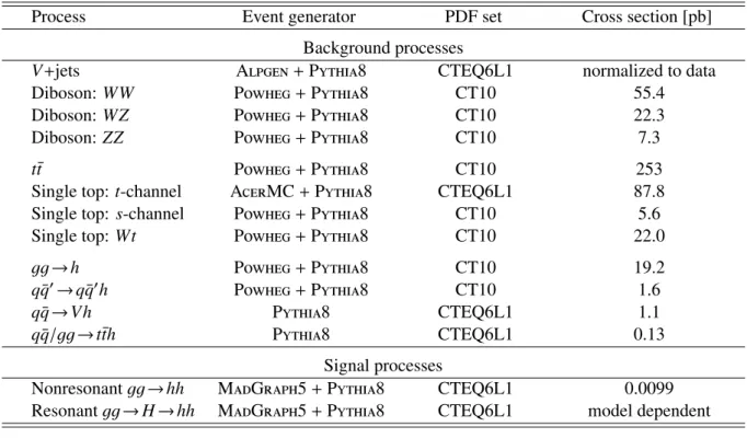
Table 1: List of MC generators and parton distribution functions of the signal and background processes used by the hh → bbττ and hh → γγWW∗analyses. SM cross sections used for the normalization are also given. For the WZ
and ZZ processes, contributions from γ∗are included and the cross sections quoted are for m
Z/γ∗> 20 GeV.
Process Event generator PDF set Cross section [pb]
Background processes
V+jets Alpgen + Pythia8 CTEQ6L1 normalized to data
Diboson: WW Powheg + Pythia8 CT10 55.4
Diboson: WZ Powheg + Pythia8 CT10 22.3
Diboson: ZZ Powheg + Pythia8 CT10 7.3
t¯t Powheg + Pythia8 CT10 253
Single top: t-channel AcerMC + Pythia8 CTEQ6L1 87.8
Single top: s-channel Powheg + Pythia8 CT10 5.6
Single top: Wt Powheg + Pythia8 CT10 22.0
gg→h Powheg + Pythia8 CT10 19.2
q¯q0→ q ¯q0h Powheg + Pythia8 CT10 1.6
q¯q → Vh Pythia8 CTEQ6L1 1.1
q¯q/gg → t¯th Pythia8 CTEQ6L1 0.13
Signal processes
Nonresonant gg → hh MadGraph5 + Pythia8 CTEQ6L1 0.0099
Resonant gg → H → hh MadGraph5 + Pythia8 CTEQ6L1 model dependent
effects [46]. The Higgs boson transverse momentum (pT) spectrum of the ggF process is matched to
the calculated spectrum at next-to-next-to-leading order (NNLO) and next-to-next-to-leading logarithm (NNLL) [47] in QCD corrections. Events of associated production q ¯q → Vh (here V = W or Z) and q¯q/gg → t¯th are produced using the Pythia8 generator [32]. All of these backgrounds are normalized using the state-of-the-art theoretical cross sections (see Table1) and their uncertainties compiled in Refs. [25–
27].
The Alpgen v2.1.4 program [48] is used to produce the V+jets samples. The Powheg generator is used to simulate top quark pair production (t¯t) as well as the s-channel and Wt processes of single top production; the t-channel process of single top production is simulated using the AcerMC v38 program [49]. The t¯t cross section has been calculated up to NNLO and NNLL in QCD corrections [50]. Cross sections for the three single-top processes have been calculated at (approximate) NNLO accuracy [51–53]. The Powheg generator is used to simulate diboson backgrounds (WW, WZ and ZZ). The diboson production cross sections are calculated at NLO in QCD corrections using the MCFM program [54,55].
3 Object identification
In this section, object reconstruction and identification for the hh → bbττ and hh → γγWW∗ analyses are discussed. The hh → bbττ and hh → γγWW∗ analyses are developed following the h → ττ [6] and h →γγ [56] studies of single Higgs bosons, respectively, and use much of their methodology.
Electrons are reconstructed from energy clusters in the electromagnetic calorimeter matched to tracks in the inner tracker. The calorimeter shower profiles of electron candidates must be consistent with those expected from electromagnetic interactions. Electron candidates are identified using tight and medium criteria [57] for the hh → bbττ and hh → γγWW∗ analyses, respectively. The selected candidates are required to have transverse momenta2 pT > 15 GeV and be within the detector fiducial volume of |η| <
2.47 excluding 1.37 < |η| < 1.52, the transition region between the barrel and endcap calorimeters. Muons are identified by matching tracks or segments reconstructed in the muon spectrometer with tracks reconstructed in the inner tracker. They are required to have pT > 10 GeV and |η| < 2.5. Both the
electrons and muons must satisfy calorimeter and track isolation requirements. The calorimeter isolation requires that the energy deposited in the calorimeter in a cone of size∆R ≡ p(∆η)2+ (∆φ)2= 0.2 around
the lepton (electron or muon), excluding the energy deposited by the lepton itself, is less than 6% (20%) of the pTof the lepton for the hh → bbττ (hh → γγWW∗) analysis. The track isolation is defined similarly:
the scalar pTsum of additional tracks originating from the primary vertex with pT > 1 GeV in a cone of
size∆R = 0.4 around the lepton is required to be less than 6% (15%) of the pTof the lepton track for the
hh → bbττ (hh→γγWW∗) analysis.
Photons are reconstructed from energy clusters in the electromagnetic calorimeter with their shower pro-files consistent with electromagnetic showers. A significant fraction of photons convert into e+e− pairs inside the inner tracker. Thus photon candidates are divided into unconverted and converted categories. Clusters without matching tracks are considered as unconverted photons, while clusters matched to tracks consistent with conversions are considered as converted photons. Photon candidates must fulfill the tight identification criteria [58] and are required to have pT> 25 GeV and |η| < 2.37 (excluding the transition
region 1.37 < |η| < 1.52) and must satisfy both calorimeter and track isolation. The calorimeter isolation requires the additional energy in a cone of∆R = 0.4 around the photon candidate to be less than 6 GeV while the track isolation requires the scalar pTsum of additional tracks in a cone of∆R = 0.2 around the
photon to be less than 2.6 GeV.
Jets are reconstructed using the anti-kt algorithm [59] with a radius parameter of R= 0.4. Their energies
are corrected for the average contributions from pileup interactions. Jets are required to have pT> 30 GeV
and |η| < 4.5. For the hh → γγWW∗analysis, a lower pT requirement of 25 GeV is applied for jets in the
central region of |η| < 2.4. To suppress contributions from pileup interactions, jets with pT < 50 GeV and
within the acceptance of the inner tracker (|η| < 2.4) must have over 50% of the scalar sum of the pT of
their associated tracks contributed by those originating from the primary vertex. Jets containing b-hadrons are identified using a multivariate algorithm (b-tagging) [60]. The algorithm combines information such as the explicit reconstruction of the secondary decay vertices and track impact-parameter significances. The operating point chosen for both hh → bbττ and hh → γγWW∗analyses has an efficiency of 80% for the b-quark jets in t¯t events.
Hadronically decaying τ candidates (τhad) are reconstructed using clusters in the electromagnetic and
hadronic calorimeters [61]. The tau candidates are required to have pT > 20 GeV and |η| < 2.5. The
number of tracks with pT > 1 GeV associated with the candidates must be one or three and the total
charge determined from these tracks must be ±1. The tau identification uses calorimeter cluster as well as tracking-based variables, combined using a boosted-decision-tree method [61]. Three working points,
2ATLAS uses a right-hand coordinate system with the interaction point as its origin and the beam line as its z-axis. The x-axis points to the center of the LHC ring and y-axis points upwards. The pseudorapidity η is defined as η= − ln tan(θ/2), where θ is the polar angle measured with respect to the z-axis. The transverse momentum pTis calculated from the momentum p: pT= p sin θ.
labeled loose, medium and tight [61], corresponding to different identification efficiencies are used. Ded-icated algorithms that suppress electrons and muons misidentified as τhadcandidates are applied as well.
The missing transverse momentum (with magnitude ETmiss) is the negative of the vector sum of the trans-verse momenta of all photon, electron, muon, τhad, and jet candidates, as well as the pT of all
calori-meter clusters not associated with these reconstructed objects, called the soft-term contribution [62]. The hh → bbττ analysis uses the version of the Emiss
T calculation in the h → ττ analysis [6]. In this calculation,
the soft-term contribution is scaled by a vertex fraction, defined as the ratio of the summed scalar pT of
all tracks from the primary vertex not matched with the reconstructed objects to the summed scalar pT
of all tracks in the event. The hh → γγWW∗analysis, on the other hand, uses the EmissT -significance em-ployed by the h → γγ study [56]. It is defined as the ratio of the measured EmissT to its expected resolution estimated using the square root of the scalar sum of the transverse energies of all objects contributing to the EmissT calculation.
4 Summary of hh →
γγbb
The hh → γγbb analysis, published in Ref. [21], largely follows the ATLAS analysis of the Higgs boson discovery in the h → γγ decay channel [1, 56]. The search is performed in the √s = 8 TeV dataset corresponding to an integrated luminosity of 20.3 fb−1. The data were recorded with diphoton triggers that are nearly 100% efficient for events satisfying the photon requirements. Events must contain two isolated photons. The pT for the leading (subleading) photon must be larger than 35% (25%) of the
diphoton invariant mass mγγ, which itself must be in the range of 105 < mγγ < 160 GeV. Events must
also contain two energetic b-tagged jets; the leading (subleading) jet must have pT > 55 (35) GeV, and
the dijet mass must fall within a window 95 < mbb < 135 GeV, as expected from the h → bb decay. A
multivariate b-tagging algorithm [60] that is 70% efficient for the b-quark jets in t¯t events is applied. Backgrounds for both the resonant and nonresonant analyses are divided into two categories: events con-taining a single real Higgs boson (with h → γγ), and the continuum background of events not concon-taining a Higgs boson. The former are evaluated purely from simulation, and are small compared to the continuum background, which is evaluated from data in the diphoton mass sidebands (the mγγrange of 105–160 GeV excluding the region of mh± 5 GeV). In the nonresonant analysis, an unbinned signal-plus-background fit
is performed on the observed mγγdistribution, with the background from single Higgs bosons constrained to the expectation from the SM. The continuum background is modeled with an exponential function; the shape of the exponential function is taken from data containing a diphoton and dijet pair where fewer than two jets are b-tagged.
The resonant search proceeds in a similar manner, although it is ultimately a counting experiment, with an additional requirement on the four-object invariant mass mγγbb, calculated with the bb mass constrained to mh. This requirement on mγγbbvaries with the resonance mass hypothesis under evaluation, and is defined
as the smallest window containing 95% of the signal events based on MC simulation. As in the nonres-onant search, the number of background events with real Higgs bosons is estimated from simulation. The continuum background in the mγγsignal window is extrapolated from the diphoton mass sidebands. A resonance with mass between 260 GeV and 500 GeV is considered in the search.
The small number of events (nine) in the diphoton mass sideband leads to large statistical uncertainties (33%) on the dominant continuum background, so that most systematic uncertainties have a small effect on the final result. For the resonant search, however, systematic uncertainties with comparable effect
remain. Uncertainties of 0–30% (depending on the resonance mass hypothesis under consideration) are assigned due to the modeling of the mγγbbshape using the data with less than two b-tagged jets. Additional uncertainties of 16–30% arise from the choice of functional form used to parameterize the shape of mγγbb.
In the nonresonant analysis, extrapolating the sidebands into the diphoton mass window of the signal selection leads to a prediction of 1.3 continuum background events. An additional contribution of 0.2 events is predicted from single Higgs boson production. A total of five events are observed, representing an excess of 2.4 standard deviations (σ). A 95% confidence level (CL) upper limit of 2.2 (1.0) pb is observed (expected) for σ(gg → hh), the cross section of nonresonant Higgs boson pair production. For the resonant searches, the observed (expected) upper limits on σ(gg → H) × BR(H → hh) are 2.3 (1.7) pb at mH= 260 GeV and 0.7 (0.7) pb at mH= 500 GeV.
5 Summary of hh → bbbb
The hh → bbbb analysis [22] benefits from the large branching ratio of h → bb. The analysis employs resolved as well as boosted Higgs boson reconstruction methods. The resolved method attempts to re-construct and identify separate b-quark jets from the h → bb decay, while the boosted method uses a jet substructure technique to identify the h → bb decay reconstructed as a single jet. The latter is expected if the Higgs boson h has a high momentum. The boosted method is particularly suited to the search for a resonance with mass above approximately 1000 GeV decaying to a pair of SM Higgs bosons. For the combinations presented in this paper, resonances below this mass are considered and the resolved method is used as it is more sensitive.
The analysis with the resolved method searches for two back-to-back and high-momentum bb systems with their masses consistent with mhin a dataset at
√
s= 8 TeV corresponding to an integrated luminosity of 19.5 fb−1for the triggers used. The data were recorded with a combination of multijet triggers using information including the b-quark jet tagging. The trigger is > 99.5% efficient for signal events satisfying the offline selection. Candidate events are required to have at least four b-tagged jets, each with pT >
40 GeV. As in the hh → γγbb analysis, a multivariate b-tagging algorithm [60] with an estimated efficiency
of 70% is used to tag jets containing b-hadrons. The four highest-pTb-tagged jets are then used to form
two dijet systems, requiring the angular separation∆R in (η, φ) space between the two jets in each of the two dijet systems to be smaller than 1.5. The transverse momenta of the leading and subleading dijet systems must be greater than 200 GeV and 150 GeV, respectively. These selection criteria, driven partly by the corresponding jet trigger thresholds and partly by the necessity to suppress the backgrounds, lead to significant loss of signal acceptance for lower resonance masses. The resonant search only considers masses above 500 GeV. The leading (m12) and subleading (m34) dijet invariant mass values are required
to be consistent with those expected for the hh → bbbb decay, satisfying the requirement:
v t m12− m012 σ12 2 + m34− m034 σ34 2 < 1.6. Here m0
12(124 GeV) and m034 (115 GeV) are the expected peak values from simulation for the leading
and subleading dijet pair, respectively, and σ12 and σ34 are the dijet mass resolutions, estimated from
the simulation to be 10% of the dijet mass values. More details about the selection can be found in Ref. [22].
After the full selection, more than 90% of the total background in the signal region is estimated to be multijet events, while the rest is mostly t¯t events. The Z+jets background constitutes less than 1% of the total background and is modeled using MC simulation. The multijet background is modeled using a fully data-driven approach in an independent control sample passing the same selection as the signal except that only one of the two selected dijets is b-tagged. This control sample is corrected for the kinematic differences arising from the additional b-tagging requirements in the signal sample. The t¯t contribution is taken from MC simulations normalized to data in dedicated control samples.
The dominant sources of systematic uncertainty in the analysis are the b-tagging calibration and the modeling of the multijet background. The degradation in the analysis sensitivity from these uncertainties is below 10%. Other sources of systematic uncertainty include the t¯t modeling, and the jet energy scale and resolution, which are all at the percent level. A total of 87 events are observed in the data, in good agreement with the SM expectation of 87.0 ± 5.6 events. Good agreement is also observed in the four-jet invariant mass distribution, thus there is no evidence of Higgs boson pair production. For the nonresonant search, both the observed and expected 95% CL upper limit on the cross section σ(pp → hh → bbbb) is 202 fb. For the resonant search, the invariant mass of the four jets is used as the final discriminant from which the upper limit on the potential signal cross section is extracted. The resulting observed (expected) 95% CL upper limit on σ(pp → H → hh → bbbb) ranges from 52 (56) fb, at mH= 500 GeV, to 3.6 (5.8) fb,
at mH= 1000 GeV.
6 hh → bbττ
This section describes the search for Higgs boson pair production in the hh → bbττ decay channel, where only the final state where one tau lepton decays hadronically and the other decays leptonically, bb`τhad,
is used. The data were recorded with triggers requiring at least one lepton with pT > 24 GeV. These
triggers are nearly 100% efficient for events passing the final selection. Candidate bb`τhad events are
selected by requiring exactly one lepton with pT > 26 GeV, one hadronically decaying tau lepton of the
opposite charge with pT > 20 GeV meeting the medium criteria [61], and two or more jets with pT >
30 GeV. In addition, between one and three of the selected jets must be b-tagged using the multivariate b-tagger. The upper bound on the number of b-tagged jets is designed to make this analysis statistically independent of the hh → bbbb analysis summarized in Sec.5. These criteria are collectively referred to as the “preselection”.
The backgrounds from W+jets, Z → ττ, diboson (WW, WZ and ZZ) and top quark (both t¯t and single top quark) production dominate the surviving sample and their contributions are derived from a mixture of data-driven methods and simulation. The contribution from events with a jet misidentified as a τhad,
referred to as the fake τhadbackground, are estimated using data with a “fake-factor” method. The method
estimates contributions from W+jets, multijet, Z+jets and top quark events that pass the event selection due to misidentified τhadcandidates. The fake factor is defined as the ratio of the number of τhadcandidates
identified as medium, to the number satisfying the loose, but not the medium, criteria [61]. The pT
-dependent fake factors are measured in data control samples separately for the τhadcandidates with one or
three tracks and for W+jets, multijet, Z+jets and top quark contributions. The W+jets, multijet, Z+jets and top quark control samples are selected by reversing the mT cut (see below), relaxing the lepton isolation
requirement, reversing the dilepton veto or by requiring b-tagged jets, respectively. The fake factors determined from these control samples are consistent within their statistical uncertainties. They are then applied to the signal control sample, i.e., events passing the selection, except that the τhad candidate is
required to satisfy the loose, but not the medium, τhadidentification, to estimate the fake τhadbackground.
The composition of the sample is determined from a mixture of data-driven methods and MC simulations and it is found that the sample is dominated by the W+jets and multijet events. Details of the method can be found in Ref. [61]. The method is validated using the same-sign `τhad events that are otherwise
selected in the same way as the signal candidates.
The Z → ττ background is modeled using selected Z → µµ events in data through embedding [63], where the muon tracks and associated energy depositions in the calorimeters are replaced by the corresponding simulated signatures of the final-state particles of tau decays. In this approach, the kinematics of the produced boson, the hadronic activity of the event (jets and underlying event) as well as pileup are taken from data [6]. Other processes passing the Z → µµ selection, primarily from top quark production, are subtracted from the embedded data sample using simulation. Their contributions are approximately 2% for events with one b-tagged jet and 25% for events with two or more b-tagged jets. The Z → ττ background derived is found to be in a good agreement with that obtained from the MC simulation. The remaining backgrounds, mostly t¯t and diboson events with genuine `τhadin their decay final states,
are estimated using simulation. The small contributions from single SM Higgs boson production and from Z(→ ee/µµ)+ jets events (in which one of the electrons or muons is misidentified as τhad) are also
estimated from simulation. The production rates of these processes are normalized to the theoretical cross sections discussed in Sec.2. For the simulation of the t¯t process, the top quark pTdistribution is corrected
for the observed difference between data and simulation [64]. The background from misidentified leptons is found to be negligible.
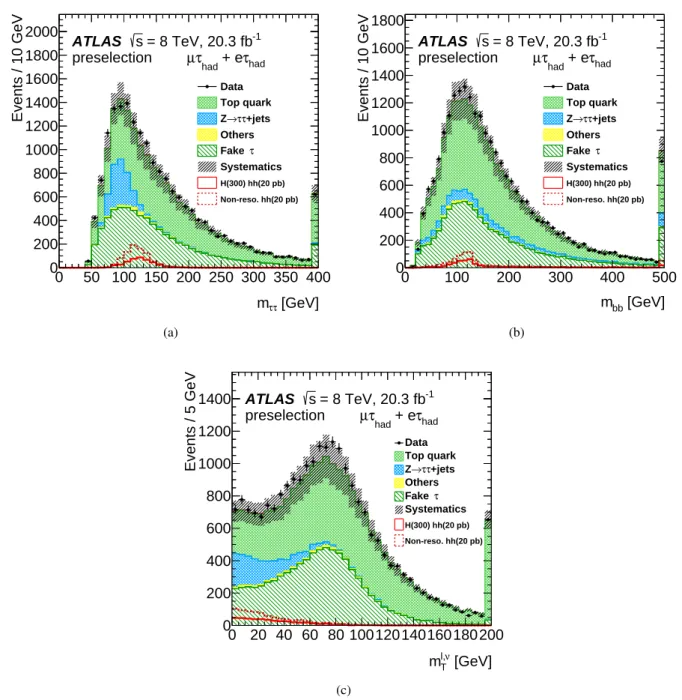
Figures 2(a) and 2(b) compare the observed ditau (mττ) and dijet (mbb) mass distributions with those
expected from background events after the preselection discussed above. The sample is dominated by contributions from top quark production, fake τhad, and Z → ττ backgrounds. Also shown in the figures are
the expected signal distributions for a Higgs boson pair production cross section of 20 pb as an illustration. The yield of the nonresonant production is significantly higher than that of the resonant production for the same cross section, largely due to the harder pT spectrum of the Higgs boson h of the nonresonant
production. The ditau invariant mass is reconstructed from the electron or muon, τhad, and EmissT using a
method known as the missing mass calculator (MMC) [65]. The MMC solves an underconstrained system of equations with solutions weighted by EmissT resolution and the tau-lepton decay topologies. It returns the most probable value of the ditau mass, assuming that the observed lepton, τhad and ETmissstem from a
ττ resonance. The dijet mass is calculated from the two leading b-tagged jets, or using also the highest-pT
untagged jet if only one jet is b-tagged.
Additional topological requirements are applied to reduce the background. As shown in Fig.2(c), the signal events tend to have small values of the transverse mass m`νT calculated from the lepton and ETmiss system. Consequently, a requirement of m`νT < 60 GeV is applied, which reduces the background signi-ficantly with only a small loss of the signal efficiency. In addition, the angular separation in the transverse plane between the ETmiss and τhad is required to be larger than one radian to reduce the fake τhad
back-ground.
Background events from t¯t → WWbb → `ντνbb decay have an identical visible final state to the signal if the tau lepton decays hadronically. For signal h → ττ → `τhad events, however, the pT of the lepton
tends to be softer than that of the τhad due to the presence of more neutrinos in the τ → ` decays. Thus
the pT of the electron or muon is required to satisfy pT(`) < pT(τhad)+ 20 GeV. The t¯t events of the
t¯t → WW bb →`ν qq0bbfinal state with a misidentified τhad candidate remain a large background. To
[GeV] τ τ m 0 50 100 150 200 250 300 350 400 Events / 10 GeV 0 200 400 600 800 1000 1200 1400 1600 1800 2000 -1 = 8 TeV, 20.3 fb s had τ + e had τ µ Data Top quark +jets τ τ → Z Others τ Fake Systematics H(300) hh(20 pb) Non-reso. hh(20 pb) ATLAS preselection (a) [GeV] bb m 0 100 200 300 400 500 Events / 10 GeV 0 200 400 600 800 1000 1200 1400 1600 1800 -1 = 8 TeV, 20.3 fb s had τ + e had τ µ Data Top quark +jets τ τ → Z Others τ Fake Systematics H(300) hh(20 pb) Non-reso. hh(20 pb) ATLAS preselection (b) [GeV] ν l, T m 0 20 40 60 80 100120140160180200 Events / 5 GeV 0 200 400 600 800 1000 1200 1400 s = 8 TeV, 20.3 fb-1 had τ + e had τ µ Data Top quark +jets τ τ → Z Others τ Fake Systematics H(300) hh(20 pb) Non-reso. hh(20 pb) ATLAS preselection (c)
Figure 2: Kinematic distributions of the hh → bbττ analysis after the preselection (see text) comparing data with the expected background contributions: (a) ditau mass mττ reconstructed using the MMC method, (b) dijet mass mbb
and (c) the transverse mass m`νT of the lepton and the EmissT system. The top quark background includes contributions from both t¯t and the single top-quark production. The background category labeled “Others” comprises diboson and Z → ee/µµ contributions. Contributions from single SM Higgs boson production are included in the background estimates, but are too small to be visible on these distributions. As illustrations, expected signal distributions for a Higgs boson pair production cross section of 20 pb are overlaid for both nonresonant and resonant Higgs boson pair production. A mass of mH= 300 GeV is assumed for the resonant production. The last bin in all distributions
represents overflows. The gray hatched bands represent the uncertainties on the total background contributions. These uncertainties are largely correlated from bin to bin.
untagged jet and its mass mτ jis calculated. The W candidate is then paired with a b-tagged jet to form
the top quark candidate with a reconstructed mass mτ jb. The pairing is chosen to minimize the mass sum m`b+ mτbfor events with two or more b-tagged jets. If only one jet is b-tagged, one of the b-jets in the mass sum is replaced by the highest-pTuntagged jet. An elliptical requirement in the form of a χ2in the
(mτ j, mτ jb) plane: ∆mWcos θ −∆mtsin θ 28 GeV !2 + ∆mWsin θ+ ∆mtcos θ 18 GeV !2 > 1
is applied to reject events with (mτ j, mτ jb) consistent with the hypothesis (mW, mt), the masses of the W
boson and the top quark. Here∆mW = mτ j− mW, ∆mt = mτ jb− mt and θ is a rotation angle given by
tan θ= mt/mW to take into account the average correlation between mτ jand mτ jb.
Finally, the remaining events must have 90 < mbb < 160 GeV, consistent with the expectation for the
h → bbdecay. For the nonresonant search, mττis used as the final discriminant to extract the signal, and
its distribution is shown in Fig.3(a). The selection efficiency for the gg → hh → bbττ signal is 0.57%.
For the resonant search, the MMC mass is required to be in the range of 100 < mττ < 150 GeV. The
mass resolutions of mbband mττare comparable for the signal, but the mbbdistribution has a longer tail.
The resonance mass mbbττ reconstructed from the dijet and ditau system is used as the discriminant. To improve the mass resolution of the heavy resonances, scale factors of mh/mbb and mh/mττ are applied
respectively to the four-momenta of the bb and ττ systems, where mh is set to the value of 125 GeV
used in the simulation. The resolution of mbbττ is found from simulation studies to vary from 2.4% at mH = 260 GeV to 4.8% at 1000 GeV. The improvement in the resolution from the rescaling is largest at
low mass and varies from approximately a factor of three at 260 GeV to about 30% at 1000 GeV. The reconstructed mbbττdistribution for events passing all the selections is shown in Fig.3(b). The efficiency
for the gg → H → hh → bbττ signal varies from 0.20% at 260 GeV to 1.5% at 1000 GeV. These efficiencies include branching ratios of the tau lepton decays, but not those of heavy or light Higgs bosons.
To take advantage of different signal-to-background ratios in different kinematic regions, the selected events are divided into four categories based on the ditau transverse momentum pττT (less than or greater than 100 GeV) and the number of b-tagged jets (nb = 1 or ≥ 2) for both the nonresonant and resonant
searches. The numbers of events expected from background processes and observed in the data passing the resonant hh → bbττ selection are summarized in Table2for each of the four categories. The expected number of events from the production of a Higgs boson with mH = 300 GeV and a cross section of
σ(gg→ H) × BR(H →hh) = 1 pb for each category is also shown for comparison.
Systematic uncertainties from the trigger, luminosity, object identification, background estimate as well as Monte Carlo modeling of signal and background processes are taken into account in the background estimates and the calculation of signal yields. The impact of these systematic uncertainties varies for different background components and event categories. For the most sensitive nb ≥ 2 categories, the main
background contributions are from top quark, fake τhad, and Z → ττ. The jet energy scale and resolution is
the largest uncertainty for the top-quark contribution, ranging between 10% and 19% for the nonresonant and resonant searches. The leading source of systematic uncertainty for the fake τhad background is the
“fake-factor” determination, due to the uncertainties of the sample composition. Varying the composition of W+jets, Z+jets, top quark and multijet events in the control samples by ±50% leads to a change in the estimated fake τhad background by 9.5%. The most important source of systematic uncertainty
for the Z → ττ background is the t¯t subtraction from the Z → µµ sample used for the embedding, due to the uncertainty on the t¯t normalization. Its effect ranges from 8% to 15%. The overall systematic uncertainties on the total background contributions to the high (low) pττT category of nb ≥ 2 are 12%
Table 2: The numbers of events predicted from background processes and observed in the data passing the final selection of the resonant search for the four categories. The top quark background includes contributions from both t¯tand the single top-quark production. The “others” background comprises diboson and Z → ee/µµ contributions. The numbers of events expected from the production of a mH = 300 GeV Higgs boson with a cross section of
σ(gg→ H)×BR(H →hh) = 1 pb are also shown as illustrations. The uncertainties shown are the total uncertainties, combining statistical and systematic components.
nb= 1 nb≥ 2
Process pττT < 100 GeV pττT > 100 GeV pττT < 100 GeV pττT > 100 GeV
SM Higgs 0.5 ± 0.1 0.8 ± 0.1 0.1 ± 0.1 0.2 ± 0.1 Top quark 30.3 ± 3.6 19.6 ± 2.5 30.9 ± 3.0 23.6 ± 2.5 Z →ττ 38.1 ± 4.4 20.2 ± 3.7 6.8 ± 1.8 2.6 ± 1.0 Fake τhad 37.0 ± 4.4 12.1 ± 1.7 13.7 ± 1.9 5.4 ± 1.0 Others 3.2 ± 3.7 0.5 ± 1.5 0.7 ± 1.6 0.2 ± 0.7 Total background 109.1 ± 8.6 53.1 ± 6.0 52.2 ± 8.2 32.1 ± 5.4 Data 92 46 35 35 Signal mH= 300 GeV 0.8 ± 0.2 0.4 ± 0.2 1.5 ± 0.3 0.9 ± 0.2 [GeV] τ τ m 0 100 200 300 400 500 Events / 25 GeV 0 20 40 60 80 100 120 140 160 180 200 220 Data Top quark +jets τ τ → Z Others τ Fake Systematics Non-reso. hh(10 pb) ATLAS s = 8 TeV, 20.3 fb-1 had τ + e had τ µ (a) [GeV] τ τ bb m 200 300 400 500 600 700 800 900 Events / 25 GeV 0 10 20 30 40 50 60 70 Data Top quark +jets τ τ → Z Others τ Fake Systematics H(300) hh(10 pb) ATLAS s = 8 TeV, 20.3 fb-1 had τ + e had τ µ (b)
Figure 3: Distributions of the final discriminants used to extract the signal: (a) mττfor the nonresonant search and
(b) mbbττfor the resonant search. The top quark background includes contributions from both t¯t and the single
top-quark production. The background category labeled “Others” comprises diboson and Z → ee/µµ contributions. Contributions from single SM Higgs boson production are included in the background estimates, but are too small to be visible on these distributions. As illustrations, the expected signal distributions assume a cross section of 10 pb for Higgs boson pair production for both the nonresonant and resonant searches. In (b), a resonance mass of 300 GeV is assumed. The gray hatched bands represent the uncertainties on the total backgrounds. These uncertainties are largely correlated from bin to bin.
from jet and tau energy scales and b-tagging. The modeling of top quark production is also an important systematic uncertainty for the category with two or more b-tagged jets and high pττT.
The uncertainties on the signal acceptances are estimated from experimental as well as theoretical sources. The total experimental systematic uncertainties vary between 12% and 24% for the categories with two or more b-tagged jets, and are dominated by the jet and tau energy scales and b-tagging. Theoretical uncertainties arise from the choice of parton distribution functions, the renormalization and factorization scales as well as the value of strong coupling constant αsused to generate the signal events. Uncertainties
of 3%, 1% and 3% from the three sources, respectively, are assigned to all signal acceptances.
For the nonresonant search, the observed ditau mass distribution agrees well with that of the estimated background events as shown in Fig.3(a). For the resonant search, a small deficit with a local significance of approximately 2σ is observed in the data relative to the background expectation at mbbττ ∼ 300 GeV as is shown in Fig.3(b). No evidence of Higgs boson pair production is present in the data. The resulting upper limits on Higgs boson pair production from these searches are described in Sec.9.
7 hh →
γγWW
∗This section describes the search for Higgs boson pair production in the hh → γγWW∗ decay channel, where one Higgs boson decays to a pair of photons and the other decays to a pair of W bosons. The h → γγ decay is well suited for tagging the Higgs boson. The small Higgs boson width together with the excellent detector resolution for the diphoton mass strongly suppresses background contributions. Moreover, the h → WW∗decay has the largest branching ratio after h → bb. To reduce multijet backgrounds, one of the Wbosons is required to decay to an electron or a muon (either directly or through a tau lepton) whereas the other is required to decay hadronically, leading to the γγ`νqq0final state.
The data used in this analysis were recorded with diphoton triggers with an efficiency close to 100% for diphoton events passing the final offline selection. The diphoton selection follows closely that of the ATLAS measurement of the h → γγ production rate [56] and that of the hh → γγbb analysis [21]. Events are required to have two or more identified photons with the leading and subleading photon candidates having pT/mγγ> 0.35 and 0.25, respectively, where mγγis the invariant mass of the two selected photons.
Only events with mγγin the range of 105 < mγγ< 160 GeV are considered.
Additional requirements are applied to identify the h → WW∗→`νqq0 decay signature. Events must have two or more jets, and exactly one lepton, satisfying the identification criteria described in Sec.3. To reduce multijet backgrounds, the events are required to have ETmisswith significance greater than one. Events with any b-tagged jet are vetoed to reduce contributions from top quark production.
A total of 13 events pass the above selection. The final hh → γγWW∗candidates are selected by requiring the diphoton mass mγγto be within a ±2σ window of the Higgs boson mass in h → γγ where σ is taken to be 1.7 GeV. Due to the small number of events, both nonresonant and resonant searches proceed as count-ing experiments. The selection efficiency for the hh → γγWW∗signal of SM nonresonant Higgs boson
pair production is estimated using simulation to be 2.9%. For the resonant production, the corresponding efficiency varies from 1.7% at 260 GeV to 3.3% at 500 GeV. These efficiencies include the branching ratios of the W boson decays, but not those of the Higgs boson decays.
The background contributions considered are single SM Higgs boson production (gluon fusion, vector-boson fusion and associated production of Wh, Zh and t¯th) and continuum backgrounds in the mγγ spec-trum. Events from single Higgs boson production can mimic the hh → γγWW∗signal if, for example, the Higgs boson decays to two photons and the rest of the event satisfies the h → WW∗→`νqq0identification. These events would exhibit a diphoton mass peak at mh. As in the hh → bbττ analysis, their contributions
are estimated from simulation using the SM cross sections [27]. The systematic uncertainty on the total yield of these backgrounds is estimated to be 29%, dominated by the modeling of jet production (27%). The total number of events expected from single SM Higgs production is therefore 0.25 ± 0.07 with con-tributions of 0.14, 0.08 and 0.025 events from Wh, t¯th and Zh processes, respectively. Concon-tributions from gluon and vector-boson fusion processes are negligible.
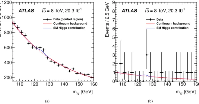
[GeV] γ γ m 110 120 130 140 150 160 Events / 2.5 GeV 200 400 600 800 1000 1200
Data (control region) Continuum background SM Higgs contribution -1 = 8 TeV, 20.3 fb s ATLAS (a) [GeV] γ γ m 110 120 130 140 150 160 Events / 2.5 GeV 0 1 2 3 4 5 6 7 8 9 Data Continuum background SM Higgs contribution -1 = 8 TeV, 20.3 fb s ATLAS (b)
Figure 4: The distribution of the diphoton invariant mass for events passing (a) the relaxed requirements and (b) the final selection. The relaxed requirements include all final selections except those on the lepton and ETmiss. The red curves represent the continuum background contributions and the blue curves include the contributions expected from single SM Higgs boson production estimated from simulation. The continuum background contributions in the signal mγγmass window are shown as dashed lines.
The background that is nonresonant in the γγ mass spectrum is measured using the continuum background in the mγγspectrum. The major source of these backgrounds is Wγγ+ jets events with a W → `ν decay. These events are expected to have a diphoton mass distribution with no resonant structure at mhand their
contribution (NSRest) in the signal region, mγγ∈ mh± 2σ, is estimated from the mγγsidebands in the data:
NSRest = NSBData× fSB 1 − fSB
.
Here NSBData is the number of events in the data sidebands, defined as the mass region 105 < mγγ <
160 GeV excluding the signal region. The quantity fSB is the fraction of background events in 105 <
mγγ < 160 GeV falling into the signal mass window, and can in principle be determined from a fit of
selection makes such a fit unsuitable. Instead, fSB is determined in a data control sample, selected as
the signal sample without the lepton and ETmiss requirements. Figure4(a) shows the mγγ distribution of events in the control sample. For the fit, an exponential function is used to model the sidebands and a wider region of mh± 5 GeV is excluded to minimize potential signal contamination in the sidebands. The
fit yields a value of fSB = 0.1348 ± 0.0001. Varying the fit range of the sidebands leads to negligible
changes. Different fit functions, such as a second-order polynomial or an exponentiated second-order polynomial, lead to a difference of 1.4% in fSB. To study the sample dependence of fSB, the fit is repeated
for the control sample without the jet and ETmiss requirements and a difference of only 2% is observed. Simulation studies show that the continuum background is dominated by W(`ν)γγ+ jets production. The γγ`ν +jets events generated using MadGraph reproduce well the observed mγγdistribution. The potential
difference between γγ+jets and γγ`ν+jets samples is studied using simulation. A difference below 1% is observed. Taking all these differences as systematic uncertainties, the fraction of background events in the signal mass window is fSB= 0.135 ± 0.004. With 9 (NSBData) events observed in the data sidebands, it leads
to NSRest = 1.40 ± 0.47 events from the continuum background. Figure4(a) also shows the contribution expected from single SM Higgs boson production. The data prefer a larger cross section than the SM prediction for single Higgs boson production, consistent with the measurement reported in Ref. [66]. The uncertainties on the signal acceptances are estimated following the same procedure as the hh → bbττ analysis. The total experimental uncertainty is found to vary between 4% and 7% for different signal samples under consideration, dominated by the contribution from the jet energy scale. The theoretical uncertainties from PDFs, the renormalization and factorization scales, and the strong coupling constant are 3%, 1%, and 3%, respectively, the same as for the hh → bbττ analysis.
The mγγ distribution of the selected events in the data is shown in Fig. 4(b). In total, 13 events are found with 105 < mγγ < 160 GeV. Among them, 4 events are in the signal mass window of mh± 2σ
compared with 1.65 ± 0.47 events expected from single SM Higgs boson production and continuum background processes. The p-value of the background-only hypothesis is 3.8%, corresponding to 1.8 standard deviations.
Assuming a cross section of 1 pb (σ(gg → hh) or σ(gg → H) × BR(H → hh)) for Higgs boson pair production, the expected number of signal events is 0.64 ± 0.05 for the nonresonant production. For the resonant production, the corresponding numbers of events are 0.47 ± 0.05 and 0.72 ± 0.06 for a resonance mass of 300 GeV and 500 GeV, respectively. The implications of the search for Higgs boson pair production are discussed in Sec.9.
8 Combination procedure
The statistical analysis of the searches is based on the framework described in Refs. [67–70]. Profile-likelihood-ratio test statistics are used to measure the compatibility of the background-only hypothesis with the observed data and to test the hypothesis of Higgs boson pair production with its cross section as the parameter of interest. Additional nuisance parameters are included to take into account systematic uncertainties and their correlations. The likelihood is the product of terms of the Poisson probability constructed from the final discriminant and of nuisance parameter constraints with either Gaussian, log-normal, or Poisson distributions. Upper limits on the Higgs boson pair production cross section are derived using the CLs method [71]. For the combinations, systematic uncertainties that affect two or
more analyses (such as those of luminosity, jet energy scale and resolutions, b-tagging, etc.) are modeled with common nuisance parameters.
For the hh → bbττ analysis, Poisson probability terms are calculated for the four categories separately from the mass distributions of the ditau system for the nonresonant search (Fig. 3(a)) and of the bbττ system for the resonant search (Fig.3(b)). The mbbττ distributions of the resonant search are rebinned to ensure a sufficient number of events for the background prediction in each bin, in particular a single bin is used for mbbττ & 400 GeV for each category. For the hh → γγWW∗ analysis, event yields are used to calculate Poisson probabilities without exploiting shape information. The hh → γγbb and hh → bbbb analyses are published separately in Refs. [21,22]. However, the results are quoted at slightly different values of the Higgs boson mass mh and, therefore, have been updated using a common mass value of
mh = 125.4 GeV [24] for the combinations. The decay branching ratios of the Higgs boson h and their
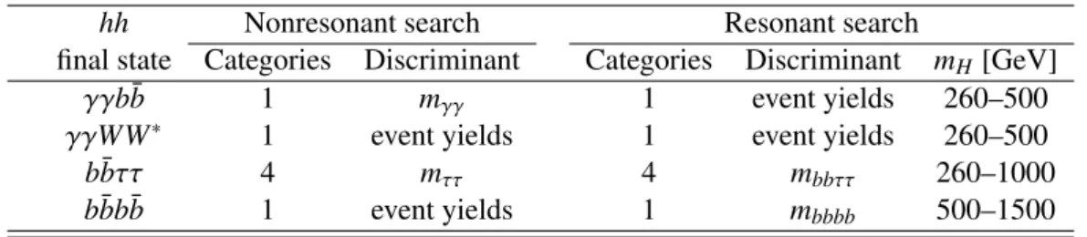
uncertainties used in the combinations are taken from Ref. [27]. Table3is a summary of the number of categories and final discriminants used for each analysis.
Table 3: An overview of the number of categories and final discriminant distributions used for both the nonresonant and resonant searches. Shown in the last column are the mass ranges of the resonant searches.
hh Nonresonant search Resonant search
final state Categories Discriminant Categories Discriminant mH[GeV]
γγb¯b 1 mγγ 1 event yields 260–500
γγWW∗ 1 event yields 1 event yields 260–500
b¯bττ 4 mττ 4 mbbττ 260–1000
b¯bb¯b 1 event yields 1 mbbbb 500–1500
The four individual analyses are sensitive to different kinematic regions of the hh production and decays. The combination is performed assuming that the relative contributions of these regions to the total cross section are modeled by the MadGraph5 [39] program used to simulate the hh production.
9 Results
In this section, the limits on the nonresonant and resonant searches are derived. The results of the hh → bbττ and hh→γγWW∗analyses are first determined and then combined with previously published results
of the hh → γγbb and hh → bbbb analyses. The impact of the leading systematic uncertainties is also discussed.
The observed and expected upper limits at 95% CL on the cross section of nonresonant production of a Higgs boson pair are shown in Table4. These limits are to be compared with the SM prediction of 9.9 ± 1.3 fb [17] for gg → hh production with mh= 125.4 GeV. Only the gluon fusion production process
is considered. The observed (expected) cross-section limits are 1.6 (1.3) pb and 11.4 (6.7) pb from the hh → bbττ and hh → γγWW∗analyses, respectively. Also shown in the table are the cross-section limits
relative to the SM expectation. The results are combined with those of the hh → γγbb and hh → bbbb analyses. The p-value of compatibility of the combination with the SM hypothesis is 4.4%, equivalent to 1.7 standard deviations. The low p-value is a result of the excess of events observed in the hh → γγbb analysis. The combined observed (expected) upper limit on σ(gg → hh) is 0.69 (0.47) pb, corresponding to 70 (48) times the cross section predicted by the SM. The hh → bbbb analysis has the best expected
sensitivity followed by the hh → γγbb analysis. The observed combined limit is slightly weaker than that of the hh → bbbb analysis, largely due to the aforementioned excess.
Table 4: The expected and observed 95% CL upper limits on the cross sections of nonresonant gg → hh production at √s= 8 TeV from individual analyses and their combinations. SM values are assumed for the h decay branching ratios. The cross-section limits normalized to the SM value are also included.
Analysis γγbb γγWW∗ bbττ bbbb Combined
Upper limit on the cross section [pb]
Expected 1.0 6.7 1.3 0.62 0.47
Observed 2.2 11 1.6 0.62 0.69
Upper limit on the cross section relative to the SM prediction
Expected 100 680 130 63 48
Observed 220 1150 160 63 70
The impact of systematic uncertainties on the cross-section limits is studied using the signal-strength parameter µ, defined as the ratio of the extracted to the assumed signal cross section (times branching ratio BR(H → hh) for the resonant search). The resulting shifts in µ depend on the actual signal-strength value. For illustration, they are evaluated using a cross section of 1 pb for gg → (H →)hh, comparable to the limits set. The effects of the most important uncertainty sources are shown in Table5. The leading contributions are from the background modeling, b-tagging, the h decay branching ratios, jet and EmissT measurements. The large impact of the b-tagging systematic uncertainty reflects the relatively large weight of the hh → bbbbanalysis in the combination. For the hh → bbττ analysis alone, the three leading systematic sources are the background estimates, jet and EmissT measurements, and lepton and τhad identifications. For the
hh →γγWW∗ analysis, they are the background estimates, jet and ETmiss measurements and theoretical uncertainties of the decay branching ratios of the Higgs boson h.
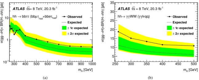
For the resonant production, limits are set on the cross section of gg → H production of the heavy Higgs boson times its branching ratio BR(H → hh) as a function of the heavy Higgs boson mass mH. The
observed (expected) limits of the hh → bbττ and hh → γγWW∗analyses are illustrated in Fig.5and listed
Table 5: The impact of the leading systematic uncertainties on the signal-strength parameter µ of a hypothesized signal for both the nonresonant and resonant (mH = 300, 600 GeV) searches. For the signal hypothesis, a Higgs
boson pair production cross section (σ(gg → hh) or σ(gg → H) × BR(H → hh)) of 1 pb is assumed.
Nonresonant search Resonant search
mH= 300 GeV mH = 600 GeV
Source ∆µ/µ [%] Source ∆µ/µ [%] Source ∆µ/µ [%]
Background model 11 Background model 15 b-tagging 10
b-tagging 7.9 Jet and Emiss
T 9.9 hBR 6.3
hBR 5.8 Lepton and τhad 6.9 Jet and EmissT 5.5
Jet and EmissT 5.5 hBR 5.9 Luminosity 2.7
Luminosity 3.0 Luminosity 4.0 Background model 2.4
in Table6(along with results from the hh → γγbb and hh → bbbb analyses). The mHsearch ranges are
260–1000 GeV for hh → bbττ and 260–500 GeV for hh → γγWW∗. For the hh → bbττ analysis, the observed limit around mH ∼ 300 GeV is considerably lower than the expectation, reflecting the deficit
in the observed mbbττ distribution. At high mass, the limits are correlated since a single bin is used
for mbbττ & 400 GeV. The decrease in the limit as mH increases is a direct consequence of increasing
selection efficiency for the signal. This is also true for the hh→γγWW∗analysis as the event selection is independent of mH. [GeV] H m 300 400 500 600 700 800 900 1000 hh) [pb] → BR(H × H) → (gg σ -1 10 1 10 Observed Expected expected σ 1 ± expected σ 2 ± ATLAS s= 8 TeV, 20.3 fb-1 ) had τ +bbe had τ µ (bb τ τ bb → hh (a) [GeV] H m 250 300 350 400 450 500 hh) [pb] → BR(H × H) → (gg σ 5 10 15 20 25 30 35 Observed Expected expected σ 1 ± expected σ 2 ± ATLAS s = 8 TeV,20.3 fb-1 qq) ν l γ γ WW ( γ γ → hh (b)
Figure 5: The observed and expected upper limit at 95% CL on σ(gg → H) × BR(H → hh) at √s = 8 TeV as a function of mHfrom the resonant (a) hh → bbττ and (b) hh → γγWW∗analyses. The search ranges of the resonance
mass are 260–1000 GeV for hh → bbττ and 260–500 GeV for hh → γγWW∗. The green and yellow bands represent ±1σ and ±2σ ranges on the expected limits, respectively.
Table 6: The expected and observed 95% CL upper limits on σ(gg → H) × BR(H → hh) in pb at √s= 8 TeV from individual analyses and their combinations. The SM branching ratios are assumed for the light Higgs boson decay.
mH Expected limit [pb] Observed limit [pb]
[GeV] γγbb γγWW∗ bbττ bbbb Combined γγbb γγWW∗ bbττ bbbb Combined
260 1.70 11.2 2.6 – 1.1 2.29 18.7 4.2 – 2.1 300 1.53 9.3 3.1 – 1.2 3.54 15.1 1.7 – 2.0 350 1.23 7.8 2.2 – 0.89 1.44 13.3 2.8 – 1.5 400 1.00 6.9 0.97 – 0.56 1.00 11.5 1.5 – 0.83 500 0.72 5.9 0.66 – 0.38 0.71 10.9 1.0 – 0.61 500 – – 0.66 0.17 0.16 – – 1.0 0.16 0.18 600 – – 0.48 0.070 0.067 – – 0.79 0.072 0.079 700 – – 0.31 0.041 0.040 – – 0.61 0.038 0.040 800 – – 0.31 0.028 0.028 – – 0.51 0.046 0.049 900 – – 0.30 0.022 0.022 – – 0.48 0.015 0.015 1000 – – 0.28 0.018 0.018 – – 0.46 0.011 0.011
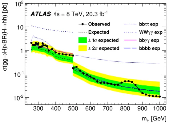
The hh → γγbb and hh → bbbb analyses are published separately and the mass range covered by the two analyses are 260–500 GeV and 500–1500 GeV, respectively. The results of these four analyses, summarized in Table6, are combined for the mass range 260–1000 GeV assuming the SM values of the
hdecay branching ratios. To reflect the better mass resolutions of the hh → bbbb and hh → γγbb analyses, the combination is performed with smaller mass steps than those of the hh → bbττ and hh → γγWW∗ analyses. The most significant excess in the combined results is at a resonance mass of 300 GeV with a local significance of 2.5σ, largely due to the 3.0σ excess observed in the hh → γγbb analysis [21]. The upper limit on σ(gg → H) × BR(H → hh) varies from 2.1 pb at 260 GeV to 0.011 pb at 1000 GeV. These limits are shown in Fig.6 as a function of mH. For the low-mass region of 260–500 GeV, both
the hh → γγbb and hh → bbττ analyses contribute significantly to the combined sensitivities. Above 500 GeV, the sensitivity is dominated by the hh → bbbb analysis. Table5shows the impact of the leading systematic uncertainties for a heavy Higgs boson mass of 300 GeV and 600 GeV. As in the nonresonant search, the systematic uncertainties with the largest impact on the sensitivity are from the uncertainties on the background modeling, b-tagging, jet and ETmiss measurements, and the h decay branching ratios. These limits are directly applicable to models such as those of Refs. [72–77] in which the Higgs boson h has the same branching ratios as the SM Higgs boson.
[GeV]
Hm
300
400
500
600
700
800
900 1000
hh) [pb]
→
BR(H
×
H)
→
(gg
σ
-210
-110
1
10
210
exp τ τ bb exp γ γ WW exp γ γ bb bbbb exp Observed Expected expected σ 1 ± expected σ 2 ±ATLAS
ATLAS
s
= 8 TeV, 20.3 fb
-1Figure 6: The observed and expected 95% CL upper limits on σ(gg → H) × BR(H → hh) at √s = 8 TeV as functions of the heavy Higgs boson mass mH, combining resonant searches in hh → γγbb, bbbb, bbττ and γγWW∗
final states. The expected limits from individual analyses are also shown. The combination assumes SM values for the decay branching ratios of the lighter Higgs boson h. The green and yellow bands represent ±1σ and ±2σ uncertainty ranges of the expected combined limits. The improvement above mH= 500 GeV is due to the sensitivity
of the hh → bbbb analysis. The more finely spaced mass points of the combination reflect the better mass resolutions of the hh → γγbb and hh → bbbb analyses than those of the hh → bbττ and hh → γγWW∗analyses.
10 Interpretation
The upper cross-section limits of the resonant search are interpreted in two MSSM scenarios, one referred to as the hMSSM [28,29] and the other as the low-tb-high [30]. In the interpretation, the CP-even light and heavy Higgs bosons of the MSSM are assumed to be the Higgs bosons h and H of the search, respectively. The natural width of the heavy Higgs boson H where limits are set in these scenarios is sufficiently smaller than the experimental resolution, which is at best 1.5%, that its effect can be neglected.
In the hMSSM scenario, the mass of the light CP-even Higgs boson is fixed to 125 GeV in the whole parameter space. This is achieved by implicitly allowing the supersymmetry-breaking scale mSto be very
large, which is especially true in the low tan β region where mS 1 TeV, and making assumptions about
the CP-even Higgs boson mass matrix and its radiative corrections, as well as the Higgs boson coupling dependence on the MSSM parameters. Here tan β is the ratio of the vacuum expectation values of the two doublet Higgs fields. The “low-tb-high” MSSM scenario follows a similar approach, differing in that explicit choices are made for the supersymmetry-breaking parameters [30]. The mass of the light Higgs boson is not fixed in this scenario, but is approximately 125 GeV in most of the parameter space. The mh
value grows gradually from 122 GeV at mA ∼ 220 GeV to 125 GeV as mA approaching infinity. Higgs
boson production cross sections through the gluon-fusion process are calculated with SusHi 1.4.1 [78–80] for both scenarios. Higgs boson decay branching ratios are calculated with HDECAY 6.42 [81] following the prescription of Ref. [29] for the hMSSM scenario and with FeynHiggs 2.10.0 [82–84] for the low-tb-high scenario.
The upper limits on σ(gg → H) × BR(H → hh) can be interpreted as exclusion regions in the (tan β, mA)
plane. In both scenarios, the Higgs boson pair production rate σ(gg → H) × BR(H → hh) depends on tan β and the mass of the CP-odd Higgs boson (mA), and so does the mass of the heavy CP-even Higgs
boson H. The values of mA and mH are generally different: mH can be as much as 70 GeV above mA in
the parameter space relevant for this publication with the difference in masses decreasing for increasing values of tan β or mA. Constant mH lines for a few selected values are shown in Fig. 7. The decay
branching ratios of the light Higgs boson in these scenarios depend on tan β and mA and are different
from the corresponding SM values used to derive the upper limits shown in Table6. The upper limits, as functions of mH, are recomputed; the hh decay fractions for each final state are fixed to their smallest
value found in 1 < tan β < 2, the range of the expected sensitivity. This approach yields conservative limits, but simplifies the computation as the limit calculation does not have to be repeated at each tan β value. The results are used to set exclusions in the (tan β, mA) plane as shown in Fig. 7. The analysis
is sensitive to the region of low tan β and mA values in the range ∼ 200–350 GeV. For mA . 200 GeV,
mH is typically below the 2mh threshold of the H → hh decay, whereas above 350 GeV, the H → hh
decay is suppressed because of the dominance of the H → t¯t decay. The observed exclusion region in the (tan β, mA) plane is smaller than the expectation, reflecting the small excess observed in the data.
11 Summary
This paper summarizes the search for both nonresonant and resonant Higgs boson pair production in proton–proton collisions from approximately 20 fb−1of data at a center-of-mass energy of 8 TeV recorded by the ATLAS detector at the LHC. The search is performed in hh → bbττ and γγWW∗final states. No significant excess is observed in the data beyond the background expectation. Upper limits on the hh production cross section are derived. Combining with the hh → γγbb, bbbb searches, a 95% CL upper
[GeV] A m 220 240 260 280 300 320 340 360 380 400 β tan 1 1.2 1.4 1.6 1.8 2 2.2 2.4 250 275 300 325 350 375 hMSSM -1 = 8 TeV, 20.3 fb s ATLAS
Observed exclusion Expected exclusion (GeV) H Constant m ± 1 σ expected (a) [GeV] A m 220 240 260 280 300 320 340 360 380 400 β tan 1 1.2 1.4 1.6 1.8 2 2.2 2.4 250 275 300 325 350 375 low-tb-high -1 = 8 TeV, 20.3 fb s ATLAS
Observed exclusion Expected exclusion (GeV) H Constant m ± 1 σ expected < 122 GeV h m (b)
Figure 7: The observed and expected 95% CL exclusion regions in the (tan β, mA) plane of MSSM scenarios from
the resonant search: (a) the hMSSM scenario and (b) the low-tb-high scenario. The green dotted lines delimit the ±1σ uncertainty ranges of the expected exclusion regions. The gray dashed lines show the constant values of the heavy CP-even Higgs boson mass. The improved sensitivity in the expected exclusion on the contour line of mH ∼ 260 GeV reflects the improved expected limit on the cross section while the hole or the wedge around the
mH ∼ 325 GeV contour line in the observed exclusion is the result of a small excess at this mass, see Fig.6. The
gray shaded region in (b) shows the region where the mass of the light CP-even Higgs boson is inconsistent with the measured value of 125.4 GeV. There is no such region in (a) by construction.
limit of 0.69 pb on the cross section of the nonresonant hh production is observed compared with the expected limit of 0.47 pb. This observed upper limit is approximately 70 times the SM gg → hh production cross section. For the production of a narrow heavy resonance decaying to a pair of light Higgs bosons, the observed (expected) upper limit on σ(gg → H) × BR(H → hh) varies from 2.1 (1.1) pb at 260 GeV to 0.011 (0.018) pb at 1000 GeV. These limits are obtained assuming SM values for the h decay branching ratios. Exclusion regions in the parameter space of simplified MSSM scenarios are also derived.
Acknowledgments
We thank CERN for the very successful operation of the LHC, as well as the support staff from our institutions without whom ATLAS could not be operated efficiently.
We acknowledge the support of ANPCyT, Argentina; YerPhI, Armenia; ARC, Australia; BMWFW and FWF, Austria; ANAS, Azerbaijan; SSTC, Belarus; CNPq and FAPESP, Brazil; NSERC, NRC and CFI, Canada; CERN; CONICYT, Chile; CAS, MOST and NSFC, China; COLCIENCIAS, Colombia; MSMT CR, MPO CR and VSC CR, Czech Republic; DNRF, DNSRC and Lundbeck Foundation, Den-mark; IN2P3-CNRS, CEA-DSM/IRFU, France; GNSF, Georgia; BMBF, HGF, and MPG, Germany; GSRT, Greece; RGC, Hong Kong SAR, China; ISF, I-CORE and Benoziyo Center, Israel; INFN, Italy; MEXT and JSPS, Japan; CNRST, Morocco; FOM and NWO, Netherlands; RCN, Norway; MNiSW and NCN, Poland; FCT, Portugal; MNE/IFA, Romania; MES of Russia and NRC KI, Russian Feder-ation; JINR; MESTD, Serbia; MSSR, Slovakia; ARRS and MIZŠ, Slovenia; DST/NRF, South Africa; MINECO, Spain; SRC and Wallenberg Foundation, Sweden; SERI, SNSF and Cantons of Bern and
Geneva, Switzerland; MOST, Taiwan; TAEK, Turkey; STFC, United Kingdom; DOE and NSF, United States of America. In addition, individual groups and members have received support from BCKDF, the Canada Council, CANARIE, CRC, Compute Canada, FQRNT, and the Ontario Innovation Trust, Canada; EPLANET, ERC, FP7, Horizon 2020 and Marie Skłodowska-Curie Actions, European Union; Investisse-ments d’Avenir Labex and Idex, ANR, Region Auvergne and Fondation Partager le Savoir, France; DFG and AvH Foundation, Germany; Herakleitos, Thales and Aristeia programmes co-financed by EU-ESF and the Greek NSRF; BSF, GIF and Minerva, Israel; BRF, Norway; the Royal Society and Leverhulme Trust, United Kingdom.
The crucial computing support from all WLCG partners is acknowledged gratefully, in particular from CERN and the ATLAS Tier-1 facilities at TRIUMF (Canada), NDGF (Denmark, Norway, Sweden), CC-IN2P3 (France), KIT/GridKA (Germany), INFN-CNAF (Italy), NL-T1 (Netherlands), PIC (Spain), ASGC (Taiwan), RAL (UK) and BNL (USA) and in the Tier-2 facilities worldwide.
References
[1] ATLAS Collaboration, Observation of a new particle in the search for the Standard Model Higgs boson with the ATLAS detector at the LHC, Phys. Lett. B716 (2012) 1,
arXiv:1207.7214 [hep-ex]. [2] CMS Collaboration,
Observation of a new boson at a mass of 125 GeV with the CMS experiment at the LHC, Phys. Lett. B716 (2012) 30–61, arXiv:1207.7235 [hep-ex].
[3] ATLAS Collaboration, Measurements of Higgs boson production and couplings in diboson final states with the ATLAS detector at the LHC, Phys. Lett. B726 (2013) 88,
arXiv:1307.1427 [hep-ex]. [4] CMS Collaboration,
Precise determination of the mass of the Higgs boson and tests of compatibility of its couplings with the standard model predictions using proton collisions at 7 and 8 TeV,
Eur. Phys. J. C75 (2015) 212, arXiv:1412.8662 [hep-ex].
[5] ATLAS Collaboration, Search for the b¯b decay of the Standard Model Higgs boson in associated (W/Z)H production with the ATLAS detector, JHEP 1501 (2015) 069,
arXiv:1409.6212 [hep-ex]. [6] ATLAS Collaboration,
Evidence for the Higgs-boson Yukawa coupling to tau leptons with the ATLAS detector, JHEP 1504 (2015) 117, arXiv:1501.04943 [hep-ex].
[7] ATLAS Collaboration, Evidence for the spin-0 nature of the Higgs boson using ATLAS data, Phys. Lett. B726 (2013) 120, arXiv:1307.1432 [hep-ex].
[8] CMS Collaboration, Constraints on the spin-parity and anomalous HVV couplings of the Higgs boson in proton collisions at 7 and 8 TeV, Phys. Rev. D92 (2015) 012004,
arXiv:1411.3441 [hep-ex].
[9] U. Baur, T. Plehn and D. L. Rainwater,
Determining the Higgs Boson Self Coupling at Hadron Colliders, Phys. Rev. D67 (2003) 033003, arXiv:hep-ph/0211224 [hep-ph].