HAL Id: hal-00676807
https://hal.archives-ouvertes.fr/hal-00676807
Submitted on 6 Jun 2015
HAL is a multi-disciplinary open access
archive for the deposit and dissemination of
sci-entific research documents, whether they are
pub-lished or not. The documents may come from
teaching and research institutions in France or
abroad, or from public or private research centers.
L’archive ouverte pluridisciplinaire HAL, est
destinée au dépôt et à la diffusion de documents
scientifiques de niveau recherche, publiés ou non,
émanant des établissements d’enseignement et de
recherche français ou étrangers, des laboratoires
publics ou privés.
2010/2011: comparison with 1996/1997
Jayanarayanan Kuttippurath, Sophie Godin-Beekmann, Franck Lefèvre, G.
Nikulin, M. L. Santee, L. Froidevaux
To cite this version:
Jayanarayanan Kuttippurath, Sophie Godin-Beekmann, Franck Lefèvre, G. Nikulin, M. L. Santee,
et al.. Record-breaking ozone loss in the Arctic winter 2010/2011: comparison with 1996/1997.
Atmospheric Chemistry and Physics, European Geosciences Union, 2012, 12 (15), pp.7073-7085.
�10.5194/acp-12-7073-2012�. �hal-00676807�
Atmos. Chem. Phys., 12, 7073–7085, 2012 www.atmos-chem-phys.net/12/7073/2012/ doi:10.5194/acp-12-7073-2012
© Author(s) 2012. CC Attribution 3.0 License.
Atmospheric
Chemistry
and Physics
Record-breaking ozone loss in the Arctic winter 2010/2011:
comparison with 1996/1997
J. Kuttippurath1, S. Godin-Beekmann1, F. Lef`evre1, G. Nikulin2, M. L. Santee3, and L. Froidevaux3
1UPMC Universit´e Paris 06, LATMOS-IPSL, CNRS/INSU, UMR8190, 75005 Paris, France 2Swedish Meteorological Hydrological Institute, Kiruna, Sweden
3JPL/NASA, California Institute of Technology, Pasadena, California, USA
Correspondence to: J. Kuttippurath ([email protected])
Received: 5 February 2012 – Published in Atmos. Chem. Phys. Discuss.: 6 March 2012 Revised: 25 July 2012 – Accepted: 27 July 2012 – Published: 6 August 2012
Abstract. We present a detailed discussion of the chemical
and dynamical processes in the Arctic winters 1996/1997 and 2010/2011 with high resolution chemical transport model (CTM) simulations and space-based observations. In the Arctic winter 2010/2011, the lower stratospheric minimum temperatures were below 195 K for a record period of time, from December to mid-April, and a strong and stable vor-tex was present during that period. Simulations with the Mimosa-Chim CTM show that the chemical ozone loss started in early January and progressed slowly to 1 ppmv (parts per million by volume) by late February. The loss intensified by early March and reached a record maximum of ∼2.4 ppmv in the late March–early April period over a broad altitude range of 450–550 K. This coincides with el-evated ozone loss rates of 2–4 ppbv sh−1 (parts per billion
by volume/sunlit hour) and a contribution of about 30–55 % and 30–35 % from the ClO-ClO and ClO-BrO cycles, re-spectively, in late February and March. In addition, a con-tribution of 30–50 % from the HOx cycle is also estimated
in April. We also estimate a loss of about 0.7–1.2 ppmv con-tributed (75 %) by the NOxcycle at 550–700 K. The ozone
loss estimated in the partial column range of 350–550 K ex-hibits a record value of ∼148 DU (Dobson Unit). This is the largest ozone loss ever estimated in the Arctic and is consis-tent with the remarkable chlorine activation and strong den-itrification (40–50 %) during the winter, as the modeled ClO shows ∼1.8 ppbv in early January and ∼1 ppbv in March at 450–550 K. These model results are in excellent agreement with those found from the Aura Microwave Limb Sounder observations. Our analyses also show that the ozone loss in 2010/2011 is close to that found in some Antarctic winters,
for the first time in the observed history. Though the win-ter 1996/1997 was also very cold in March–April, the tem-peratures were higher in December–February, and, therefore, chlorine activation was moderate and ozone loss was average with about 1.2 ppmv at 475–550 K or 42 DU at 350–550 K, as diagnosed from the model simulations and measurements.
1 Introduction
Chemical ozone loss in the Arctic stratosphere has been ob-served since 1989. Since then, cold winters are prone to large chemical ozone loss due to the still high amounts of ozone depleting substances in the atmosphere (Rex et al., 2004). However, because of large planetary wave activity, the polar vortex breaks up or dissipates early in most Arc-tic winters (WMO, 2011; Harris et al., 2010; Kuttippurath et al., 2010b; Manney et al., 2003). Therefore, the vortex per-sistence has been comparatively shorter and the associated ozone loss smaller in the Arctic as compared to the Antarctic (WMO, 2011; Solomon et al., 2007). The longest vortex per-sistence in the Arctic was found in 1996/1997, in which the wave activity was considerably suppressed, and therefore the vortex was sustained until early May (Lef`evre et al., 1998; Coy et al., 1997). Nevertheless, the ozone loss in 1996/1997 was lower than that of other cold winters such as 1994/1995, 1999/2000, and 2004/2005 due to relatively higher tempera-tures in December–February 1996/1997, when chlorine acti-vation plays a key role in determining the magnitude of ozone loss (Manney et al., 2003; Santee et al., 1997). In contrast, very low temperatures were observed in March–April due
to a high tropopause associated with a tropospheric block-ing durblock-ing the 1996/1997 Arctic winter (Coy et al., 1997). A similar evolution in temperature and vortex persistence was also observed in spring 2011 (Hurwitz et al., 2011; Manney et al., 2011), during which the stratospheric halogen loading was very similar to that in 1996/1997. Note that long per-sistence of a cold vortex is a necessary requirement for the sustained ozone loss. Studies have already shown prolonged appearance of very low temperatures and exceptional ozone loss in 2010/2011 (Balis et al., 2011; Manney et al., 2011; Sinnhuber et al., 2011). Persistence of very low tempera-tures and strong vortices for a record period of time, and very late final warmings were the common features of the Arctic winters 1996/1997 and 2010/2011. The vortex in 1996/1997 was even stronger and the final warming was later than in 2010/2011. However, the chemical processing and ozone loss were different in these winters. Therefore, the situations in both winters merit a close examination to diagnose the sim-ilarities and differences between the polar processing of the winters and to find possible reasons for them. The winters are analyzed with high resolution chemical transport model simulations and satellite measurements to further elucidate the ozone loss processes.
This article is arranged in the following order: Sect. 2 describes the data and methods, including the model sim-ulations, the MLS measurements and European Centre for Medium-Range Weather Forecasts (ECMWF) data. The re-sults from the study are discussed in Sect. 3, in which me-teorology (Sect. 3.1) and ozone loss (Sect. 3.2) during the winters 1996/1997 and 2010/2011 are presented. A detailed characterization of the dynamics of both winters is presented in this part with temperature and zonal wind, and heat flux and wave amplitude calculations. In addition, the time evo-lution of the polar vortex is demonstrated with potential vor-ticity (PV) maps. Apart from the ozone loss calculations by the passive method, the ozone loss and production rates, and the contribution of various chemical cycles to the ozone loss are given in Sect. 3.3 to help the interpretation of the derived ozone loss. The vertical features of ozone loss are compared to the partial column ozone loss estimations from both sim-ulations and measurements and are discussed in Sect. 3.4. Sect. 3.5 compares the ozone loss estimated in this study with other available ones. The atypical ozone loss that occurred in the Arctic winter 2010/2011 is compared to the Antarctic ozone loss in Sect. 4. The primary findings of this study are summarized in Sect. 5.
2 Data and method
We use the high resolution chemical transport model (CTM) Mimosa-Chim for this study (e.g. Kuttippurath et al., 2010b; Tripathi et al., 2006). The model has 1 × 1◦horizontal res-olution in the spatial domain of 10◦S–90◦N with 25 isen-tropical vertical levels between 350 K and 950 K, with 5 K
resolution between 425 K and 550 K to study the ozone de-pletion layers closely. The ECMWF analyses are used to force the model runs, and the model uses the MIDRAD ra-diation scheme (Shine, 1987). The chemical fields of the model runs are initialized from the 3-D CTM REPROBUS output (Lef`evre et al., 1998). The kinetic data are taken from Sander et al. (2006), but the Cl2O2cross-sections are from
Burkholder et al. (1990), with a log-linear extrapolation up to 450 nm as suggested by Stimpfle et al. (2004). Although there are new measurements for Cl2O2(Papanastasiou et al.,
2009), the differences in the simulated ozone loss among various sensitivity runs are very small (2 %) (Kuttippurath et al., 2010b). The model has detailed polar stratospheric cloud (PSC) and sedimentation schemes. As we use the same model and run procedures, further details of the model runs can be found in Kuttippurath et al. (2010b). For the winters considered here, the model was run from 1 December to 30 April. We use the passive tracer method (WMO, 2007 and references therein) to derive ozone depletion, for which the ozone (O3) and passive tracer are initialized together in the
beginning of each simulation, and then the ozone loss is es-timated as Mimosa-Chim O3or MLS O3minus the passive
tracer.
To compare with the simulations, we use measurements of O3and chlorine monoxide (ClO) from the Upper
Atmo-sphere Research Satellite (UARS) Microwave Limb Sounder (MLS) version (v)5 for the winter 1996/1997 and the Aura MLS v3.3 for the winter 2010/2011. The UARS MLS O3
profiles have a vertical range of about 15–60 km and a ver-tical resolution of ∼3–4 km. The uncertainty of a typical O3measurement is 6–15 % over 16–60 km. The Aura MLS
O3measurements have a vertical range of about 12–73 km
with a vertical resolution of 2.5–3 km and an uncertainty of 5–10 % between 68 hPa and 0.2 hPa. The vertical range of UARS MLS ClO profiles is 100–1 hPa, with a vertical resolution of 4–5 km and an uncertainty of 20 % at 46 hPa, whereas the Aura MLS ClO has a vertical resolution of 3– 3.5 km and a vertical range of 100–0.1 hPa. The uncertainty of Aura MLS ClO retrievals is about 10–20 %, depending on altitude. In order to screen the UARS MLS data we have used the guidelines provided by Livesey et al. (2003), with only profiles with positive precision values, Quality values (= 4), and “MMAF STAT” flags with “G”, “t”, or “T” be-ing considered. We have also subtracted altitude dependent known biases identified in the UARS ClO profiles prior to their interpolation to specific potential temperature levels. The selection of Aura MLS profiles are based on their Con-vergence, Quality, Status, and Precision values as recom-mend by Livesey et al. (2011) for each molecule. In addi-tion, latitude-dependent biases at 146, 100 and 68 hPa are subtracted from the ClO profiles before their vertical inter-polation. Further details about the data and data screening procedures can be found in Livesey et al. (2003) for UARS MLS and Froidevaux et al. (2008), Santee et al. (2008), and Livesey et al. (2011) for Aura MLS.
J. Kuttippurath et al.: Exceptional Arctic ozone loss in 2011 7075
12 J. Kuttippurath et al.: Exceptional Arctic ozone loss in 2011
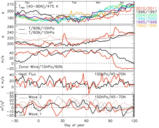
Fig. 1. Temporal evolution of minimum temperature at 475 K (top plot), temperature at 60◦N and 90◦N at 10 hPa (second plot from the top),
zonal wind at 60◦N/10 hPa (third plot from the top), heat flux (fourth plot from the top), and planetary wave amplitudes (bottom) for the
Arctic winters 1996/1997 (black) and 2010/2011 (red). The heat flux and wave amplitudes are averaged between 45◦N and 70◦N at 100 hPa.
The minimum temperatures during the cold Arctic winters 1994/1995 (yellow), 1995/1996 (violet), 1999/2000 (blue) and 2004/2005 (green) are also shown. The dash-dotted line represents 195 K temperature, the dashed lines mark the zero-wind line, zero heat flux or zero wave amplitude in the respective plots, and dotted vertical lines differentiate the approximate boundaries of each month.
We use the ECMWF operational meteorological analyses to calculate the minimum temperature, PV, heat flux, plane-tary waves, and vortex edge. The ECMWF data archived at the Norwegian Institute for Air Research (NILU) data base are used in this study. These analyses have a horizontal reso-lution of 2.5×2.5◦and are available at 1000, 700, 500, 300, 200, 150, 100, 70, 50, 30 and 10 hPa pressure levels (e.g. Woods, 2006).
3 Results and discussion
3.1 Synoptic evolution of the winters
Figure 1 shows the minimum temperature extracted north of 40◦N, zonal wind, heat flux and the wave 1 and 2 calculated from geopotential fields for the Arctic winters 1996/1997 and 2010/2011. In 1996/1997, the minimum temperatures show values above and below 195 K in December and January– March, respectively. On the other hand, temperatures below 195 K from December through early April are observed in 2010/2011 (Manney et al., 2011). So the minimum
temper-ature in 2010/2011 is consistently lower than in 1996/1997 throughout the winter by about 2–10 K. As compared to other cold winters in the Arctic, the temperature in 2010/2011 is similar until mid-February, but about 10–20 K lower than that of other winters in March–April, indicating the longest period of low temperatures in the last two decades (Man-ney et al., 2011; Sinnhuber et al., 2011). The temperature in 1996/1997 is also lower than that in 1994/1995, 1999/2000 and 2004/2005 from mid-March to April, but is about 10– 20 K higher in December–February than all other winters. It should be recalled that these analyses hold for 475 K only. The winters 1999/2000, 2004/2005, and 2010/2011 exhibit the lowest minimum temperature of about 182 K around 20 January.
To diagnose sudden stratospheric warmings, the temper-ature at 60◦N/10 hPa and 90◦N/10 hPa and zonal winds
at 60◦N/10 hPa are analyzed. In 1996/1997, there were no warmings and the westerlies were strong with a speed of
∼40 m s−1in January–April, with the final warming unusu-ally late in early May. In contrast, two minor warmings with a magnitude of about 10 K and 40 K at 90◦N/10 hPa in early
200 205 205 205 205 205 210 210 215 215 220 220 225 Dec. 05 1996/1997 195 200 205 205 205 205 210 210 210 210 215 215 215 215 220 220 220 225 Jan. 28 195 200 205 205 205 205 210 210 210 215 215 215 220 220 220 Feb. 03 195 200 205 205 205 205 210 210 210 215 215 215 215 220 220 220 Mar. 14 pvu 475 K 205 205 205205 210 210 210 215 215 215 220 220 225 Apr. 21 200 205 205 205 205 205 205 210 210 210 210 215 215 220 220 2010/2011 190 195200 205 205 205 205 205 205 205 210 210 210 215 215 215 220 220 220 225 200 200 205 205 205 205 210 210 210 215 215 220 220 225 225 195 200 205 205 205 205 210 210 210 215 215 215 215 215 220 205 205 205 205 210 210 210 215 215 220 220 225230
10
20
30
40
50
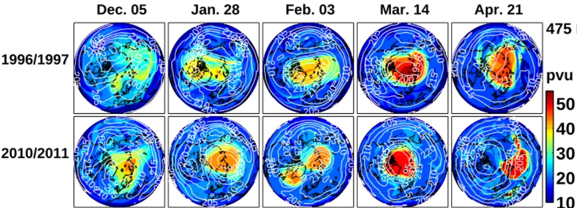
Fig. 2. Temporal evolution of the polar vortex during selected days of the Arctic winters 1996/1997 (upper panel) and 2010/2011 (lower
panel) at 475 K potential temperature level. The days are selected by analyzing the complete record of the winter to fairly represent the temporal evolution. The overlaid white contours are temperature in Kelvin. The blue/red colors show relatively low/high potential vorticity
units (pvu), where 1 pvu is 10−6km2kg−1s−1.
January and early February, respectively, were observed in 2010/2011. These warmings lasted for a week, and were due to wave 1 and wave 2 amplifications, with zonal mean heat fluxes (v0T0at 45–70◦N/100 hPa) of about 34 K m s−1. Nev-ertheless, strong westerlies with a speed of ∼40 m s−1were present from December to the end of March in 2010/2011. The temperatures began to increase by the second week of April and the winds turned to easterly, indicating the fi-nal warming, which was about two weeks earlier than in 1996/1997. The heat flux, Eliassen-Palm (EP) divergence, and EP flux of the waves 1 and 2 (not shown) show very small or near zero values in February–early April in both winters. This implies that there was no significant wave activity to warm the stratosphere up, and hence, the temperature stayed cold and winds remained westerly to sustain a stable vor-tex during the period. However, the heat flux in February– April and wave amplitudes in March–April show compara-tively smaller amplitude in 1996/1997, indicating very weak wave driving during the winter. Therefore, prolonged persis-tence of lower temperatures, larger zonal wind amplitudes, and hence, an exceptionally late final warming are observed in the Arctic winter 1996/1997. Further details about the dy-namical processes of both winters can be found in Hurwitz et al. (2011).
Figure 2 shows PV maps at 475 K on selected days of both winters. In 1996/1997 (top panel), the vortex was rela-tively large, stable and pole-centered for most days until late April. In December the vortex was undisturbed, but a minor warming occurred in early January. The vortex was unusually strong in February through mid-April, during which the vor-tex was mostly pole-centered and large in size. In contrast, in 2010/2011 (bottom panel), the vortex formed in early De-cember with considerable size. Though the minor warming moved the vortex slightly off the pole in January, the vortex was still strong with PV values of ∼50 pvu (PV units; 1 pvu is 10−6Km2kg−1s−1). The vortex stayed pole-centered again
until the minor warming in early February, during which the vortex nearly split into two parts. Since the warming was short and the westerlies were strong, the vortex merged and regained its strength to form a large pole-centered one after a few days and stayed intact until late April 2011. Note that the vortex was still significantly smaller than that of other cold Arctic winters in February–April, including the winter 1996/1997 as shown by the PV maps in Fig. 2 and mentioned by Manney et al. (2011). In April, the temperatures began to increase and westerlies started to diminish, and the vor-tex tilted off the pole and, then stayed mostly in the midlati-tudes until the final warming in late April. The vortex evolu-tion was similar at most altitudes between 450 K and 850 K, but the vortex dissipation was observed a few days earlier at 850 K in both winters.
3.2 PSCs, chlorine activation and ozone loss 3.2.1 Winter 1996/1997
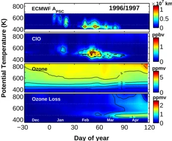
Figure 3 shows the potential PSC areas, and the vortex-averaged Mimosa-Chim simulations of ClO, O3, and ozone
loss for the Arctic winter 1996/1997. The ClO data are fil-tered with respect to a criterion of 12:00 UT and solar zenith angle less than 89◦. In this study the area of PSCs (APSC)
is considered as the area where temperatures are less than the Nitric Acid Tri-hydrate (NAT) threshold, TNAT. The TNAT
estimation is done by applying the scheme of Hanson and Mauersberger (1988) using the ECMWF temperature and pressure analyses, with 4.5 ppmv (parts per million by vol-ume) of H2O and a HNO3 climatology (Rex et al., 2004;
Kuttippurath et al., 2010b).
As the temperatures are above 195 K, no PSCs are found in December. In January, PSCs with areas of ∼0.7 × 10⁷km2 are estimated at 500–600 K. Large areas of PSCs with a max-imum of about 1.3 × 10⁷km2 are found at 400–550 K until mid-March and there were no PSCs afterwards, consistent
J. Kuttippurath et al.: Exceptional Arctic ozone loss in 2011 7077 0.4 0.4 ECMWF APSC 1996/1997 × 107 km2 400 600 800 0 0.5 1 0.4 0.8 ClO Potential Temperature (K) ppbv 400 600 800 0 1 1 2 3 4 5 Ozone ppmv 400 600 800 0 5 0.5 1 Ozone Loss ppmv Day of year
Dec Jan Feb Mar Apr
−30 0 30 60 90 120 400 600 800 0 1 2
Fig. 3. Temporal evolution of the vertical distribution of potential
PSC areas (top) and Mimosa-Chim simulations of ClO (second plot
from the top), O3(third plot from the top), and ozone loss (bottom)
inside the vortex for the Arctic winter 1996/1997. The ClO profiles
are selected at 12 UT and solar zenith angles below 89◦. The white
dotted lines represent 475 K and 675 K. The blue/red colors show relatively low/high values of PSC areas or mixing ratios of ClO,
O3, and ozone loss.
with the temperatures during the period. So the chlorine ac-tivation was moderate, as indicated by the ClO mixing ratios of ∼0.7 ppbv (parts per billion by volume) in mid-January, about 1–1.7 ppbv in mid-February and about 0.5 ppbv in March around 475 K. Since the vortex was symmetric and pole-centered, there were no changes in O3 distributions
at most altitudes until late February, but a reduction of 1– 1.3 ppmv was found thereafter in the lower stratosphere in the sunlit parts of the vortex. This change in O3is evident
when following the 3 ppmv and 4 ppmv O3 isopleths. The
corresponding ozone loss is about 0.6 ppmv in late Febru-ary and 1.2 ppmv in late March–April around 475 K. There is also a significant loss of 0.4–0.7 ppmv, by NOx catalytic
chemistry, at altitudes above 550 K up to 700 K in April. Since the denitrification in the winter 1996/1997 was studied extensively (e.g. Kondo et al., 2000; Santee et al., 1999) and was not severe as in other cold Arctic winters (e.g. Kleinb¨ohl et al., 2005), we have excluded discussions on denitrification in this winter.
Figure 4 compares the ClO, O3, and ozone loss
simula-tions with those from the UARS MLS measurements. Here data are selected with respect to the MLS sampling points inside the vortex and hence, these are slightly different from the vortex averages shown in Fig. 3. The model results are in reasonable agreement with the observations. The simulated ClO is slightly lower (e.g. Santee et al., 1997) and O3is a
little higher, and thus, the simulated ozone loss is about 0.1– 0.2 ppmv lower than in the observations at 425–550 K. Still
the measurements also show a peak loss of about 1.2 ppmv by late April. In addition, our results are in good agree-ment with those of Manney et al. (2003, 1997) and Knud-sen et al. (1998), who estimate a peak ozone loss of about 1.2 ppmv at 465 K and 1.24 ppmv at 475 K by late March from UARS MLS and ozonesonde measurements, respec-tively. The SLIMCAT model also calculates a similar ozone loss maximum of about 1.1 ppmv at 475 K in late March (Hanson and Chipperfield, 1999).
3.2.2 Winter 2010/2011
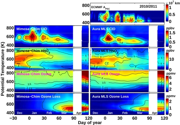
Figure 5 presents the modeled and measured ClO, HNO3,
O3, and ozone loss at the Aura MLS sampling locations
in-side the vortex, together with the area of PSCs, for the win-ter 2010/2011. Large areas of PSCs with maximum values of about 1.1 × 10⁷km2are estimated from mid-December to late March. Note that the APSC in 2010/2011 is
systemati-cally larger than that in 1996/1997 both with time and alti-tude. This suggests that the winter 2010/2011 had an unusu-ally long period of PSC appearance in a wide vertical extent between 400 K and 600 K compared to any other Arctic win-ter (Manney et al., 2011; Kuttippurath et al., 2010b).
Consistent with the APSC, about 0.5–0.7 ppbv of ClO in
December and 1–1.8 ppbv of ClO in January–March at 450– 600 K are simulated. The ClO simulations show the record maximum of about 1.8 ppbv in mid-January around 475– 700 K. Unlike in other Arctic winters (WMO, 2011; Kuttip-purath et al., 2010b), the model calculates large ClO values in March at 450–600 K, pointing to an unusually high chlorine activation for an extended period of time. Furthermore, the HNO3profiles depict strong denitrification (about 40–50 %)
as they register about 15 ppbv in December, but are denitri-fied to 5–8 ppbv in January–March in the lower stratosphere, in agreement with the analyses presented in Manney et al. (2011) and Sinnhuber et al. (2011). In accordance with the high chlorine activation, substantial reduction in O3is
mod-eled from late January onwards. The ozone loss started in the sunlit part of the vortex when it moved to the midlati-tudes during the minor warming in early February, with val-ues of about 0.5 ppmv around 550 K. The loss increased to 1.2 ppmv at 475 K by late February and then rapidly reached the maximum loss of 2–2.4 ppmv by the end of March in 450–550 K. Since most Arctic winters show the peak loss in a narrow vertical region, this case in 2010/2011 stands in contrast with those. A significant loss of around 1 ppmv is also simulated due to the NOxchemistry above 550 K in
February–March. Such large ozone loss at higher altitudes is atypical in the Arctic winters (e.g. Kuttippurath et al., 2010b; Rex et al., 2004; Manney et al., 2003).
The model simulations also feature the same ozone loss patterns as the Aura MLS measurements, such as the timing of the onset of loss, the altitude range of loss, and the alti-tude and timing of the maximum loss and, therefore, exhibit excellent agreement with the observations. Nevertheless, the
Mimosa−Chim ClO 400 600 800 UARS MLS ClO ppbv 0 0.5 1 1.5 1 1 23 2 3 4 4 4 5 Mimosa−Chim Ozone Potential Temperature (K) 400 600 800 2 2 3 3 4 4 5 UARS MLS Ozone ppmv 2 4 6 1 1 Mimosa−Chim Ozone Loss
Dec Jan Feb Mar Apr
−30 0 30 60 90 120 400 600 800 1 1
UARS MLS Ozone Loss ppmv
Day of year
Dec Jan Feb Mar Apr
0 30 60 90 1200
1 2
Fig. 4. Temporal evolution of the vertical distribution of ClO (top panel), O3(middle panel), and ozone loss (bottom panel) from Mimosa-Chim and UARS MLS for the Arctic winter 1996/1997. The model fields are sampled at the location of MLS observations for each mea-surement inside the vortex and then averaged for the corresponding day. Both data are smoothed for seven days. The Model and MLS ClO
coincident profiles are selected for solar zenith angles <89◦and local time between 10 h and 16 h. The MLS ClO profiles are bias corrected
(see text). The white dotted lines represent 475 K and 675 K. The blue/red colors show relatively low/high mixing ratios of ClO, O3, or ozone
loss. The contour interval is 0.5 ppmv of O3or 0.5 ppbv of ClO.
simulated ozone loss slightly overestimates the Aura MLS observations, as the peak loss is about 0.1–0.2 ppmv lower than that of the observations. This bias is due to the com-paratively higher ClO and lower O3in the model. The
max-imum ozone loss found in this study is in good agreement with that estimated from the Aura MLS and Michelson Inter-ferometer for Passive Atmospheric Sounding (MIPAS) ob-servations, about 2.3–2.5 ppmv, by Manney et al. (2011) and Sinnhuber et al. (2011), respectively.
To check the sensitivity to PSCs, we have simulated ozone loss without considering NAT PSCs in the model (e.g. Pitts et al., 2007; WMO, 2011). The test run results give (not shown) a maximum ozone loss of about 1.8 ppmv in 450– 550 K when the model considers only the liquid and ice PSCs. As compared to the control run with NAT (plus liquid and ice PSCs) PSCs, the model simulates about 10 % less ozone loss at 475 K, but nearly the same ozone loss (about 17–19 %) for both runs at 675 K. It confirms that the effect of NAT PSCs on the ozone loss simulations is quite large in the lower stratosphere. This experiment suggests that the contribution of denitrification to the ozone loss of 2.4 ppmv from the control run is about 25 % and is the largest among the Arctic winters (WMO, 2007). Note that this ozone loss (1.8 ppmv simulated with liquid/ice PSCs only) is still larger than that observed in any other Arctic winter, as the previ-ous maximum of 1.6 ppmv was in 2004/2005 (Manney et al., 2011; WMO, 2011; Kuttippurath et al., 2010b).
3.3 Ozone loss rates and production rates
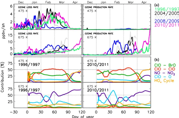
Figure 6a shows the ozone loss and production rates sim-ulated at 475 K and 675 K for selected Arctic winters, in-cluding 1996/1997 and 2010/2011. In 1996/1997, the ozone
loss was moderate and, therefore, loss rates of about 2– 3 ppbv sh−1 (parts per billion by volume/sunlit hours) are simulated from mid-February to mid-March at 475 K, as a result of significant ClO enhancements in this time period. In 2010/2011, the model simulates an atypical loss rate of 2– 4 ppbv sh−1in March and early April. It should be noted that
there are high loss rates in December and January 2010/2011 in the lower stratosphere at 475 K as a result of enhancement in ClO, as also shown by Manney et al. (2011), which is im-portant for the cumulative ozone loss of the winter. As ex-pected, there is no O3production in the lower stratosphere.
In the middle stratosphere, at 675 K (Fig. 6a), a loss rate of 2–5 ppbv sh−1is simulated in March–April in 1996/1997. On the other hand, in 2010/2011, large loss rates of about 4– 5 ppbv sh−1 in January and 13 ppbv sh−1 in mid-April are calculated by the model. No significant O3production was
found until mid-March in both winters, but episodically high production rates of about 5–7 ppbv sh−1 in 1996/1997 and 10–12 ppbv sh−1in 2010/2011 are estimated thereafter.
In most Arctic winters, as depicted in the figure, the loss rates show a maximum of about 3–5 ppbv sh−1in
mid-January, mid-February and late February/early March in warm (2008/2009), moderately cold (2007/2008) and cold (2004/2005) winters, respectively, and then suddenly drop to zero loss rate as there is no loss thereafter in the lower stratosphere, at 475 K. Though the loss rates are larger in late February–early March at higher altitudes (e.g. 675 K), O3production rates outweigh these high loss rates even in
cold winters. In contrast, there are higher ozone loss rates at 475 K in March and early April and relatively lower O3
production rates at 675 K in February through mid-March in 2010/2011 than in other years. This indicates that the winter
J. Kuttippurath et al.: Exceptional Arctic ozone loss in 2011 7079 × 107 km2 0.4 0.4 0.4 0.4 0.8 0.8 0.8 2010/2011 ECMWF A PSC 400 600 800 0 0.5 1 0.4 0.4 0.8 0.81.2 Mimosa−Chim ClO 400 600 800 0.4 0.4 0.8 1.2 Aura MLS ClO ppbv 0 0.5 1 1.5 3 3 3 6 6 6 9 9 12 Mimosa−Chim HNO 3 400 600 800 3 3 3 3 6 6 6 6 6 9 9 9 12 Aura MLS HNO 3 ppbv 0 10 121.5 1 2 2.5 3 3 3.5 4 4 4 4 4 5 Mimosa−Chim Ozone Potential Temperature (K) 400 600 800 11.5 1 2 2 2.5 3 3 3.5 4 4 4.5 5 Aura MLS Ozone ppmv 2 4 6 0.5 1 1 1 1.5 2 2 2
Mimosa−Chim Ozone Loss
Dec Jan Feb Mar Apr
−30 0 30 60 90 120 400 600 800 0.5 1 1 1 1.5
Aura MLS Ozone Loss ppmv
Day of year
Dec Jan Feb Mar Apr
0 30 60 90 1200
1 2
Fig. 5. Temporal evolution of the vertical distribution of ClO (second panel from the top), HNO3(third panel from the top), O3(fourth panel from the top), and ozone loss (bottom panel) from Mimosa-Chim and Aura MLS for the Arctic winter 2010/2011. The model fields are sampled at the location of MLS observations for each measurement inside the vortex and then averaged for the corresponding day. Both data
are smoothed for seven days. The Model and MLS ClO coincident profiles are selected for solar zenith angles <89◦and local time between
10 h and 16 h. The MLS ClO profiles are bias corrected (see text). The APSCcomputed from the ECMWF operational analyses is also shown
(top panel). The white dotted lines represent 475 K and 675 K. The blue/red colors show relatively low/high values of PSC areas or mixing
ratios of ClO, HNO3, O3, and ozone loss.
2010/2011 was unique in terms of the record ozone loss rates in the lower stratosphere in the March–April period.
We have also evaluated the contribution of various chem-ical cycles to the ozone loss in the lower and middle strato-sphere, as done by Kuttippurath et al. (2010b); results are shown in Fig. 6b. The general features and contributions from various chemical cycles in the lower and middle strato-sphere are consistent with those of previous studies (Kuttip-purath et al., 2010b; Vogel et al., 2008; Butz et al., 2007; Grooß et al., 2005; Hanson and Chipperfield, 1999; Woyke et al., 1999). However, in February–March 2011, our analy-ses show exceptional contributions from the ClO-ClO (30– 55%) and BrO-ClO (30–35%) cycles in terms of absolute values in the lower stratosphere at 475 K (although the rel-ative contributions from the various cycles look similar in both winters). The larger contributions of the halogen cy-cles in 2010/2011 are consistent with the prolonged appear-ance and large amounts of ClO during that period. In April 2011, a remarkable contribution from the HOx cycle (30–
50 %) is also calculated in the lower stratosphere. This is linked to relatively higher values of H2O and HNO3, the
sources of HOx in spring. In March–April 2011, the model
simulates comparatively higher abundances of NOx at
alti-tudes above 550 K (see Supplement figure), and hence this cycle dominates (with a 30–70 % contribution) the ozone loss there (Fig. 6b). The large contributions from these cycles in February–April are consistent with the large loss and loss rates during the period. The contributions of various chem-ical cycles during the winter 2010/2011 thus stand in con-trast to those in other Arctic winters (e.g. Kuttippurath et al., 2010b; Hanson and Chipperfield, 1999), as that winter exhibited stronger and more prolonged (February to April) chemical O3destruction in comparison to other Arctic
win-ters. Although the relative chemical cycle contributions (see Fig. 6b) in 1996/1997 are comparable to those in 2010/2011, these contributions from all cycles in absolute terms are pro-portional to the ozone losses that occurred in the respective winters (Kuttippurath et al., 2010b; Butz et al., 2007; Woyke et al., 1999). Further discussions on the contribution of var-ious cycles in the Arctic winter 1996/1997 can be found in Hanson and Chipperfield (1999). It should be borne in mind that the rate limiting step of these chemical cycles is the com-bination of O-atom with the specific molecule (e.g. O+NO2
7080 J. Kuttippurath et al.: Exceptional Arctic ozone loss in 2011
Fig. 6. (a) Vortex-averaged instantaneous ozone loss rates (left panel) and production rates (right panel) simulated by Mimosa-Chim at 475 K
and 675 K for the Arctic winter 1996/1997 (light green) and 2010/2011 (magenta) compared to those of 2004/2005 (black), 2007/2008 (grey), and 2008/2009 (blue). (b) Temporal evolution of the vortex-averaged contribution of the ClO-BrO (dark green), ClO-ClO (red), NO-NO2
(violet), ClO-O (light blue), and HOx(yellow) chemical cycles during the Arctic winter 1996/1997 (left panel) and 2010/2011 (right panel)
at 475 K and 675 K. The dotted horizontal lines represent 50 % of contribution and the vertical dotted lines mark the approximate boundaries of each month.
Fig. 6. (a) Vortex-averaged instantaneous ozone loss rates (left panel) and production rates (right panel) simulated by Mimosa-Chim at 475 K
and 675 K for the Arctic winter 1996/1997 (light green) and 2010/2011 (magenta) compared to those of 2004/2005 (black), 2007/2008 (grey),
and 2008/2009 (blue). (b) Temporal evolution of the vortex-averaged contribution of the ClO-BrO (dark green), ClO-ClO (red), NO-NO2
(violet), ClO-O (light blue), and HOx(yellow) chemical cycles during the Arctic winter 1996/1997 (left panel) and 2010/2011 (right panel)
at 475 K and 675 K. The dotted horizontal lines represent 50 % of contribution and the vertical dotted lines mark the approximate boundaries of each month.
duration of the contributions of these cycles and associated ozone loss in the middle stratosphere primarily depend on the available oxygen atoms in this altitude region.
Note that the loss of NOxhappens through
photodissocia-tion and thus in the absence of solar radiaphotodissocia-tion during the polar night, it is chemically long-lived. Therefore, its abundance in a particular winter is largely controlled by the prevailing me-teorology. When the polar vortex is very strong, large scale diabatic descent in the polar vortex can bring considerable amounts of NOxfrom higher altitudes (Solomon et al., 1982).
Strong descent of NOx was also observed during the
refor-mation of polar vortex after its split or displacement due to a major sudden stratospheric warming (MW). As discussed above, since the NOxcatalysed chemistry is very important
for the ozone loss at higher altitudes, the winters with larger mesospheric descent during MWs and solar proton events merit a special mention. For instance: studies report large scale NOx-rich airmass descent during MW of the Arctic
winter 2003/2004 and 2005/2006 (Randall et al., 2009), al-though the enhancement of stratospheric NOxin 2003/2004
was connected to solar proton events and associated excess production in the mesosphere (Vogel et al., 2008). Neverthe-less, both of these winters were prone to additional ozone loss in the middle and upper stratosphere due to higher NOx
abundances as reported by Vogel et al. (2008) and Kuttip-purath et al. (2010b). It has to be kept in mind that there were no MWs and large NOx influx from the mesosphere
in 1996/1997 and 2010/2011, and the contribution of NOx
is discussed with respect to the amount of NOx present in
2010/2011 in comparison to that of 1996/1997 only. There-fore, the interannual variability of NOx (and thus, the NOx
driven ozone loss) in the stratosphere depends on the dynam-ics of each winter.
3.4 Partial column ozone loss
To get a complete overview of the ozone loss, we have com-puted the partial column ozone loss in two potential tempera-ture ranges, 350–850 K and 350–550 K, from the MLS mea-surements inside the vortex and the corresponding Mimosa-Chim simulations (shown in Figs. 4 and 5). In 1996/1997, the Mimosa-Chim simulated partial column ozone loss at the UARS MLS sampling points over 350–550 K reaches 7 DU (Dobson Unit), 17 DU, and 44 DU in late January, late February and late April, respectively. The accumulated ozone loss from the model over 350–850 K by late April shows 62 DU. Identical values are also estimated from the UARS MLS measurements, about 43 DU over 350–550 K and 61 DU over 350–850 K by late April. These estimations
J. Kuttippurath et al.: Exceptional Arctic ozone loss in 2011 7081
18 J. Kuttippurath et al.: Exceptional Arctic ozone loss in 2011
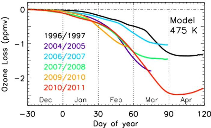
Fig. 7. Vortex-averaged ozone loss simulated by Mimosa-Chim
for the Arctic winters 1996/1997 (black), 2004/2005 (violet), 2006/2007 (blue), 2007/2008 (green), 2009/2010 (yellow), and 2010/2011 (red) at 475 K. The dotted vertical lines mark approx-imate boundaries of each month and the dash-dotted horizontal line is 0 ppmv.
are close to the findings of Tilmes et al. (2006) and Harris et al. (2010), who report about 61 ± 20 DU from satellite and 50 ± 20 DU from ozonesonde measurements, respectively, over 380–550 K. The total column ozone loss simulated with REPROBUS, about 50–60 DU (Lef`evre et al., 1998), is also comparable to our estimations. However, these estimations are significantly smaller than the total column ozone loss computed from ozonesonde observations by Knudsen et al. (1998), and Terao et al. (2002), of about 79–96 DU. This off-set could be due to the differences in the model simulations, vortex edge criterion, ozone loss estimation method and data used for the loss computations in the respective studies.
In 2010/2011, the partial column ozone loss simulated by Mimosa-Chim at the Aura MLS footprints reaches about 6 DU, 20 DU, 62 DU, and 112 DU by the end of each month from December through March, and 148 DU in mid-April over 350–550 K. The maximum ozone loss estimated for the 350–850 K altitude range is slightly higher, about 160 DU in mid-April, consistent with the loss simulated above 550 K. The Aura MLS observations show an analogous progression of ozone depletion with time for both column ranges, but the maximum loss is slightly lower than the simulated one, about 115 DU at 350–550 K and 131 DU at 350–850 K. These dif-ferences are consistent with the bias found between the mea-sured and modeled ClO and O3. Nonetheless, these column
ozone loss estimations are in good agreement with those es-timated by Manney et al. (2011) from the Ozone Monitoring Instrument measurements on 26 March 2011 (∼140 DU to-tal column loss) and by Sinnhuber et al. (2011) from the MI-PAS observations by late March (∼120 DU at 380–550 K). The total column ozone loss calculated from the Multi-sensor Reanalysis by Balis et al. (2011) is about 95±8 DU (per-sonal communication) and is comparable to our estimations. The slight differences between various ozone loss estimates
Table 1. Vortex-averaged (≥65◦, Equivalent Latitude) partial col-umn ozone loss (DU) estimated over 350–850 K and 350–550 K from the MLS sampling inside the vortex and corresponding Mimosa-Chim simulations. Here the winter 1996/1997 is 1997 and the same nomenclature procedure is also used for the other winters. The calculations for the moderately cold winter 2010 is done from 1 December to 28 February. The maximum loss is found (shown below) around late/mid-March in 2005, 2007, and 2008 and around late/mid-April in 1997 and 2011. 350–850 K 1997 2005 2007 2008 2010 2011 Mimosa-Chim 61 109 80 98 79 160 MLS 60 115 84 112 60 130 350–550 K Mimosa-Chim 42 91 57 80 55 140 MLS 41 81 62 90 42 115
can be due to the reasons discussed above (for the winter 1996/1997). However, the difference with Balis et al. (2011) could be due to the differences in vortex area calculations, as they use a vortex edge criterion of 70◦N Equivalent Lat-itude at 475 K, but we consider the vortex criterion at each altitude. This is particularly important as they use total col-umn ozone data. In addition, their passive tracer simulation is slightly different from that shown in other studies. Note also that model differences or inaccuracies in passive tracer calculations can significantly affect the loss values. For in-stance: ozone loss calculations based on a pseudo-tracer, in which only chlorine-activating heterogeneous reactions are turned off (Balis et al., 2011; Singleton et al., 2005), yield about 10–25% lower loss than that estimated in this study.
3.5 Comparison with other Arctic winters
Though ozone loss in the Arctic has been observed and esti-mated since 1989, there were only a few cold winters show-ing large ozone loss in the last two decades (e.g. Manney et al., 2011; Sonkaew et al., 2011; Kuttippurath et al., 2010b; WMO, 2007; Grooß et al., 2005; Goutail et al., 2005; Rex et al., 2004). A majority of the Arctic winters were warm (e.g. 2000/2001, 2003/2004, 2005/2006 and 2008/2009) or moderately cold (e.g. 1991/1992, 1993/1994, 1997/1998, 2006/2007, and 2007/2008), and therefore, the ozone loss es-timated from ground-based UV-visible total ozone measure-ments showed a loss of about 25–30 DU and 60 DU, respec-tively (WMO, 2011). The winters 1994/1995, 1995/1996, 1999/2000, and 2004/2005 were very cold with signifi-cant ozone loss of >80–90 DU (Kuttippurath et al., 2010b; Goutail et al., 2005). Note that a similar ozone depletion computation over 380–550 K from ozonesonde and satellite measurements is also available for each winter (WMO, 2011; Harris et al., 2010; Tilmes et al., 2006; Andersen and Knud-sen, 2002). Table 1 shows the partial column ozone loss over
two different altitude bounds for the recent cold/moderately cold Arctic winters. Compared to the other Arctic winters, the loss in 1996/1997 is on the scale of a moderately cold winter, i.e. 60–61 DU over 350–850 K. However, the loss es-timated for 2010/2011, 130–160 DU over 350–850 K, is un-doubtedly the largest among the Arctic winters, as the pre-vious maximum of 109–115 DU was in 2004/2005 (WMO, 2011; Kuttippurath et al., 2010b). Figure 7 also shows that the loss in 1996/1997 is moderate (1.2 ppmv) and the loss in 2010/2011 is the largest (2.4 ppmv) as compared to other winters. The ozone loss in 2004/2005 is somewhat larger than that of 2010/2011 in February–March, but the addi-tional loss of ∼0.8 ppmv thereafter, in March to mid-April 2011, is exceptional. Thus, our analyses confirm the results presented by Manney et al. (2011), who discuss ozone loss during several cold Arctic winters using ozone loss pro-files.
4 Comparison with the Antarctic scenario
Since the ozone loss in the Arctic winter 2010/2011 is un-precedented as analysed in this and previous studies (Man-ney et al., 2011; Sinnhuber et al., 2011), we compare the re-sults with the Antarctic ozone loss. Some additional model runs are performed for a few Antarctic winters and are com-pared to the Aura MLS observations. Though the main ozone loss processes are alike, the meteorology is entirely differ-ent in the two polar regions, giving rise to the difference be-tween the ozone loss observed in the respective polar regions (Solomon et al., 2007; WMO, 2007). On average, our anal-yses for various winters in 2004–2010 show that peak ozone loss (>2 ppmv) in the Antarctic stratosphere occurs over a broader altitude range of 350–650 K and usually shows its maximum in the late September and early October period. The peak ozone loss altitudes hardly change, but the maxi-mum loss usually varies between 2.5 ppmv and 3.5 ppmv, de-pending on the temperature history of each winter. The colder Antarctic winters such as 2006 show a peak loss of about 3.5 ppmv, while the warmer winters, like 2004 and 2009, ex-hibit a peak loss of about 2.5 ppmv over 450–550 K. In ad-dition, the total column ozone loss in the Antarctic winters usually shows about 130–150 DU in the warmer winters and about 160–180 DU in the colder winters (Kuttippurath et al., 2010a). It appears that the maximum partial column ozone loss estimated for the Arctic winter 2010/2011 in this study is close to the loss computed for the early years of Antarctic ozone depletion (1985–1991) (Manney et al., 2011; WMO, 2007) and the relatively warmer Antarctic winters (e.g. 2002, 2004, and 2009) (WMO, 2011, 2007; Manney et al., 2011; Kuttippurath et al., 2010a).
Figure 8 illustrates the vortex-averaged ClO and ozone loss estimated in the Arctic winter 2010/2011 and the mean vortex-averaged ozone loss estimated for the seven Antarc-tic winters: 2004–2010. We use the same model
Mimosa-Fig. 8. ClO (left) and ozone loss (right) profiles inside the
vor-tex from Mimosa-Chim (green) and MLS (red) in the Arctic win-ter 2010/2011, and the mean September and October ozone loss profiles in the Antarctic vortex averaged for seven winters (2004– 2010). The dotted vertical line is 1.8 ppbv of ClO or 2.5 ppmv of ozone loss. The dashed vertical line is 0 ppmv. The dotted horizon-tal lines are 475 K and 550 K.
Chim and model set-up (input data, chemistry and dynam-ics), Aura MLS measurements, and the passive method for the ozone loss calculations in the Antarctic to make a fair comparison with those in the Arctic. Note that the Antarc-tic measurements shown are the Aura MLS O3 v2.2, but
the Arctic observations are v3.3. However, the difference be-tween the vortex-averaged O3from v2.2 and v3.3 is
negligi-bly small and thus, we can robustly compare these values di-rectly. The ozone loss estimated in these Antarctic winters is about 2.5–3.2 ppmv in the model and 2.4–2.8 ppmv in Aura MLS. The ozone loss estimated in March/April of the Arc-tic winter 2010/2011 is comparable to that of the Septem-ber average in the Antarctic, as already shown by Manney et al. (2011). Nevertheless, the Arctic ozone loss is marginally smaller than that of the October average that includes three relatively warm (2004, 2009 and 2010) and two very cold (2006 and 2008) Antarctic winters. The altitudes of maxi-mum ozone loss of the 2010/2011 Arctic winter, 425–575 K, are also identical to those of the Antarctic winters. There-fore, in addition to the column ozone, the ozone loss pro-files in the Arctic winter 2010/2011 also show ozone loss features matching those found in the Antarctic stratosphere. The model simulates relatively lower O3than MLS for most
Antarctic winters and thus, modeled ozone loss (i.e. model O3– model tracer) is larger than the loss estimated with the
MLS measurements (i.e. MLS O3– model tracer).
In most Arctic winters the peak ozone loss is confined to the lower stratosphere centered around 450 K (e.g. Manney et al., 2011, 2003; Kuttippurath et al., 2010b; Rex et al., 2004).
J. Kuttippurath et al.: Exceptional Arctic ozone loss in 2011 7083
The loss above 550 K contributes about 19 ± 7 DU to the to-tal column loss, which is mainly driven by NOx catalyzed
chemistry in the middle stratosphere (Kuttippurath et al., 2010b). On the other hand, as shown by the ozone loss pro-files, ozone loss in the Antarctic stratosphere takes place over a broad altitude range centered around 550 K, and thus nearly half of the loss occurs above this isentropic level. Therefore, the Antarctic partial column (380–550 K) ozone loss (around 130 DU) computed by Tilmes et al. (2006) is not directly comparable to the partial column ozone loss estimated here for the Arctic winter 2010/2011. In addition, the sparse sam-pling of the Halogen Occultation Experiment in the southern polar vortex region, which does not always cover the maxi-mum ozone loss period of the Antarctic, makes the compari-son more difficult.
5 Conclusions
A comprehensive analysis of the Arctic winters 1996/1997 and 2010/2011 is presented with respect to the dynamical and chemical evolution of the winters. Both winters show a prolonged stable vortex from December to late April. However, the winter 1996/1997 was moderately cold during December–February and thus, occasional chlorine activation led to a moderate ozone loss of about 1.2 ppmv around 475– 550 K or 61 DU over 350–850 K by late March–late April. In contrast, the Arctic winter 2010/2011 experienced the largest area and longest period ever of chlorine activation, with ClO values up to 1.8 ppbv around 450–550 K, which translated to the record ozone loss of around 2.4 ppmv at the same altitudes in late-March/mid-April. The partial column esti-mates over 350–850 K also show a correspondingly massive loss of about 130–160 DU in mid-April. The simulated ozone loss rates show large values of 2–4 ppbv sh−1in March–early April at 475 K, which are uncommon in the Arctic at this time of the winter. In tune with these ozone loss features, the ClO-ClO and ClO-BrO cycles show increasingly larger val-ues (∼30–55 % and 30–35 %, respectively) in late February– March, as does the HOxcycle in April (about 30–50 %) in the
lower stratosphere, at 475 K. Additionally, significant ozone loss of about 0.7–1.2 ppmv is also computed at 550–700 K in March–April 2011. As expected, the NOx cycle dominates
the ozone destruction processes in the middle stratosphere, with a contribution of around 30–70 % at 675 K.
The ozone loss in the Arctic winter 2010/2011 is close to those estimated in the Antarctic winters, as assessed in this study and already shown by Manney et al. (2011). However, it has to be kept in mind that the ozone loss values in the Arc-tic winter 2010/2011 are comparable to those of the relatively warm Antarctic winters only, though September averages of the cold Antarctic winters also show similar magnitude of ozone loss. This is also applicable to total column ozone loss analyses as they show loss ranges (130–140 DU) equivalent to those of the warm Antarctic winters (e.g. 2004 and 2010)
and the early years of the Antarctic ozone depletion (1985– 1991), as discussed in Sect. 4. The atypically prolonged chlo-rine activation and large denitrification triggered this high ozone loss of 2.4 ppmv or 130–160 DU in 2010/2011. Fur-thermore, large loss (1.5 ppmv) over a broader altitude range (400–600 K) similar to that of the Antarctic is observed for the first time in the 2010/2011 Arctic winter. Nevertheless, since the halogens are decreasing slowly, the ozone loss in the polar stratosphere is expected to decrease even in cold winters. Yet, as discussed in Sinnhuber et al. (2011), with the predicted rate of stratospheric cooling in a climate changing world, the expected reduction in halogens may not help to cut down the ozone loss rates in very cold winters in the next decade. Therefore, cold winters of this kind with a similar range of ozone loss can be expected in the future (Manney et al., 2011; Sinnhuber et al., 2011).
Supplementary material related to this article is
available online at: http://www.atmos-chem-phys.net/12/ 7073/2012/acp-12-7073-2012-supplement.pdf.
Acknowledgements. The ECMWF data are taken from the
NADIR/NILU data base and are greatly acknowledged. J. K. thanks Cathy Boonne, IPSL, Paris for the REPROBUS model code for the simulations and Slimane Bekki and Marion Marchand for their support during this study. Participation of Jayanarayanan Kuttippurath and Franck Lef`evre in this work was supported by the European Commission as a part of the FP7 RECONCILE project under the Grant number: RECONCILE-226365-FP7-ENV-2008-1. Work at the Jet Propulsion Laboratory, California Institute of Technology, was done under contract to NASA.
Edited by: W. Lahoz
The publication of this article is financed by CNRS-INSU.
References
Andersen, S. B. and Knudsen, B. M.: The influence of vortex ozone depletion on Arctic ozone trends, Geophys. Res. Lett., 29, 2013, doi:10.1029/2001GL014595, 2002.
Balis, D., Isaksen, I. S. A., Zerefos, C., Zyrichidou, I., Eleftheratos, K., Tourpali, K., Bojkov, R., Rognerud, B., Stordal, F., Søvde, O. A., and Orsolini, Y.: Observed and Modelled record ozone decline over the Arctic during winter/spring 2011, Geophys. Res. Lett., 38, L23801, doi:10.1029/2011GL049259, 2011.
Burkholder, J. B., Orlando, J. J., and Howard, C. J.: Ultraviolet
ab-sorption cross-sections of Cl2O2 between 210 and 410 nm, J.
Phys. Chem., 94, 687–695, 1990.
Butz, A., B¨osch, H., Camy-Peyret, C., Dorf, M., Engel, A., Payan, S., and Pfeilsticker, K.: Observational constraints on the ki-netics of the ClO-BrO and ClO-ClO ozone loss cycles in the Arctic winter stratosphere, Geophys. Res. Lett., 34, L05801, doi:10.1029/2006GL028718, 2007.
Coy, L., Nash, E. R., and Newman, P. A.: Meteorology of the polar vortex: Spring 1997, Geophys. Res. Lett., 24, 2693–2696, 1997. Froidevaux, L., Jiang, Y. B., Lambert, A., Livesey, N. J., Read, W. G., Waters, J. W., Browell, E. V., Hair, J. W., Avery, M. A., McGee, T. J., Twigg, L. W., Sumnicht, G. K., Jucks, K. W., Margitan, J. J., Sen, B., Stachnik, R. A., Toon, G. C., Bernath, P. F., Boone, C. D., Walker, K. A., Filipiak, M. J., Harwood, R. S., Fuller, R. A., Manney, G. L., Schwartz, M. J., Daffer, W. H., Drouin, B. J., Cofield, R. E., Cuddy, D. T., Jarnot, R. F., Knosp, B. W., Perun, V. S., Snyder, W. V., Stek, P. C., Thurstans, R. P., Wagner, P. A.: Validation of Aura Microwave Limb Sounder stratospheric ozone measurements, J. Geophys. Res., 113, D15S20, doi:10.1029/2007JD008771, 2008. Goutail, F., Pommereau, J.-P., Lef`evre, F., van Roozendael, M.,
An-dersen, S. B., K˚astad Høiskar, B.-A., Dorokhov, V., Kyr¨o, E., Chipperfield, M. P., and Feng, W.: Early unusual ozone loss during the Arctic winter 2002/2003 compared to other winters, Atmos. Chem. Phys., 5, 665–677, doi:10.5194/acp-5-665-2005, 2005.
Grooß, J.-U., Konopka, P., and M¨uller, R.: Ozone chemistry dur-ing the 2002 Antarctic vortex split, J. Atmos. Sci., 62, 860–870, 2005.
Hanson, D. and Mauersberger, K.: Laboratory studies of the ni-tric acid trihydrate: implications for the south polar stratosphere, Geophys. Res. Lett., 15, 855–858, 1998.
Hanson, G. and Chipperfield, M.: Ozone loss at the edge of the polar vortex, J. Geophys. Res., 104, 1837–1845, 1999.
Harris, N. R. P., Lehmann, R., Rex, M., and von der Gathen, P.: A closer look at Arctic ozone loss and polar stratospheric clouds, Atmos. Chem. Phys., 10, 8499–8510, doi:10.5194/acp-10-8499-2010, 2010.
Hurwitz, M. M., Newman, P. A., and Garfinkel, C. I.: The Arctic vortex in March 2011: a dynamical perspective, Atmos. Chem. Phys., 11, 11447–11453, doi:10.5194/acp-11-11447-2011, 2011. Kleinb¨ohl, A., Bremer, H., K¨ullmann, H., Kuttippurath, J., Brow-ell, E. V., Canty, T., Salawitch, R. J., Toon, G. C., and Notholt, J.: Denitrification in the Arctic mid-winter 2004/2005 observed by airborne submillimeter radiometry, Geophys. Res. Lett., 32, L19811, doi:10.1029/2005GL023408, 2005.
Knudsen, B. M., Larsen, N., Mikkelsen, I. S., Morcrette, J.-J., Braa-then, G. O., Kyro, E., Fast, H., Gernandt, H., Kanzawa, H., Nakane, H., Dorokhov, V., Yushkov, V., Hansen, G., Gil, M., and Shearman, R. J.: Ozone depletion in and below the Arctic vortex for 1997, Geophys. Res. Lett., 25, 627–630, 1998.
Kondo, Y., H. Irie, M. Koike, and G. E. Bodeker: Denitri-fication and nitriDenitri-fication in the Arctic stratosphere during the winter of 1996–1997, Geophys. Res. Lett., 27, 337–340, doi:10.1029/1999GL011081, 2000.
Kuttippurath, J., Goutail, F., Pommereau, J.-P., Lef`evre, F., Roscoe, H. K., Pazmi˜no, A., Feng, W., Chipperfield, M. P., and Godin-Beekmann, S.: Estimation of Antarctic ozone loss from
ground-based total column measurements, Atmos. Chem. Phys., 10, 6569–6581, doi:10.5194/acp-10-6569-2010, 2010a.
Kuttippurath, J., Godin-Beekmann, S., Lef`evre, F., and Goutail, F.: Spatial, temporal, and vertical variability of polar stratospheric ozone loss in the Arctic winters 2004/2005–2009/2010, Atmos. Chem. Phys., 10, 9915–9930, doi:10.5194/acp-10-9915-2010, 2010b.
Lef`evre F., Figarol, F., Carslaw, K. S., and Peter, T.: The 1997 Arctic ozone depletion quantified from three-dimensional model simu-lations, Geophys. Res. Lett., 25, 2425–2428, 1998.
Livesey, N. J., Read, W. G., Froidevaux, L., Waters, J. W., Santee, M. L., Pumphrey, H. C., Wu, D. L., Shippony, Z., and Jarnot, R. F.: The UARS Microwave Limb Sounder version 5 data set: Theory, characterization, and validation, J. Geophys. Res., 108, 4378, doi:10.1029/2002JD002273, 2003.
Livesey, N. J., Read, W. G., Froidevaux, L., Lambert, A., Manney, G. L., Pumphrey, H. C., Santee, M. L., Schwartz, M. J., Wang, S., Cofeld, R. E., Cuddy, D. T., Fuller, Jarnot, R. F., Jiang, J. H., Knosp, B. W., Stek, P. C., Wagner, P. A., and Wu, D. L.: Earth Observing System (EOS) Aura Microwave Limb Sounder (MLS) Version 3.3 Level 2 data quality and description document, JPL D-33509, Jet Propulsion Laboratory California Institute of Tech-nology, Pasadena, California, USA, 91109–8099, 2011. Manney, G. L., Froidevaux, L., Santee, M. L., Zurek, R. W., and
Waters, J. W.: MLS observations of Arctic ozone loss in 1996– 1997, Geophys. Res. Lett., 24, 2697–2700, 1997.
Manney, G. L., Froidevaux, L., Santee, M., Livesey, N., Sabutis, J., and Waters, J.: Variability of ozone loss during Arc-tic winter (1991–2000) estimated from UARS Microwave Limb Sounder measurements, J. Geophys. Res., 108, 4149, doi:10.1029/2002JD002634, 2003.
Manney, G. L., Santee, M. L., Rex, M., Livesey, N. J., Pitts, M. C., Veefkind, P., Nash, E. R., Wohltmann, I., Lehmann, R., Froide-vaux, L., Poole, L. R., Schoeberl, M. R., Haffner, D. P., Davies, J., Dorokhov, V., Gernandt, H., Johnson, B., Kivi, R., Kyro, E., Larsen, N., Levelt, P. F., Makshtas, A., McElroy, C. T., Nakajima, H., Parrondo, M. C., Tarasick, D. W., von der Gathen, P., Walker, K. A., and Zinoviev, N. S.: Unprecedented Arctic ozone loss in 2011, Nature, 478, 469–475, doi:10.1038/nature10556, 2011. Papanastasiou, D. K., Papadimitriou, V. C., Fahey, D. W., and
Burkholder, J. B.: UV Absorption Spectrum of the ClO Dimer
(Cl2O2) between 200 and 420 nm, J. Phys. Chem. A, 113,
13711–13726, 2009.
Pitts, M. C., Thomason, L. W., Poole, L. R., and Winker, D. M.: Characterization of Polar Stratospheric Clouds with spaceborne lidar: CALIPSO and the 2006 Antarctic season, Atmos. Chem. Phys., 7, 5207–5228, doi:10.5194/acp-7-5207-2007, 2007. Randall, C. E., Harvey, V. L., Siskind, D. E., France, J., Bernath,
P. F., Boone, C. D., and Walker, K. A.: NOxdescent in the
Arc-tic middle atmosphere in early 2009, Geophys. Res. Lett., 36, L18811, doi:10.1029/2009GL039706, 2009.
Rex, M., Salawitch, R. J., von der Gathen, P., Harris, N. R. P., Chipperfield, M. P., and Naujokat, B.: Arctic ozone loss and climate change, Geophys. Res. Lett., 31, L04116, doi:10.1029/2003GL018844, 2004.
Sander, S., Friedl, R., Ravishankara, A., Golden, D., Kolb, C., Kurylo, M., Molina, M., Moortgat, G., Keller-Rudek, H., Finlayson-Pitts, B., Wine, P., Huie, R., and Orkin, V.: Chemical Kinetics and Photochemical Data for Use in Atmospheric
Stud-J. Kuttippurath et al.: Exceptional Arctic ozone loss in 2011 7085
ies (Evaluation Number 15), JPL Publication: 06–2, 2006. Santee, M. L., Manney, G. L., Froidevaux, L., Zurek, R. W., and
Wa-ters, J. W.: MLS observations of ClO and HNO3in the 1996–97
Arctic polar vortex, Geophys. Res. Lett., 24, 2713–2716, 1997. Santee, M. L., Manney, G. L., Froidevaux, L., Read, W. G., and
Wa-ters, J. W.: Six years of UARS Microwave Limb Sounder HNO3
observations: Seasonal, interhemispheric, and interannual vari-ations in the lower stratosphere, J. Geophys. Res., 104, 8225– 8246, 1999.
Santee, M. L., Lambert, A., Read, W. G., Livesey, N. J., Manney, G. L., Cofield, R. E., Cuddy, D. T., Daffer, W. H., Drouin, B. J., Froidevaux, L., Fuller, R. A., Jarnot, R. F., Knosp, B. W., Perun, V. S., Snyder, W. V., Stek, P. C., Thurstans, R. P., Wagner, P. A., Waters, J. W., Connor, B., Urban, J., Murtagh, D., Ricaud, P., Barrett, B., Kleinb¨ohl, A., Kuttippurath, J., K¨ullmann, H., von Hobe, M., Toon, G. C., and Stachnik, R. A.: Validation of the Aura Microwave Limb Sounder ClO measurements, J. Geophys. Res., 113, D15S22, doi:10.1029/2007JD008762, 2008. Shine, K. P.: The middle atmosphere in the absence of dynamical
heat fluxes, Q. J. Roy. Meteorol. Soc., 113, 603–633, 1987. Singleton, C. S., Randall, C. E., Chipperfield, M. P., Davies, S.,
Feng, W., Bevilacqua, R. M., Hoppel, K. W., Fromm, M. D., Manney, G. L., and Harvey, V. L.: 2002–2003 Arctic ozone loss deduced from POAM III satellite observations and the SLIM-CAT chemical transport model, Atmos. Chem. Phys., 5, 597– 609, doi:10.5194/acp-5-597-2005, 2005.
Sinnhuber, B.-M., Stiller, G. P., Ruhnke, R., von Clarmann, T., Kellmann, S., and Aschmann, J.: Arctic winter 2010/2011 at the brink of an ozone hole, Geophys. Res. Lett., 38, L24814, doi:10.1029/2011GL049784, 2011.
Solomon, S., Crutzen, P. J., and Roble, R. G.: Photochemical cou-pling between the thermosphere and the lower atmosphere: 1. Odd nitrogen from 50 to 120 km, J. Geophys. Res., 87, 7206– 7220, 1982.
Solomon, S., Portmann, R. W., and Thompson, D. W. J.: Contrasts between Antarctic and Arctic ozone depletion, P. Natl. Acad. Sci. USA, 104, 445–449, 2007.
Sonkaew, T., von Savigny, C., Eichmann, K.-U., Weber, M., Rozanov, A., Bovensmann, H., and Burrows, J. P.: Chemical ozone loss in Arctic and Antarctic polar winter/spring season de-rived from SCIAMACHY limb measurements 2002–2009, At-mos. Chem. Phys. Discuss., 11, 6555–6599, doi:10.5194/acpd-11-6555-2011, 2011.
Stimpfle, R. M., Wilmouth, D. M., Salawitch, R. J., and Anderson, J. G.: First measurements of ClOOCl in the stratosphere: the cou-pling of ClOOCl and ClO in the Arctic polar vortex, J. Geophys. Res., 109, D03301, doi:10.1029/2003JD003811, 2004
Terao, Y., Sasano, Y., Nakajima, H., Tanaka, H., and Yasunari, T.: Stratospheric ozone loss in the 1996/1997 Arctic winter: Evaluation based on multiple trajectory analysis for double-sounded air parcels by ILAS, J. Geophys. Res., 107, 8210, doi:10.1029/2001JD000615, 2002.
Tilmes, S., M¨uller, R., Engel, A., Rex, M., and Russell III, J.: Chemical ozone loss in the Arctic and Antarctic stratosphere between 1992 and 2005, Geophys. Res. Lett., 33, L20812, doi:10.1029/2006GL026925, 2006.
Tripathi, O. P., Godin-Beekmann, S., Lef`evre, F., Marchand, M., Pazmi˜no, A., Hauchecorne, A., Goutail, F., Schlager, H., Volk, C. M., Johnson, B., Konig-Langlo, G., Balestri, S., Stroh, F., Bui, T. P., Jost, H. J., Deshler, T., and von der Gathen, P.: High resolution simulation of recent Arctic and Antarctic stratospheric chemical ozone loss compared to observations, J. Atmos. Chem., 55, 205– 226, doi:10.1007/s10874-006-9028-8, 2006.
Vogel, B., Konopka, P., Grooß, J.-U., M¨uller, R., Funke, B., L´opez-Puertas, M., Reddmann, T., Stiller, G., von Clarmann, T., and Riese, M.: Model simulations of stratospheric ozone loss caused
by enhanced mesospheric NOxduring Arctic Winter 2003/2004,
Atmos. Chem. Phys., 8, 5279–5293, doi:10.5194/acp-8-5279-2008, 2008.
Woyke, T., M¨uller, R., Stroh, F., McKenna, D. S., Engel, A., Margi-tan, J. J., Rex, M., and Carslaw, K. S.: A test of our understanding of the ozone chemistry in the Arctic polar vortex based on in situ
measurements of ClO, BrO, and O3in the 1994/1995 winter, J.
Geophys. Res., 104, 18755–18768, 1999.
WMO (World Meteorological Organisation): Scientific assessment of ozone depletion: 2006, Global Ozone Research and Monitor-ing Project-Report No. 50, 572 pp., Geneva, Switzerland, 2007. WMO (World Meteorological Organisation): Scientific assessment
of ozone depletion: 2006, Global Ozone Research and Monitor-ing Project-Report No. 52, 516 pp., Geneva, Switzerland, 2011. Woods, A.: Medium-Range Weather Prediction - the European