HAL Id: hal-02458612
https://hal.archives-ouvertes.fr/hal-02458612
Submitted on 26 Jun 2020
HAL is a multi-disciplinary open access
archive for the deposit and dissemination of
sci-entific research documents, whether they are
pub-lished or not. The documents may come from
teaching and research institutions in France or
abroad, or from public or private research centers.
L’archive ouverte pluridisciplinaire HAL, est
destinée au dépôt et à la diffusion de documents
scientifiques de niveau recherche, publiés ou non,
émanant des établissements d’enseignement et de
recherche français ou étrangers, des laboratoires
publics ou privés.
Mercury’s low-degree geoid and topography controlled
by insolation-driven elastic deformation
N. Tosi, O. Čadek, M. Běhounková, M. Káňová, A.-c. Plesa, M. Grott, D.
Breuer, S. Padovan, M. Wieczorek
To cite this version:
N. Tosi, O. Čadek, M. Běhounková, M. Káňová, A.-c. Plesa, et al.. Mercury’s low-degree geoid
and topography controlled by insolation-driven elastic deformation. Geophysical Research Letters,
American Geophysical Union, 2015, 42 (18), pp.7327-7335. �10.1002/2015GL065314�. �hal-02458612�
Mercury’s low-degree geoid and topography controlled
by insolation-driven elastic deformation
N. Tosi1,2, O. ˇCadek3, M. B ˇehounková3, M. Ká ˇnová3, A.-C. Plesa2, M. Grott2, D. Breuer2, S. Padovan2, and M. A. Wieczorek4
1Department of Astronomy and Astrophysics, Technische Universität Berlin, Berlin, Germany,2Department of Planetary
Physics, German Aerospace Center, Berlin, Germany, 3Department of Geophysics, Charles University, Prague, Czech
Republic,4Institut de Physique du Globe de Paris, Sorbonne Paris Cité, Université Paris Diderot, Paris, France
Abstract
Mercury experiences an uneven insolation that leads to significant latitudinal and longitudinal variations of its surface temperature. These variations, which are predominantly of spherical harmonic degrees 2 and 4, propagate to depth, imposing a long-wavelength thermal perturbation throughout the mantle. We computed the accompanying density distribution and used it to calculate the mechanical and gravitational response of a spherical elastic shell overlying a quasi-hydrostatic mantle. We then compared the resulting geoid and surface deformation at degrees 2 and 4 with Mercury’s geoid and topography derived from the MErcury, Surface, Space ENvironment, GEochemistry, and Ranging spacecraft. More than 95% of the data can be accounted for if the thickness of the elastic lithosphere were between 110 and 180 km when the thermal anomaly was imposed. The obtained elastic thickness implies that Mercury became locked into its present 3:2 spin orbit resonance later than about 1 Gyr after planetary formation.1. Introduction
The long-wavelength gravity field and topography of terrestrial bodies are generally interpreted in terms of lateral heterogeneities of the crust-mantle interface [e.g., Wieczorek, 2015], of deep-seated density anomalies due to mantle convection, and of the accompanying dynamic topography of compositional interfaces [e.g.,
Redmond and King, 2007], or a combination thereof. The degree 2 coefficients of Mercury’s gravity field and
shape have long been known to depart significantly from hydrostatic equilibrium [Anderson et al., 1987, 1996]. The constraints on the degree 2 gravity obtained from Mariner 10 flybys, in combination with measurements of equatorial ellipticity form radar ranging, have been first used by Anderson et al. [1996] to infer a crustal thickness of 200 ± 100 km under the assumption that the topography is Airy compensated. These values, however, are considerably larger than those obtained from subsequent estimates based on topographic relax-ation models, which favor the lower end of this range [Watters and Nimmo, 2010], and on recent models based on gravity and topography data of the MErcury, Surface, Space ENvironment, GEochemistry, and Ranging (MESSENGER) spacecraft that yield values of few tens of kilometers only [James et al., 2015; Padovan et al., 2015]. In particular, Padovan et al. [2015] carried out an analysis of the geoid-to-topography ratio (GTR) of the ancient terrane of Mercury’s northern hemisphere showing that, at spherical harmonics degrees 9≤ 𝓁≤15, the GTR is well explained by an Airy model of isostatic compensation with a mean crustal thickness of 35 ± 18 km. At longer wavelengths, for𝓁 ≤ 8, the GTR is significantly higher and scattered, suggesting that different mechanisms are needed to interpret this part of the spectrum [see also James et al., 2015]. The power spectra of Mercury’s dynamic geoid and topography obtained from 3-D spherical mantle convection models turn out to be much smaller than the observed ones [Padovan et al., 2015], indicating that, even if mantle convection were still ongoing, its signal would be too weak to be detected in the geoid and topography data, let alone to affect the longest wavelengths of these two fields.
Matsuyama and Nimmo [2009] analyzed Mercury’s gravity field resulting from additional effects: tidal
defor-mation, despinning, variable eccentricity, and reorientation of a residual bulge. They concluded that neither the mass excess associated with the Caloris basin nor a large remnant bulge acquired when the planet was rotating faster can account alone for the observed gravity at degree 2. They proposed instead a more complex scenario in which a (sufficiently) large gravity anomaly associated with Caloris drove the reorienta-tion of an also large remnant bulge through an event of true polar wander.
RESEARCH LETTER
10.1002/2015GL065314Key Points:
• Mercury’s shape and geoid explained by deformation due to deep, insolation-driven density anomalies • Elastic thickness between 110 and
180 km when the surface temperature anomaly was imposed
• 3:2 spin orbit resonance acquired later than about 1 Gyr after planetary formation Supporting Information: • Supporting Information S1 Correspondence to: N. Tosi, [email protected] Citation:
Tosi, N., O. ˇCadek, M. B ˇehounková, M. Ká ˇnová, A.-C. Plesa, M. Grott, D. Breuer, S. Padovan, and M. A. Wieczorek (2015), Mercury’s low-degree geoid and topography controlled by insolation-driven elastic deformation, Geophys. Res. Lett.,
42, doi:10.1002/2015GL065314.
Received 10 JUL 2015 Accepted 25 AUG 2015
Accepted article online 1 SEP 2015
©2015. American Geophysical Union. All Rights Reserved.
Geophysical Research Letters
10.1002/2015GL065314
Figure 1. (a) Distribution of Mercury’s surface temperature according to Vasavada et al. [1999] (see section 1 in Text S1). (b) Long-wavelength geoid and (c) topography from MESSENGER data. The three fields are plotted up to degree and order 4.
An alternative explanation for the low-degree gravity and topography of Mercury is offered by the peculiar pattern of its mean surface temperature and its accompanying consequences on the density distribution of the deep interior [Phillips et al., 2014]. Because of its 3:2 spin orbit resonance, high orbital eccen-tricity, and small obliquity, Mercury’s surface experiences an uneven insolation that not only leads to large latitudinal differences in temperature but also to sig-nificant longitudinal variations resulting in equatorial hot and cold regions form-ing so-called hot poles at 0∘ and 180∘ and warm poles at ±90∘ longitude (Figure 1a). The main part of the power spectrum of the surface temperature distribution is concentrated at degrees 2 (84%) and 4 (10%). Figures 1b and 1c show Mercury’s long-wavelength geoid and shape up to degree and order 4 obtained from the spherical harmonic model HGM005 of the gravitational potential [Mazarico
et al., 2014] and from a spherical
har-monic representation of the topography [Neumann, 2014]. Hot equatorial (cold polar) poles correlate with highs (lows) of the geoid and topography. Indeed, the degrees 2 and 4 account for a significant part of the power spectrum of the two fields: respectively, 76% and 7% of the geoid and 40% and 4% of the topog-raphy. Here we explore the correlation between insolation, geoid, and topog-raphy by investigating the mechanical and gravitational response of the litho-sphere and mantle to the internal thermal heterogeneities induced by the surface temperature distribution.
2. Methods
2.1. Thermal Evolution Model
We used the mantle convection code GAIA [Hüttig et al., 2013] to run a represen-tative 3-D simulation of Mercury’s thermal evolution using the same approach as in Tosi et al. [2013]. This model reflects a typical evolution scenario sat-isfying several constraints imposed by MESSENGER observations, including the prediction of a limited global contraction [Byrne et al., 2014]. We considered a 400 km thick silicate shell [Hauck et al., 2013] whose top 30 km consists of a fixed crust enriched in radiogenic heat sources with respect to the mantle according to a constant factor (Λ), with the concentration of U, Th, and K reflecting the observed surface abundances inferred from gamma ray spectroscopy [Peplowski et al., 2012]. Note that the parameter Λ (set to 2.7 in this simulation as in the nominal model presented by Tosi et al. [2013]) lies within the range of values for which evolution models are compatible with MESSENGER constraints, i.e., between 2.5 and 4.5 [Tosi et al., 2013]. Besides solving the
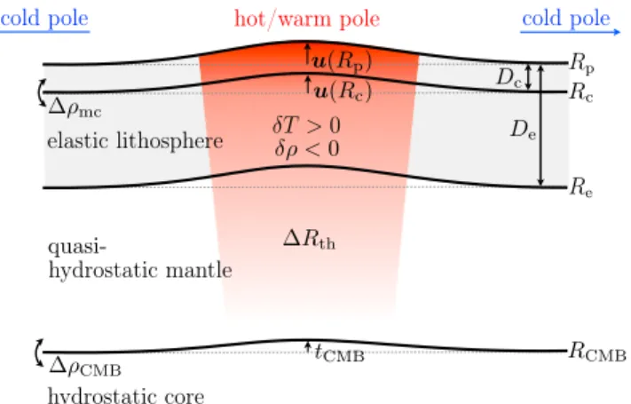
Figure 2. Schematic diagram of the elastic model used to calculate topography and geoid due to internal loading associated with temperature anomalies𝛿T(and hence density anomalies𝛿𝜌) induced by surface temperature variations and mantle convection.Rp,Rc,Re, andRCMBdenote the radii of the planet, crust (of thicknessDc), base of the elastic layer (of thicknessDe), and CMB;Δ𝜌mcandΔ𝜌CMBare density contrasts across the crust-mantle interface and CMB; u(Rp)andu(Rc)refer to the elastic displacements of the surface and crust-mantle interface, whiletCMBrepresents the deformation of the CMB;ΔRthis the displacement caused by density anomalies located below the elastic layer that cause thermal expansion or contraction of the mantle (see section 2 in Text S1 for details).
conservation equations of mass, momentum, and thermal energy under the extended Boussinesq approxi-mation [Christensen and Yuen, 1985], the model accounts for core cooling [e.g., Steinbach and Yuen, 1994] and decaying radiogenic heat sources as appropriate for thermal evolution models. Table S2 of the supporting information contains a list of all model parameters.
The major difference with respect to the models presented by Tosi et al. [2013] is that here, instead of consider-ing a uniform surface temperature, we employed as boundary condition the distribution shown in Figure 1a. This corresponds to that predicted by model TWO of Vasavada et al. [1999] whose details are discussed in section 1 in Text S1 of the supporting information. Although different scenarios have been proposed to explain how and when Mercury reached its current orbital resonance [Correia and Laskar, 2004; Wieczorek
et al., 2012; Noyelles et al., 2014], we simply assumed the pattern of Figure 1a to be constant. The implications
of this assumption will be discussed in sections 3 and 4. 2.2. Elastic Model
To evaluate the mechanical and gravitational response of the mantle to internal loads, we calculated the distribution of temperature anomalies𝛿T from the thermal evolution model:
𝛿T(r, 𝜗, 𝜑) = T(r, 𝜗, 𝜑) − ⟨T(r)⟩, (1)
where (r, 𝜗, 𝜑) denote radius, colatitude, and longitude, respectively, T(r, 𝜗, 𝜑) is the actual three-dimensional temperature field, and⟨T(r)⟩ its laterally averaged profile. We then used the obtained thermal anomalies to compute the mechanical response of the mantle using the spherical shell model sketched in Figure 2. The model consists of an elastic layer of thickness De, in which the momentum and continuity equations for an elastic, compressible, and self-gravitating continuum are solved in the spectral domain [Golle et al., 2012]. This elastic shell is partially composed of a crust of thickness Dc, across which a density contrast Δ𝜌mcis pre-scribed, and overlies a quasi-hydrostatic layer where shear stresses are neglected but whose deformation ΔRthcaused by thermal expansion and contraction is taken into account in the surface boundary conditions. The core-mantle boundary (CMB), across which a density jump Δ𝜌CMBis prescribed, is assumed to follow an equipotential, and its shape tCMBis also taken into account in the boundary conditions. The surface topog-raphy results from the elastic deformation of the surface u(Rp), from the expansion and contraction of the elastic lithosphere and deep mantle, and from the CMB topography. Internal temperature anomalies𝛿T along with the displacements of the surface, crust-mantle interface, and CMB are then employed to calculate in the spectral domain the gravitational potential at the surface and hence the geoid. Section 2 in Text S1 and Table S3 of the supporting information contain a detailed description of the conservation equations, boundary conditions, and parameters used.
Geophysical Research Letters
10.1002/2015GL065314
Figure 3. (a) Profiles of the minimum (blue), average (black), and maximum (red) mantle temperature from the 3-D thermal evolution model. Solid lines refer to the convective solution after 1 Gyr and dashed lines to the conductive solution after 4.5 Gyr. (b) Variance reduction as a function of elastic thickness for geoid and topography together (black) and separately (red and blue). Solid and dashed lines refer to the convective and conductive solutions.
3. Results
We first ran the 3-D thermal evolution model described in section 2.1. The parameters used here lead to the cessation of convection after about 3.5 Gyr. By monitoring the evolution of the temperature profiles beneath the hot and cold surface poles, we estimated that in about 500 Myr the pattern of surface temperature dif-fuses down to the CMB, reaching a quasi steady state that is maintained until the present day. This causes the formation of a long-wavelength temperature perturbation that reflects the surface distribution but does not interfere with the convection planform, which remains small-scale as in simulations employing a uniform sur-face temperature. Figure 3a shows laterally averaged profiles of the minimum, average, and maximum mantle temperature after 1 Gyr and 4.5 Gyr of evolution, respectively. The former correspond to a time at which the mantle was convecting and the transient signal due to the laterally varying temperature boundary conditions was well in a quasi steady state; the latter correspond to the present day, after the mantle became conduc-tive (see Figure S1 of the supporting information for a plot of the mantle temperature distribution at these two times.)
We then used the corresponding distribution of temperature anomalies as internal load for the elastic model described in section 2.2 to compute the resulting geoid and topography. Hot equatorial poles (Figure 1a) are associated with a positive geoid and topography (Figures 1b and 1c). The underlying lithosphere and mantle, being hotter than average, are characterized by a negative density anomaly, which, in absence of deformation, would lead to a negative geoid, in contrast with the observations. This negative geoid, however, can be compensated through the effect of positive density anomalies associated with a sufficiently large
upward deflection of the surface and CMB that largely depends on the thickness Deof the elastic lithosphere (the opposite argument clearly applies to cold poles and their geoid and topography lows).
In order to evaluate the agreement between models and observations, we performed a parameter space search by running several forward models using different elastic layer thicknesses. For every value of De, we computed the resulting variance reductionN,H(De) for the joint prediction of geoid (N) and topography (H) [e.g., Mitrovica and Forte, 1997]:
N,H(De) = [ 1 − ( aN ∑ 𝓁m ( Nmod 𝓁m (De) − Nobs𝓁m )2 ∑ 𝓁m ( Nobs 𝓁m )2 + aH ∑ 𝓁m ( Hmod 𝓁m (De) − Hobs𝓁m )2 ∑ 𝓁m ( Hobs 𝓁m )2 )] × 100%, (2)
where the sums only include𝓁 = 2 and 4; m = −𝓁, … , 𝓁, N𝓁mand H𝓁mare harmonic coefficients of the modeled (mod) and observed (obs) geoid and topography, respectively, and aN= aH= 1∕2. For the variance
reductionN(De) of the geoid alone, we set aN= 1 and aH= 0 in equation (2) and vice versa for the variance
reductionH(De) relative to the topography. Note that because of the symmetry of the surface temperature distribution (see Figure 1a and Table S1), spherical harmonic coefficients of odd degree and/or order of the modeled fields are negligible.
In Figure 3b, for both the convective and conductive solutions, we show the variance reductionsN,H(black), N(red), andH(blue), obtained using a model with a thermal expansivity𝛼 = 3 × 10⁻⁵K−1, Dc = 30 km, Δ𝜌mc= 500 kg m−3, and Δ𝜌
CMB= 3600 kg m−3. For values of Debetween ∼130 km and 140 km,N,Hshows a
pronounced peak of about 96%, with a sharp decrease away from these values. Note that negative values of are indicative of modeled geoid and/or topography that are anticorrelated with respect to the observations. The shape ofN,His very similar to that ofN; the shape ofHalso exhibits a maximum, which is attained for
an elastic thickness of ∼145 km. This maximum, however, is not as sharp as the one that characterizesN. In
particular, the variance reduction remains above 80% for values of Degreater than ∼145 km. The influence of the mode of heat transport on the estimate of Deis minor: the maxima of are attained at approximately the same value of Defor both the convective and conductive solutions. Indeed, the elastic model we used to calculate geoid and topography is insensitive to the absolute mantle temperature and only depends on density anomalies. These anomalies in turn, at degrees 2 and 4, are controlled by the distribution of surface temperature and are not affected by the presence of mantle convection, which is characterized by small-scale cells that do not perturb the long-wavelength signal generated by the insolation pattern.
Besides the thickness of the elastic shell, the thermal expansivity is the parameter that has the largest influence on the prediction of the data. As shown in Figure S2a, the maximum ofN,Hoccurs for De= 120, 130, or 165 km when assuming a convective mantle and𝛼 = 2.5, 3, or 3.5 × 10⁻⁵K−1, respectively (note that the conductive solution is again very similar to the convective one as shown in Figure S2b). Different values of the crustal thickness, which simply controls the depth at which the density contrast Δ𝜌mcis imposed, also affect the estimate of the elastic thickness, though to a lesser extent: the difference in the values of Deat which the maximum ofN,His attained is only ∼15 km for crustal thicknesses between 20 and 40 km (compare the solid, dashed, and dotted lines in Figure S2). Furthermore, as the CMB topography calculated with our model is typically small (few tens of meters at most), the density contrast between mantle and core plays only a negligible role.
Since the above estimates of the elastic thickness are independent of the absolute mantle temperature, the best fitting value of Deis only indicative of the time at which the surface thermal anomaly propagated through the mantle and reached a quasi steady state (∼500 Myr after the planet was locked into the 3:2 resonance). Depending on the choice of the thermal expansivity and limiting us to consider only maxima ofN,H, the degrees 2 and 4 of geoid and topography are equally well predicted by our model when Delies approximately between 110 and 180 km (Figure S2).
In order to verify whether this range is compatible with estimates based on a more detailed rheological description of the mantle, which does depend on temperature, we employed the strength envelope formal-ism [McNutt et al., 1988] to provide an independent estimate of the elastic thickness. Under the assumption of small curvature, which is justified at the long wavelengths that we are considering [Grott and Breuer, 2010], we calculated Deas the mechanical thickness of the lithosphere, i.e., the depth corresponding to the
Geophysical Research Letters
10.1002/2015GL065314
Figure 4. Elastic thickness obtained using the strength envelope formalism for the temperature distribution corresponding (a) to the convective solution after 1 Gyr and (b) to the present-day conductive solution. (c) Time evolution of the minimum (dotted lines), average (solid lines), and maximum (dashed lines) elastic thicknessDe for three different values of the strain rate ̇𝜖. The gray area indicates the range ofDeobtained from the inversion of geoid and topography data.
temperature Tdat which the lithosphere loses its mechanical strength because of ductile flow [e.g., Grott and Breuer, 2008]: Td= Q R [ log( 𝜎 nB ̇𝜖 )]−1 , (3)
where Q, B, and n are rheological parameters, R is the gas constant,𝜎 a bounding stress, and ̇𝜖 the strain rate (see Table S4 for the assumed values). In Figure 4, we show the resulting distribution of Deassuming a strain rate of 10−18s−1and using the temperature field corresponding to the convective solution after 1 Gyr and to the conductive solution at present day (Figures 4a and 4b, respectively), as well as the time evolution of the
minimum, average, and maximum Defor three different values of the strain rate (Figure 4c) that are represen-tative for terrestrial planets [McGovern et al., 2002]. Maxima and minima of De, corresponding to cold and hot poles, differ by ∼25 km in both the convective and conductive cases, in agreement with previous estimates of Williams et al. [2011] based on parametrized thermal evolution models. Furthermore, Figure 4a shows that the small-scale planform of mantle convection that characterizes Mercury’s thin mantle does not affect the long-wavelength thermal perturbation imposed by surface temperature variations (see also Figure S1). As illustrated in Figure 4c, because of mantle cooling, the mean elastic thickness increases significantly over time: from 85–100 km after 1 Gyr of evolution to 170–190 km at present day (depending on the choice of the strain rate). The results of our inversion of geoid and topography predict elastic thicknesses between ∼110 and 180 km. This range, marked in grey in Figure 4c, is consistent with the above estimates only after at least 1.5 Gyr. Since the time needed for the insolation pattern to propagate through the mantle and reach a quasi steady state is ∼500 Myr, this suggests that Mercury may have acquired its 3:2 spin orbit resonance relatively late in its evolution, about 1 Gyr after its formation or later.
4. Discussion
Both the low-degree geoid and topography can be naturally maintained out of equilibrium through deforma-tion of the elastic lithosphere and of the underlying mantle caused by deep, insoladeforma-tion-driven temperature anomalies, a mechanism also proposed by Phillips et al. [2014] in the framework of a simpler model of a conductive mantle with isostatically compensated topography. For an optimal choice of the thickness Deof the elastic lithosphere, our model reproduces well the observed geoid and topography at degrees 2 and 4 (Figure 3b). The best fitting value of Devaries between 110 and 180 km, chiefly depending on the choice of the coefficient of thermal expansion. Indeed, a topography that both fits the observed shape and allows us to reproduce the observed geoid is obtained using either a thick lithosphere and a small thermal expansiv-ity or, vice versa, a thin lithosphere and a large thermal expansivexpansiv-ity (Figure S2). Other parameters, such as the crustal thickness, the density contrast across the crust-mantle interface, or the CMB play a second-order role. The mechanical and gravitational responses of the lithosphere and mantle calculated with the above model do not depend on the absolute mantle temperature and are little influenced by the presence of convection. Our estimates of Deare thus only representative for the time at which the pattern of surface temperature developed through the mantle. Because of mantle cooling, however, the thickness of the lithosphere increases over time. We thus computed Deusing the strength envelope formalism [McNutt et al., 1988] and found that its average value increases from ∼85–100 km after 1 Gyr to ∼170–190 km at present day (Figure 4c). The above values can be reconciled with those predicted by the geoid and topography inversion (110–180 km) if Mercury was captured into its 3:2 spin orbit resonance after about 1 Gyr of evolution or later (Figure 4c). This scenario compares favorably with the one proposed by Wieczorek et al. [2012] according to which Mercury escaped from an initial synchronous rotation as a consequence of a large impact, allowing subse-quent capture into the present-day 3:2 resonance [see also Correia and Laskar, 2012]. The last such impact that could have accomplished this is the one that generated the Caloris basin at about 3.7 Ga. [Le Feuvre and
Wieczorek, 2011].
On the basis of the analysis of lobate scarps, Nimmo and Watters [2004] inferred elastic thicknesses of only 25–30 km at the time of faulting (about 4 Ga). These values are significantly lower than those predicted by our evolution model, i.e., between 75 and 90 km at that time. The latter range, however, is in good agreement with estimates of ∼75–125 km based on the analysis of tectonic structures related to Caloris [Melosh and
McKinnon, 1988].
The long-wavelength part of the spectrum of Mercury’s shape and gravity field possesses significant power also at degrees 3 and 5 [Mazarico et al., 2014; Neumann, 2014]. However, since the surface temperature dis-tribution is symmetric with respect to the equator and the small-scale thermal structures associated with mantle convection are uniformly distributed and do not provide a significant dynamic contribution [Padovan
et al., 2015], our model can only explain the degrees 2 and 4 of the two fields. Finding suitable mechanisms
accounting for these degrees remains a task for future models. Vast volcanic plains are concentrated in the northern hemisphere of the planet [e.g., Head et al., 2011], and a north-south asymmetry in the mantle den-sity distribution could thus arise as a consequence of compositionally distinct materials associated with the source regions of the partial melts that led to the formation of these plains. This density distribution could potentially induce a gravity response involving odd degrees. Large-scale impacts such as the one associated
Geophysical Research Letters
10.1002/2015GL065314
with the formation of Caloris [Roberts and Barnouin, 2012] or the effects of a residual mantle resulting from the crystallization of a magma ocean [Brown and Elkins-Tanton, 2009; Charlier et al., 2013] also represent viable options that will ultimately have to be verified quantitatively.5. Conclusions
The large latitudinal and longitudinal variations of Mercury’s surface temperature, which are predominantly of spherical harmonic degrees 2 and 4, induce at these same degrees a thermal perturbation throughout the mantle. Such perturbation causes a surface deformation and a geoid that are strongly influenced by the thick-ness of the elastic lithosphere and by the thermal expansion coefficient of the mantle. Using a 3-D thermal evolution model to calculate the temperature distribution in the mantle and lithosphere and a 3-D elastic model to compute their mechanical and gravitational responses, we showed that, for an elastic thickness De between ∼110 and 180 km, our model can predict the observed degrees 2 and 4 of the geoid and topogra-phy with a variance reduction of more than 95%. On the basis of independent estimates obtained with the strength envelope formalism applied to the evolution of the interior temperature, the above values can be accounted for if Mercury was trapped in its 3:2 resonance later than about 1 Gyr after planetary formation.
References
Anderson, J. D., G. Colombo, P. B. Esposito, E. L. Lau, and G. B. Trager (1987), The mass, gravity field, and ephemeris of Mercury, Icarus, 71(3), 337–349.
Anderson, J. D., R. F. Jurgens, E. L. Lau, M. A. Slade, and G. Schubert (1996), Shape and orientation of Mercury from radar ranging data, Icarus,
124(2), 690–697.
Brown, S. M., and L. T. Elkins-Tanton (2009), Compositions of Mercury’s earliest crust from magma ocean models, Earth Planet. Sci. Lett., 286, 446–455.
Byrne, P. K., C. Klimczak, A. M. C. ˙Sengör, S. C. Solomon, T. W. Watters, and S. A. Hauck (2014), Mercury’s global contraction much greater than earlier estimates, Nat. Geosci., 7(4), 301–307.
Charlier, B., T. L. Grove, and M. T. Zuber (2013), Phase equilibria of ultramafic compositions on Mercury and the origin of the compositional dichotomy, Earth Planet. Sci. Lett., 363, 50–60, doi:10.1016/j.epsl.2012.12.021.
Christensen, U. R., and D. Yuen (1985), Layered convection induced by phase transitions, J. Geophys. Res., 90(B12), 10,291–10,300. Correia, A. C. M., and J. Laskar (2004), Mercury’s capture into the 3/2 spin-orbit resonance as a result of its chaotic dynamics, Nature,
429(6994), 848–850.
Correia, A. C. M., and J. Laskar (2012), Impact cratering on Mercury: Consequences for the spin evolution, Astrophys. J. Lett., 751, L43, doi:10.1088/2041-8205/751/2/L43.
Golle, O., C. Dumoulin, G. Choblet, and O. ˇCadek (2012), Topography and geoid induced by a convecting mantle beneath an elastic lithosphere, Geophys. J. Int., 189(1), 55–72.
Grott, M., and D. Breuer (2008), The evolution of the Martian elastic lithosphere and implications for crustal and mantle rheology,
Icarus, 193(2), 503–515.
Grott, M., and D. Breuer (2010), On the spatial variability of the Martian elastic lithosphere thickness: Evidence for mantle plumes?,
J. Geophys. Res., 115, E03005, doi:10.1029/2009JE003456.
Hauck, S., et al. (2013), The curious case of Mercury’s internal structure, J. Geophys. Res. Planets, 118, 1204–1220, doi:10.1002/jgre.20091. Head, J., et al. (2011), Flood volcanism in the northern high latitudes of Mercury revealed by MESSENGER, Science, 333(6051), 1853–1856. Hüttig, C., N. Tosi, and W. Moore (2013), An improved formulation of the incompressible Navier-Stokes equations with variable viscosity,
Phys. Earth Planet. Inter., 220, 11–18, doi:10.1016/j.pepi.2013.04.002.
James, P. B., M. T. Zuber, R. J. Phillips, and S. C. Solomon (2015), Support of long-wavelength topography on Mercury inferred from MESSENGER measurements of gravity and topography, J. Geophys. Res. Planets, 120, 287–310, doi:10.1002/2014JE004713. Le Feuvre, M., and M. A. Wieczorek (2011), Nonuniform cratering of the Moon and a revised crater chronology of the inner Solar System,
Icarus, 214(1), 1–20.
Matsuyama, I., and F. Nimmo (2009), Gravity and tectonic patterns of Mercury: Effect of tidal deformation, spin-orbit resonance, nonzero eccentricity, despinning, and reorientation, J. Geophys. Res., 114, E01010, doi:10.1029/2008JE003252.
Mazarico, E., A. Genova, S. Goossens, F. G. Lemoine, G. A. Neumann, M. T. Zuber, D. E. Smith, and S. C. Solomon (2014), The gravity field, orientation, and ephemeris of Mercury from MESSENGER observations after three years in orbit, J. Geophys. Res. Planets, 119, 2417–2436, doi:10.1002/2014JE004675.
McGovern, P. J., S. C. Solomon, D. E. Smith, M. T. Zuber, M. Simons, M. A. Wieczorek, R. J. Phillips, G. A. Neumann, O. Aharonson, and J. W. Head (2002), Localized gravity/topography admittance and correlation spectra on Mars: Implications for regional and global evolution,
J. Geophys. Res., 107(E12), 5136, doi:10.1029/2002JE001854.
McNutt, M. K., M. Diament, and M. G. Kogan (1988), Variations of elastic plate thickness at continental thrust belts, J. Geophys. Res., 93(B8), 8825–8838.
Melosh, H. J., and W. B. McKinnon (1988), The tectonics of Mercury, in Mercury, edited by F. Vilas, C. Chapman, and M. Matthews, pp. 374–400, Univ. of Arizona Press, Tucson.
Mitrovica, J. X., and A. Forte (1997), Radial profile of mantle viscosity: Results from the joint inversion of convection and postglacial rebound observables, J. Geophys. Res., 102(B2), 2751–2769.
Neumann, G. A. (2014), Spherical harmonic expansion for the topography of Mercury. GTMES_120V02_SHA, NASA Planetary Data System. [Available at http://pds-geosciences.wustl.edu/messenger/mess-h-rss_mla-5-sdp-v1/messrs_1001/data/.]
Nimmo, F., and T. Watters (2004), Depth of faulting on Mercury: Implications for heat flux and crustal and effective elastic thickness,
Geophys. Res. Lett., 31, L02701, doi:10.1029/2003GL018847.
Noyelles, B., J. Frouard, V. Makarov, and M. Efroimsky (2014), Spin–orbit evolution of Mercury revisited, Icarus, 241, 26–44.
Padovan, S., M. A. Wieczorek, J.-L. Margot, N. Tosi, and S. C. Solomon (2015), Thickness of the crust of Mercury from geoid-to-topography ratios, Geophys. Res. Lett., 42, 1029–1038, doi:10.1002/2014GL062487.
Acknowledgments
We thank Laurent Montési and an anonymous reviewer for their thoughtful comments that helped to improve a previous version of the manuscript. We also thank Ashwin Vasavada for helping us to reproduce his 1999 model. N.T. acknowledges support from the Helmholtz Gemeinschaft (project VH-NG-1017) and from the Deutsche Forschungsgemeinschaft (project TO 704/1-1). M.K. acknowledges support from the Grant Agency of Charles University (project 338214) and M.B. from the Czech Science Foundation (project 14-04145S). Computational time has been pro-vided by the HLRN (project bep00041), which is gratefully acknowledged. Data of the simulations used to carry out this work are available upon request from N.T.
The Editor thanks Laurent Montési and an anonymous reviewer for their assistance in evaluating this paper.
Peplowski, P., E. Rhodes, D. Hamara, D. Lawrence, L. Evans, L. Nittler, and S. Solomon (2012), Aluminum abundance on the surface of Mercury: Application of a new background-reduction technique for the analysis of gamma-ray spectroscopy data, J. Geophys. Res., 117, E00L10, doi:10.1029/2012JE004181.
Phillips, R. J., et al. (2014), Mercury’s 2nd-degree shape and geoid: Lunar comparisons and thermal anomalies, Abstract 2634 presented at 45th Lunar and Planet. Sci. Conf.
Redmond, H., and S. King (2007), Does mantle convection currently exist on Mercury?, Phys. Earth. Planet. Inter., 164, 221–231.
Roberts, J. H., and O. S. Barnouin (2012), The effect of the Caloris impact on the mantle dynamics and volcanism of Mercury, J. Geophys. Res.,
117, E02007, doi:10.1029/2011JE003876.
Steinbach, V., and D. Yuen (1994), Effects of depth-dependent properties on the thermal anomalies produced in flush instabilities from phase transitions, Phys. Earth Planet. Inter., 86(1), 165–183.
Tosi, N., M. Grott, A.-C. Plesa, and D. Breuer (2013), Thermochemical evolution of Mercury’s interior, J. Geophys. Res. Planets, 118, 2474–2487, doi:10.1002/jgre.20168.
Vasavada, A., D. Paige, and S. Wood (1999), Near-surface temperatures on Mercury and the Moon and the stability of polar ice deposits,
Icarus, 141(2), 179–193.
Watters, T. R., and F. Nimmo (2010), The tectonics of Mercury, in Planetary Tectonics, edited by T. Watters and R. Schultz, pp. 15–80, Cambridge Univ. Press, New York.
Wieczorek, M. (2015), The gravity and topography of the terrestrial planets, in Treatise on Geophysics, edited by T. Spohn, vol. 10, 2nd ed., 165–206, Elsevier, Amsterdam, doi:10.1016/B978-0-444-53802-4.00169-X.
Wieczorek, M. A., A. C. M. Correia, M. Le Feuvre, J. Laskar, and N. Rambaux (2012), Mercury’s spin-orbit resonance explained by initial retrograde and subsequent synchronous rotation, Nat. Geosci., 5(1), 18–21, doi:10.1038/ngeo1350.
Williams, J. P., J. Ruiz, M. A. Rosenburg, O. Aharonson, and R. J. Phillips (2011), Insolation driven variations of Mercury’s lithospheric strength,