HAL Id: hal-02372725
https://hal.archives-ouvertes.fr/hal-02372725
Submitted on 17 Dec 2020HAL is a multi-disciplinary open access archive for the deposit and dissemination of sci-entific research documents, whether they are pub-lished or not. The documents may come from teaching and research institutions in France or abroad, or from public or private research centers.
L’archive ouverte pluridisciplinaire HAL, est destinée au dépôt et à la diffusion de documents scientifiques de niveau recherche, publiés ou non, émanant des établissements d’enseignement et de recherche français ou étrangers, des laboratoires publics ou privés.
Christa van Laerhoven, Brett Gladman, Kathryn Volk, J. J. Kavelaars,
Jean-Marc Petit, Michele T. Bannister, Mike Alexandersen, Ying-Tung Chen,
Stephen D. J. Gwyn
To cite this version:
Christa van Laerhoven, Brett Gladman, Kathryn Volk, J. J. Kavelaars, Jean-Marc Petit, et al.. OS-SOS. XIV. The Plane of the Kuiper Belt. Astronomical Journal, American Astronomical Society, 2019, 158 (1), pp.49. �10.3847/1538-3881/ab24e1�. �hal-02372725�
Typeset using LATEX preprint style in AASTeX62
OSSOS: XIV. The Plane of the Kuiper Belt
Christa Van Laerhoven,1 Brett Gladman,1 Kathryn Volk,2 J. J. Kavelaars,3, 4
Jean-Marc Petit,5 Michele T. Bannister,6 Mike Alexandersen,7 Ying-Tung Chen (陳英同),7 and Stephen D. J. Gwyn4
1University of British Columbia, 6224 Agricultural Road, Vancouver, BC V6T 1Z1, Canada 2Lunar and Planetary Laboratory, 1629 E University Blvd, Tucson, AZ 85721-0092, USA
3Department of Physics and Astronomy, University of Victoria, Elliott Building, 3800 Finnerty Rd, Victoria, BC
V8P 5C2, Canada
4Herzberg Astronomy and Astrophysics Research Centre, National Research Council of Canada, 5071 West Saanich
Rd, Victoria, British Columbia V9E 2E7, Canada
5Institut UTINAM UMR6213, CNRS, Univ. Bourgogne Franche-Comt´e, OSU Theta F25000 Besan¸con, France 6Astrophysics Research Centre, School of Mathematics and Physics, Queen’s University Belfast, Belfast BT7 1NN,
United Kingdom
7Institute of Astronomy and Astrophysics, Academia Sinica; 11F of AS/NTU Astronomy-Mathematics Building, Nr.
1 Roosevelt Rd., Sec. 4, Taipei 10617, Taiwan
ABSTRACT
The orbits of Solar System objects are subject to external perturbations by other massive bodies and slowlyprecess about a forced (averaged) plane. Warps in the plane come from the effects of the total planetary system, so discrepancies from expectation can show the presence of any unseen planets. We investigate the orbital inclination distribution from 42.4 au to 150 au with the non-resonanttrans-Neptunian discoveries and the survey simulator of the Outer Solar System Origins Survey (OSSOS). We statistically determine local forced planes and the widths of the populations’ inclination distributions. Between the ν18and the 2:1 resonance at 47.5 au, the derived forced plane
and the expected forced plane (from secular perturbations due to the known planets) match very well. As in previous studies, we reject the ecliptic as the forced plane. We also reject the invariable plane inside of 44.4 au beyond which the forced plane starts approaching the invariable plane. From 44.4 au to 150 au the forced plane is consistent with the invariable plane, as expected based on the known planets. The dynamically cold Kuiper Belt (between the ν18 and the 2:1 resonance) is best fit with
a free inclination width of only ' 1.75◦, strongly limiting its past perturbation. The dynamically excited populations have broader inclination distributions: the hot Kuiper Belt is ' 14◦ wide, and non-resonant orbits in the semimajor axis range beyond the 2:1 resonance out to 150 au have an inclination width of ' 17◦. The OSSOS data does not strengthen claims of present additional Mars-mass planets within ∼ 100 au.
Corresponding author: Christa Van Laerhoven
Keywords: solar system — Kuiper Belt — dynamics — surveys
1. INTRODUCTION
Heliocentric keplerian orbits precess due to the small perturbations that are exerted by planetary bodies, which results in orbitsthat do not close. For small perturbations, one aspect of this precession is that each small-body orbital pole (angular momentum vector) precesses at a constant inclination relative to a local ‘Laplace pole’, where the Laplace pole steadily changes as a function of orbital semimajor axis. This ‘Laplace pole’ is the vector about which the small-body’s angular momentum vector will precess. Equivalently, one can talk about the ‘forced plane’, the plane perpendicular to the Laplace pole. If all the planetary masses and orbits are known, one can compute the expected position of the local Laplace pole. Inversely, if one is able to determine via bias-free observation of small bodies what pole they are symmetrically distributed about, one can empirically find the local Laplace pole. Lastly, if one can do both, then a disagreement between the expected pole and the empirical symmetric pole from observations would detect the presence of an unseen mass (or masses) that are perturbing the heliocentric orbits. In addition, the dispersion of orbital inclinations, relative to this pole, yields information on the processes that have excited random velocities in the small-body population.
In the trans-Neptunian Kuiper Belt, the limiting case (once one is far beyond all the planetary orbits) is that the small-body Laplace pole is the total angular momentum vector of the planetary system. The plane perpendicular to this, in which small body orbits would precess in perihelion direction but maintain a constant zero relative inclination, is called the invariable plane. As one approaches the planetary system, theLaplacepole position steadily moves, in a way that is calculable via standard Laplace-Lagrange secular perturbation theory (see Section 2.1).
Unfortunately, it is not possible to simply take all observational data of known trans-Neptunian
objects (TNOs) and average them to find the center of the distribution (though, such a process is possible for the Asteroid Belt, see Saverio & Malhotra 2018). This is because any telescopic survey with a small range of ecliptic latitude and longitude is strongly biased towards detecting only a subset of all possible orbital inclinations and ascending nodes. Concluding the actual forced plane would thus require very precise understanding of survey performance: detection efficiency as a function of depth in magnitudes, for each examined region of sky. Brown & Pan (2004) proposed a method to try and counter the observational biases and applied it to the Kuiper Belt as a whole, finding an ‘averaged Kuiper Belt plane’ that was distinct from the invariableplane — as expected by a sample of TNOs dominated by objects with semimajor axes in the range 42–47 au(due to the influence of the ν18 secular resonance, see Section2.1). COUPLE SENTENCES DESCRIBING BROWN AND PAN
METHOD HERE? Elliot et al.(2005) applied several other methods to a larger TNO sample. They derived a different result for the entire Kuiper Belt, but pointed out it was necessary to eventually interpret these results on smaller sub-samples, because the forced planeis semimajor axis dependent; using only the objects of the ‘classical belt’ matched the expected secular location. Chiang & Choi
(2008) used a restricted TNO sub-sample at two narrow semimajor ranges (near a = 38 au and a = 43 au) to demonstrate that the several degree difference in the forced plane location for these two semimajor axes was detectable. Most recently, Volk et al. (2017) calculated the mean plane of
Plane of the Kuiper Belt
non-resonant TNOs from the Minor Planet Center1 catalog, using the Brown & Pan (2004) method
on all objects available in the worldwide sample by this time, and found that most of the Kuiper Belt follows what is expected from Laplace-Lagrange secular theory. However, for semimajor axes a=50–80 au the method indicated that the forced plane was not the (expected) invariable plane, at more than 95% confidence. Their analysis indicated that the forced planewas instead offset by ∼ 9◦ in a particular direction. This departure would be evidence for non-negligible mass in this region of the Solar System.
Some of the assumptions inherent in these approximate methods (for example, needing to assume the inclination distribution rather than fitting for it) can be avoided if one uses a characterized survey. In this paper we use the Outer Solar System Origins Survey (OSSOS), a well characterized survey of 155 square degrees to limiting magnitudes in the range mr =24-25, which tracked all TNOs
discovered in the survey to avoid tracking biases (Bannister et al. 2018). When discussing the outer trans-Neptunian belt we supplement OSSOS with characterized TNOs from CFEPS (Petit et al. 2011), HiLat (Petit et al. 2017)), and Alexandersen et al. (2016). A characterized survey can assess both the detection and non-detection of objects. It is thus a powerful tool in constraining allowed mean planes. For any hypothesised trans-Neptunian belt, one can determine if that hypothesised belt would result in detection of abundant numbers of TNOs with ascending nodes at a certain longitude. If such objects are not detected by the calibrated surveys then that hypothesised trans-Neptunian belt can be rejected. A characterized survey that reports all of its detections is also free from ‘reporting bias’, where incomplete reporting of all detections can skew the derived forced plane. In order to understand the expected signal of the forced plane in a characterized survey, we first briefly review how secular perturbations affect small bodies in the outer Solar System. We then explain how we compare detected TNOs from calibrated surveys with models of various portions of the trans-Neptunian belt, to determine if we find any departures from the theoretical expectation.
2. METHODS
2.1. The Expected Plane from Secular Theory
The orientation of an orbital plane is described via the inclination (i) and the longitude of ascending node (Ω). The inclination sets how tilted the orbit is from the reference plane, and the longitude of ascending node describes where the orbital plane and reference plane intersect. Often it is more convenient to describe the orientation of the orbital plane via the rectangular coordinates
q = sin i cos Ω (1)
p = sin i sin Ω (2)
where i is the inclination and Ω is the longitude of ascending node, which we will reference to the J2000 ecliptic coordinate system. q and p are defined only on the interval [-1,1]. (The reader should note that that while q and p are defined with sin i dependence on the inclination, most figures in this paper use i cos Ω and i sin Ω as coordinates for ease of interpretation.)
In a multi-body system, the inclinations of any given body are not constant. The massive bodies exchange angular momentum and their inclinations change. Any massless test particle has an incli-nation that is the vector sum of an incliincli-nation forced by the massive bodies, and a free incliincli-nation.
According to classical second-order secular theory (Murray & Dermott 1999) the forced inclination of a massless test particle is
(q0, p0) = (sin i0cos Ω0, sin i0sin Ω0) (3)
= 8 X i=1 µi fi− f0 ( cos(fit + γi), sin(fit + γi) ) (4)
where f0 is the nodal precession rate of the test particle, fi are the planetary system’s secular
inclination eigenfrequencies, γi are the eigenmode phases, and µi is a weighting factor for each secular
eigenmode. The secular eigenfrequencies, fi, depend only on the masses and semi-major axes of the
eight major planetsand the mass of the sun. These frequencies are essentially the natural frequencies of the planetary system. The inclinations of the massive bodies vary with these frequencies. The test particle’s nodal precession frequency, f0, involves the masses and semi-major axes of the planets and
additionally the semi-major axis of the test particle (once itseccentricity, e, and inclination,i,become sufficiently large, the test particle’s precession rate can also depend on its own e and i). (Note that the subscript 0 refers to the test particle.) The eigenmode phases, γi, depend on the planet masses,
semi-major axes, inclinations and nodes. The weighting factors, µi, depend on all of the planetary
parameters (masses, semi-major axes, inclinations, and ascending nodes) and also the test particle’s semi-major axis.
The free inclination represents residual vertical motions relative to the local forced plane. If an object has no free inclination its orbit resides in the forced plane. If an object does have a non-zero free inclination that object will precess about the forced plane at its nodal precession rate f0. For any
given semi-major axis, the average of many objects’ orbital planes, or the long-term average orbital plane of a single object will be the forced plane.
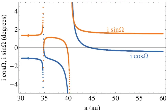
Figure 1 shows how q0 and p0 vary as a function of the test particle’s semi-major axis, using
planetary inclination information from Murray & Dermott (1999). At large semi-major axes (q0,p0)
converges to the invariable plane (the total angular momentum plane of the solar system). But at 35 and 40.3 au the expected forced plane is strongly warped due to secular resonance. These are places where f0, essentially the test particle’s natural frequency, is very similar to one of the secular
frequencies (fi).
Note that the forced plane has a time dependence. Like the inclination vectors of the planets themselves, the forced inclination of a test particle is a vector sum of contributions from the secular inclination eigenmodes, which each rotate in (q,p) space. The test particle also generally has a free inclination that adds another vector to this vector sum. Thus, the (total) inclination of a test particle will oscillate around the forced inclination, which in turn will ultimately oscillate around the invariable plane.
2.2. Survey Simulation
If all Kuiper Belt objects were known, then the symmetry center of all objects in (q, p) space would correspond to the current forcing plane. However, surveys of the Kuiper Belt can only provide an observationally biased subset of the population, introducing effects which skew the derived plane
(Brown & Pan 2004; Volk et al. 2017). Any given survey only points in certain directions, only
Plane of the Kuiper Belt ••••••••••••••••••••••••••••••••••••••••••••••••••••••••••••••••••••••••••••••••••••••••••••••••••••••••••••••••••••••••••••••••••••••••••••••••••••••••••••••••••••••••••••••••••••••••••••••••••••••••••••••••••••••••••••••••••••••••••••••••••••••••••••••••••••••••••••••••••••••••••••••••••••••••••••••••••••••••••••••••••••••••••••••••••••••••••••••••••••••••••••••••••••••••••••••••••••••••••••••••••••••••••••••••••••••••••••••••••••••••• ••••••• • • • • • • • • • • • •• •••• •••••••••••• •••••••••••••••••••••••••••••••••••••••••••••••••••••••••••••••••••••••••••••••••••••••••••••••••••••••••••••••••••••••••••••••••••••••••••••••••••••••••••••••••••••••••••••••••••••••••••••••••••••••••••••••••••••••••••••••••••••••••••••••••••••••••••••••••••••••••••••••••••••••••• ••••••••••••••••••••••••••••••••••••••••••••••••••••••••••••••••••••••••••••••••••••••••••••••••••••••••••••••••••••••••••••• ••••••••••••••••••••••••••••••••••••••••••••• ••••••••••••••••••••••• ••••••••••••• ••••••••• ••• ••• ••••• •• •••••• •••• ••••• ••••••••••••• ••••••••••••••••••••• ••••••••••••••••••••••••••••••••••••••••• ••••••••••••••••••••••••••••••••••••••••••••••••••••••••••••••••••••••••••••••••••••••••••••••••••••••••••••••• •••••••••••••••••••••••••••••••••••••••••••••••••••••••••••••••••••••••••••••••••••••••••••••••••••••••••••••••••••••••••••••••••••••••••••••••••••••••••••••••••••••••••••••••••••••••••••••••••••••••••••••••••••••••••••••••••••••••••••••••••••••••••••••••••••••••••••••••••••••••••••••••••••••••••••••••••••••••••••••••••••••••••••••••••••••••••••••••••••••••••••••••••••••••••••••••••••••••••••••••••••••••••••••••••••••••••••••••••••••••••••••••••••••••••••••••••••••••••••••••••••••••••••••••••••••••••••••••••••••••••••••••••••••••••••••••••••••••••••••••••••••••••••••••••••••••••••••••••••••••••••••••••••••••••••••••••••••••••••••••••••••••••••••••••••••••••••••••••••••••••••••••••••••••••••••••••••••••••••••••••••••••••••••••••••••••••••••••••••••••••••••••••••••••••••••••••••••••••••••••••••••••••••••••••••••••••••••••••••••••••••••••••••••••••••••••••••••••••••••••••••••••••••••••••••••••••••••••••••••••••••••••••••••••••••••••••••••••••••••••••••••••••••••••••••••••••••••••••••••••••••••••••••••••••••••••••••••••••••••••••••••••••••••••••••••••••••••••••••••••••••••••••••••••••••••••••••••••••••••••••••••••••••••••••••••••••••••••••••••••••••••••••••••••••••••••••••••••••••••••••••••••••••••••••••••••••••••••••••••••••••••••••••••••••••••••••••••••••••••••••••••••••••••••••••••••••••••••••••••••••••••••••••••••••••••••••••••••••••••••••••••••••••••••••••••••••••••••••••••••••••••••••••••••••••••••••••••••••••••••••••••••••••••••••••••••••••••••••••••••••••••••••••••••••••••••••••••••••••••••••••••••••••••••••••••••••••••••••••••••••••••••••••••••••••••••••••••••••••••••••••••••••••••••••••••••••••••••••••••••••••••••••••••••••••••••••••••••••••••••••••••••••••••••••••••••••••• ••••••••••••••••••••••••••••••••••••••••••••••••••••••••••••••••••••••••••••••••••••••••••••••••••••••••••••••••••••••••••••••••••••••••••••••••••••••••••••••••••••••••••••••••••••••••••••••••••••••••••••••••••••••••••••••••••••••••••••••••••••••••••••••••••••••••••••••••••••••••••••••••••••••••••••••••••••••••••••••••••••••••••••••••••••••••••••••••••••••••••••••••••••••••••••••••••••••••••••••••••••••••••••••••••••••••••••••••••••••• ••••••• ••• • • • • • • • • • • •••• ••••••••••• ••••••••••••••••••••••••••••••••••••••••••••••••••••••••••••••••••••••••••••••••••••••••••••••••••••••••••••••••••••••••••••••••••••••••••••••••••••••••••••••••••••••••••••••••••••••••••••••••••••••••••••••••••••••••••••••••••••••••••••••••••••••••••••••••••••••••••••••••••••••••••••••••••••••••••••••••••••••••••••••••••••••••••••••••••••••••••••••••••••••••••••••••••••••••••••••••••••••••••••••••••••••••••••••••••••••••••••••••••• •••••••••••••••••••••••••••••••••••••••••••••••••••••••• ••••••••••••••••••• ••••••••• ••• ••• •• •• • • • • • • • • • • ••• •••• •••••••••••• •••••••••• •••••••••••••••••••••••••••••••••••••••••••••••• ••••••••••••••••••••••••••••••••••••••••••••••••••••••••••••••••••••••••••••••••••••••••••••••••••••••••••••••••••••••••••••••••••••••••••••••••••••••••••••••••••••••••••••••••••••••••••••••••••••••••••••••••••••••••••••••••••••••••••••••••••••••••••••••••••••••••••••••••••••••••••••••••••••••••••••••••••••••••••••••••••••••••••••••••••••••••••••••••••••••••••••••••••••••••••••••••••••••••••••••••••••••••••••••••••••••••••••••••••••••••••••••••••••••••••••••••••••••••••••••••••••••••••••••••••••••••••••••••••••••••••••••••••••••••••••••••••••••••••••••••••••••••••••••••••••••••••••••••••••••••••••••••••••••••••••••••••••••••••••••••••••••••••••••••••••••••••••••••••••••••••••••••••••••••••••••••••••••••••••••••••••••••••••••••••••••••••••••••••••••••••• •••••••••••••••••••••••••••••••••••••••••••••••••••••••••••••••••••••••••••••••••••••••••••••••••••••••••••••••••••••••••••••••••••••••••••••••••••••••••••••••••••••••••••••••••••••••••••••••••••••••••••••••••••••••••••••••••••••••••••••••••••••••••••••••••••••••••••••••••••••••••••••••••••••••••••••••••••••••••••••••••••••••••••••••••••••••••••••••••••••••••••••••••••••••••••••••••••••••••••••••••••••••••••••••••••••••••••••••••••••••••••••••••••••••••••••••••••••••••••••••••••••••••••••••••••••••••••••••••••••••••••••••••••••••••••••••••••••••••••••••••••••••••••••••••••••••••••••••••••••••••••••••••••••••••••••••••••••••••••••••••••••••••••••••••••••••••••••••••••••••••••••••••••••••••••••••••••••••••••••••••••••••••••••••••••••••••••••••••••••••••••••••••••••••••••••••••••••••••••••••••••••••••••••••••••••••••••••••••••••••••••••••••••••••••••••••••••••••••••••••••••••••••••••••••••••••••••••••••••••••••••••••••••••••••••••••••••••••••••••••••••••••••••••••••••••••••••••••••••••••••••••••••••••••••••••••••••••••••••••••••••••••••••••••••••••••••••••••••••••••••••••
30
35
40
45
50
55
60
-4
-2
0
2
4
a
HauL
i
cos
W
,
i
sin
W
Hdegrees
L
i cos
W
i sin
W
Figure 1. The expected forced i0cos Ω0 (blue) and i0sin Ω0 (orange) of a test particle as a function of its
semi-major axis, given the 8 known planets (from Eqn 4). The features evident at a ≈34.8 and 40.5 au are caused bysecular resonances with the planetary system. The large-a limit is the invariable plane, with (iIcos ΩI, iIsin ΩI) and iI= 1.578o and ΩI = 107.58o in J2000 ecliptic coordinates.
and then any given object might not be recovered by subsequent observations (i.e. be ‘lost’). Most of the detections available in the compilation of TNOs in the IAU Minor Planet Center cannot be tied to a survey for which detection efficiency as a function of orbit and absolute magnitude could be calculated. However, ‘characterized’ surveys (Petit et al. 2011; Jones et al. 2006) provide the information which allows one to compute if an object with given orbit and absolute magnitude would be visible in a survey (or at least a probability of detection as a function of the resulting apparent magnitude on an observation date where the object is in the field). Use of a ‘survey simulator’ (Petit
et al. 2011; Lawler et al. 2018) then enables direct comparison of a model trans-Neptunian belt to
the real observed trans-Neptunian objects.
Our primary characterized survey is OSSOS, whose 838 characterized detections are by far the largest characterized set available for study (Bannister et al. 2018). This survey provides a huge number of non-resonant TNOs, with orbits measured at higher precision than most in the MPC, and completely dominates the statistics for our studies of the main classical Kuiper Belt. We consider only the single-color r band survey of OSSOS for the main trans-Neptunian belt as including other characterized surveys adds complications (e.g. making assumptions about TNO colors), while not significantly affecting the results.
Because we know the sky coverage of each group of survey pointings along with the probability of detection as a function of TNO magnitude and rate of motion, we can evaluate the probability of detecting any given TNO. Repeating this evaluation over very large number of simulated objects
drawn from a specified underlying distribution builds up the population of ‘simulated detections’. These simulated detections can then be compared to the real OSSOS detections, to ascertain whether the proposed trans-Neptunian belt is consistent with the real trans-Neptunian belt.
Beyond a=50 au, however, the wide distribution of inclinations(Gulbis et al. 2010;Petit et al. 2017)
and lower overall detection frequency (due to their more distant orbits) results in in fewer detected objects in the invariable-plane-focused sky coverage of OSSOS, and better statistics are required. We supplement OSSOS detections in a > 50 au with those of three smaller characterized surveys:
• The Canada-France Ecliptic Plane survey (CFEPS), which is a wider but shallower survey mostly in g band near the ecliptic (Petit et al. 2011);
• The CFEPS High Latitude extension (HiLat, Petit et al. 2017), which explored the sky away from the ecliptic, to strongly constrain the form of the tail of the inclination distribution; • The study ofAlexandersen et al.(2016), which targetedthe near-ecliptic sky ahead of Neptune
to maximize detections of leading Neptune trojans and Plutinos.
All of these works provide the information needed to do the modelling described herein. The earlier survey of Schwamb et al.(2010) would provide a small number of additional a > 50 au non-resonant TNOs, but as it has a comparatively low-precision detection efficiency function, we elected not to incorporate it.
The orbital distribution models we use here can remain simple, as our testing showed that the results were largely insensitive to assumptions about the orbital distributions, outside the parameter space of orbital inclination and longitude of ascending node. Because we are trying to constrain the distribution of orbital planes (or, equivalently, angular momentum unit vectors), major changes in semi-major axis distribution, orbital eccentricity and argument of perihelion made only tiny differ-ences to the simulated distribution of detected nodes and orbital inclinations. We always assumed that the mean anomalies were uniformly distributed, and that the nodal longitudes were uniformly distributed in angle around the hypothesized forced plane. Because it continues to provide adequate fits to the observational data, we use the common parameterization of the inclination distribution (Brown 2001;Kavelaars et al. 2009;Petit et al. 2011;Gulbis et al. 2010;Petit et al. 2017) which has the probability density function
f (i) = sin i √1
2πσ e
−i2/(2σ2)
, (5)
with the width σ thus being the only parameter. Figure 2 shows example inclination distributions for different widths. While this formulation may not be reality, the data as yet provide no compelling reason to move to something else.
We have confirmed that assumptions about the absolute magnitude (Hr) distribution make little
difference to our results. This is not surprising, because the largest physical effect for in- or near-plane surveys like OSSOS is simply whether the ascending node is in the direction of the survey or 180 degrees away (for objects at their descending node in the survey). For most of our studies we used a single exponential distribution with dN ∝ 10αH with α=0.8, but we also tested in several cases that
our conclusions about the forced plane did not change if we used the best fit ‘knee’ distribution from
Plane of the Kuiper Belt
0 2 4 6 8
inclinationH°L
relative
number
Figure 2. Examples of inclination distributions generated by the survey simulator, of the functional form sin i times a Gaussian (Eqn 5). The black, grey, and light grey distributions have widths of 1.5, 2.0, 2.5 degrees, respectively.
In this paper we compare the real detections from the survey (or surveys) being simulated to the population of simulated detections via a bootstrappedKolmogorov-Smirnov (KS) statistic. (We also computed the Anderson-Darling (AD) statistics, and got similar results, so we do not present this less-familiar statistic). For every survey simulation we generate 15000 simulated detections. Of these we randomly pick out a sample equal to the number of real detections, and compare the KS statistic of the real TNOs to the KS statistic of the simulated-detected subsample for each of the q, p, i, and Ω cumulative distributions. The distribution of this boot-strapped statistic provides 95% and 99% confidence ranges with which the rejectability of the real sample can then be judged. Because q and p are defined on the interval [−1, 1] and the signal is ‘in the middle’ of this range, the KS test is well adapted to these variables. Because both the q and p distributions need to be non rejectable, we construct a single ‘joint’ statistic for any given comparison by taking the most rejectable of these two 1-D distributions. (This is because a distribution which is fine in one variable but terrible in the other should be rejected by the joint test, and we found that the ‘worst of the two’ approach gave the most sensible answers when we examined the distributions of the dynamical variables). We thus extract random subsamples 3000 times and compute the joint q, p statistic of that sample relative to the entire simulated sample, in order to create the bootstrap. If the joint KS value of the real sample (relative to the entire simulated detection sample from that assumed model) is beyond 95%/99% of the bootstrap KS values, we reject that model at 95% or 99% significance, respectively.
In principle, the q, p distributions should contain the same information as the i, Ω distributions. However, the KS test is best at discerning how different the centers of the compared distributions are. Thus, expressing the orbit planes in terms of q, p versus i, Ω can yield slightly different results for the bootstrapped KS statistic. In particular, q, p are good at locating what q, p are allowed as forced planes, while i, Ω provides information on whether the distribution of TNOs in q, p space is too narrowly or widely concentrated. For example, this difference appears in Figure3 versus Figure 4.
3. THE MAIN BELT
In this section we concentrate on the ‘main belt’ between the 3:2 and 2:1 resonances with Neptune, seeking to determine if the true forced plane is consistent with the expected forced plane from secular theory and to determine what the width of the inclination distribution is for the dynamically ‘cold’ and ‘hot’ populations.
Because the forced plane location is semi-major axis dependent (Fig. 1) the comparison of the real sample to the theoretical prediction is most easily done after binning the objects by orbital a. In previous studies, workers have chosen for their semimajor axis bins either small ranges around important values of a to illustrate the secular effect (Chiang & Choi 2008), essentially no bins at all
(Brown & Pan 2004), or a combination of divisions based on the secular structure and round numbers
(Volk et al. 2017). Because the data set is now larger, we are able to study the variation of theplane
with a and have elected to use dynamical structures observed in the main-belt’s semi-major axis distribution to set the semi-major axis bins, and we also separate the dynamically ‘hot’ and ‘cold’ populations (how these populations are separated is discussed in detail below). Because the values of a and e have only a small effect on detectability on either side of any bin boundary, the divisions we chose make no real influence on the conclusions.
Several previous studies have investigated what the mean plane and inclination widths of the main belt’s subpopulations. Brown (2001) showed that the inclination distribution could be reasonably represented by two dominant components, each of Eq. 5’s form, (around the ecliptic in that paper) with a ‘cold’ component of width 2.2◦ and a hot component of width 18◦. Brown & Pan(2004) derive that the inclination width of the ‘classical belt’ (with no precise orbital element range supplied) is 1.3◦ and 12.0◦ for the cold and hot components. They referred all objects’ inclinations to a ‘Kuiper Belt plane’ that they calculated and after debiasing the objects with respect to that plane using the
Brown (2001) method. Elliot et al. (2005) do not derive inclination widths, but derive mean planes
for a variety of subsets of the TNO population detected in the Deep Ecliptic Survey (DES), with wide semi-major axis bins which are centered in the range ∼40–45 au. Their results disagree with the ‘Kuiper belt plane’ calculated by Brown & Pan (2004) at the roughly 2 sigma level. (Adams et al.
(2014) do derive inclination widths for the DES.) Gulbis et al. (2010) find a cold width of 2.0±0.5◦ upon further analysis of the DES data set. Volk et al. (2017) showed how the mean plane in the main-belt region appears to follow the expected secular solution, pointing out that theBrown & Pan
(2004) method requires an assumption on the widths to estimate uncertainties in the derived mean plane. In this context, we seek to provide an independent analysis of the main-belt region’s forced
plane using the almost entirely independent OSSOS sample, while using a method that is directly sensitive to the inclination widths.
For the semi-major axis bins, we have elected to use the the knowledge of the cold main-belt’s substructure discovered in CFEPS (Petit et al. 2011) and confirmed by OSSOS (Bannister et al. 2016). Specifically, between the 3:2 and 2:1 resonances the cold belt has discernible (a, e) substructure with a concentrated ‘kernel’ from 43.8 to 44.4 au superposed on a wider ‘stirred’ population from 42.4 to 47.0 au (see below how this is used in a study of how the forcedplanemoves with semimajor axis). Thus, for the ‘cold’ component we split the region into three bins: 42.4 –43.8 au, 43.8 – 44.4 au, and 44.4 – 47 au. For the ‘hot’ cosmogonic component of the main belt, we lump all objects into one bin spanning 42.4 – 47.0 au. Here the much larger inclination width means that the expected change in the forced plane position over the classical belt’s semi-major axis range is only a small fraction of the inclination width.
3.1. The Cold Population
Because in the main classical Kuiper Belt both the cold and hot populations coexist as two overlap-ping components in parameter space, to study the cold population we first need to isolate it somehow in the observed sample. At low inclinations the cold component will dominate and at high inclinations
Plane of the Kuiper Belt
the hot population will dominate, but no simple i cut can perfectly separate the populations. Adding compositional information (which can be revealed through observations of a TNO in multiple color filters) can aid in distinguishing unique components (e.g. Pike et al. 2017), but only the brightest ∼ 10% of OSSOS discoveries yet have additional colour observations (Schwamb et al. 2018). Here we segregate the ‘cold component’ by considering only objects within 4o of each proposed forced plane. This is equivalent to limiting ourselves to objects with free inclinations < 4o relative to each proposed
forced plane. With such a cut, we will get very few interlopers from a hot population. We also tried a cut of 5o and found substantially similar results. Our choice of cut is motivated by Dawson &
Murray-Clay (2012) Figure 2, showing contamination of the cold population by the hot population
as a function of inclination cut.
The location of the forced plane moves over this range of semimajor axes, so we split the sample into a number of semi-major axis bins. As discussed above, we have chosen to split the main belt into three semimajor axis bins: 42.4 – 43.8 au, 43.8 – 44.4 au, and 44.4 – 47 au. Because we cut in inclination relative to each hypothetical forced plane, the number of real objects we compare to each survey simulated sample will depend on forced plane as well as the semimajor axis bin. Assuming the forced plane is that expected from secular theory, the aforementioned bins have 107, 82, and 67 real cold (if ree < 4o) objects.
3.1.1. The Forced Plane
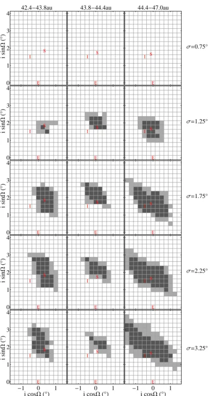
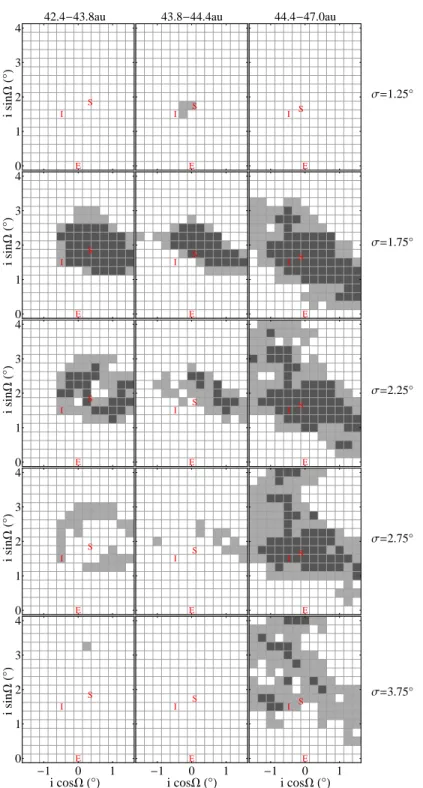
From Figures 3 and 4, we can see that most of the forced planes we tested are rejectable (white boxes in these figures are rejected at 99% confidence). Only a confined region around the expected secularly forced plane is steadily consistent with the observed OSSOS sample. The only case where the expected secularly forced plane becomes rejectable is if the width of the inclination distribution (σ) is too narrow or too wide, as tested by the i,Ω distribution (Figure4). (Exactly what inclination widths are allowed depends on the semimajor axis bin, details of which are discussed in the next section.)
In the 42.4 – 43.8 au and 43.8 – 44.4 au semi-major axis ranges,the allowed (non-rejectable) values for the forced plane cluster in q, p space around the expected q0, p0 from secular theory, while both the ecliptic plane and invariable plane are rejected for all inclination widths. At these semimajor axes, the difference between the expected forced plane and the invariable plane is due to the influence of the ν18 secular resonance. In the 44.4 – 47 au range the forced plane (and the inclination width, σ) is less constrained due to fewer if ree < 4 objects. Here, the invariable plane is not rejectable, but
in this region the expected secularly forced plane is not so different from the invariable plane since as semi-major axis increases the secularly forced plane approaches the invariable plane (Figure 1).
Overall, we agree with Volk et al. (2017) that the main Kuiper Belt nicely follows the expected secularly forced plane. Volk et al. (2017) note that in their two (overlapping) outermost bins in this region they see a weak discrepancy from the expected forced plane. While we do not see such a discrepancy, disagreements of this weak statistical significance are reasonable when comparing results from two independent data sets.
3.1.2. The Width of the Cold Inclination Distribution
Previous understanding of the inclination distribution was achieved by finding widths of the dis-tribution that were non-rejectable (Petit et al. 2011; Gulbis et al. 2010). There were simply too few
42.4-43.8au 43.8-44.4au 44.4-47.0au i sin W H°L -1 0 1 4 3 2 1 0 -1 0 1 4 3 2 1 0 E I S -1 0 1 4 3 2 1 0 -1 0 1 4 3 2 1 0 E I S -1 0 1 4 3 2 1 0 -1 0 1 4 3 2 1 0 E I S Σ=0.75° i sin W H°L -1 0 1 4 3 2 1 0 -1 0 1 4 3 2 1 0 E I S -1 0 1 4 3 2 1 0 -1 0 1 4 3 2 1 0 E I S -1 0 1 4 3 2 1 0 -1 0 1 4 3 2 1 0 E I S Σ=1.25° i sin W H°L -1 0 1 4 3 2 1 0 -1 0 1 4 3 2 1 0 E I S -1 0 1 4 3 2 1 0 -1 0 1 4 3 2 1 0 E I S -1 0 1 4 3 2 1 0 -1 0 1 4 3 2 1 0 E I S Σ=1.75° i sin W H°L -1 0 1 4 3 2 1 0 -1 0 1 4 3 2 1 0 E I S -1 0 1 4 3 2 1 0 -1 0 1 4 3 2 1 0 E I S -1 0 1 4 3 2 1 0 -1 0 1 4 3 2 1 0 E I S Σ=2.25° i sin W H°L -1 0 1 4 3 2 1 0 -1 0 1 4 3 2 1 0 E I S -1 0 1 4 3 2 1 0 -1 0 1 4 3 2 1 0 E I S -1 0 1 4 3 2 1 0 -1 0 1 4 3 2 1 0 E I S Σ=3.25°
i cosWH°L i cosWH°L i cosWH°L
Figure 3. Joint bootstrapped KS statistic for the q, p distributions, for different semi-major axis bins (columns), width of the inclination distribution (rows), and forced planes (i cos Ω,i sin Ω). Any bootstrapped statistic above 0.05 displays as dark grey, bootstrapped statistics between 0.05 and 0.01 are light grey (i.e. 95% and 99% confidence limits, respectively). The red E, I, and S denote the ecliptic, invariable, and expected secular forced plane, respectively. The displayed S is the expected forced plane for a TNO with semimajor axis at the mid point of each semimajor axis bin. Note that because of dependence on TNO semimajor axis (Eqn4) the location of S is different in the different semimajor axis ranges, and also within each semimajor axis range.
Plane of the Kuiper Belt 42.4-43.8au 43.8-44.4au 44.4-47.0au
i sin W H°L -1 0 1 4 3 2 1 0 -1 0 1 4 3 2 1 0 E I S -1 0 1 4 3 2 1 0 -1 0 1 4 3 2 1 0 E I S -1 0 1 4 3 2 1 0 -1 0 1 4 3 2 1 0 E I S Σ=1.25° i sin W H°L -1 0 1 4 3 2 1 0 -1 0 1 4 3 2 1 0 E I S -1 0 1 4 3 2 1 0 -1 0 1 4 3 2 1 0 E I S -1 0 1 4 3 2 1 0 -1 0 1 4 3 2 1 0 E I S Σ=1.75° i sin W H°L -1 0 1 4 3 2 1 0 -1 0 1 4 3 2 1 0 E I S -1 0 1 4 3 2 1 0 -1 0 1 4 3 2 1 0 E I S -1 0 1 4 3 2 1 0 -1 0 1 4 3 2 1 0 E I S Σ=2.25° i sin W H°L -1 0 1 4 3 2 1 0 -1 0 1 4 3 2 1 0 E I S -1 0 1 4 3 2 1 0 -1 0 1 4 3 2 1 0 E I S -1 0 1 4 3 2 1 0 -1 0 1 4 3 2 1 0 E I S Σ=2.75° i sin W H°L -1 0 1 4 3 2 1 0 -1 0 1 4 3 2 1 0 E I S -1 0 1 4 3 2 1 0 -1 0 1 4 3 2 1 0 E I S -1 0 1 4 3 2 1 0 -1 0 1 4 3 2 1 0 E I S Σ=3.75°
i cosWH°L i cosWH°L i cosWH°L
Figure 4. Joint bootstrapped KS statistic for the i, Ω distributions, for different semi-major axis bins (columns), width of the inclination distribution (rows), and forced planes (i cos Ω,i sin Ω), c.f. Figure 3. Note that the values of σ shown (rows) are different in this figure versus Figure 3. Not obvious from the diagram is that the inclination distribution is much more sensitive than the node (Ω) distribution. That is, the boundary between rejected and not-rejected is usually caused by the i distribution being rejectable or non-rejectable, the Ω distribution is more permissive (see the text in Section3.1.2).
1.5 2.0 2.5 3.0 0 1 2 3 4 5 ΣHdegreesL reduced Χ 2
Figure 5. Reduced χ2 of the simulated-observed free inclination distribution of the cold component of the main beltcompared to the real-observed free inclination distribution vs width of the inclination distribution (σ) for dotted: 42.4 to 43.8 au, dashed: 43.8 to 44.4, solid: 44.4 to 47.0 au. The minimum χ2 is for σ of 1.5 to 2.0 degrees, and thus inclination distributions of sin(i) times a Gaussian (uniformly distribution around theforced planepredicted by the secular dynamics from the 4 giant planets) provide completely acceptable fits to the detections.
objects from a characterized sample to differentiate among non-rejectable widths. However, OSSOS has now produced a large enough characterized sample to determine the ‘best fit’inclination width. From Figure 4, which shows which forced planes are allowed based on the i, Ω distribution, it is clear that the allowed forced planes vary with the width of the inclination distribution,(σ). The q, p distribution (Figure 3) is not so sensitive to the width of the inclination distribution (as the KS test is most sensitive to the center of a distribution and somewhat less sensitive to that distribution’s shape), and allows a greater range of σ. It is the i, Ω distribution which is most sensitive to whether the width of the inclination distribution istoo narrow or too wide. For example, for a = 42.4-43.8 and 43.8-44.4 au, both inclination widths of 1.25o and 2.25ohave q, p distributionsthat allowforced planes near the expected forced plane, but the i, Ω distribution fails. Specifically, it is the i distribution that determines if a given forced plane is rejected or not. For all of these survey simulations, the Ω distribution is only rejectable if the i distribution is also rejectable. This permissiveness of the Ω distribution is a consequence of the fairly flat shape of this distribution over a wide range of proposed forced planes. This means the Ω cumulative distribution doesn’t change too much and the KS test yields a non-rejectable value.
Given that the ‘expected’ (computed from the four giant planets) forced plane is generally non-rejectable, we now consider what width of the inclination distribution works best assuming that the
expected forced plane is the true forced plane. Figure 5 shows a χ2 test of how well the survey
simulated free inclination distribution matches the observed inclination distribution for different inclination widths (σ in Eqn 5). As done earlier, we only consider TNOs with if ree < 4o in this fit.
From this figure it is apparent that the cold population is best fit by an inclination width near 1.75o. The 43.8 to 44.4 au semi-major axis bin, where the CFEPS L7 kernel (Petit et al. 2011) is located, prefers a slightly lower inclination width but all three bins are satisfactorily represented by σ = 1.75o,
Plane of the Kuiper Belt
i
sin
W
-10 0 10 -10 0 10E
I
KS
Hi,WL 42.4-47.0au Σ=13°
i cosW
i
sin
W
-10 0 10 -10 0 10E
I
KS
Hq,pL 42.4-47.0au Σ=13°
i cosW
Figure 6. Acceptable forced planes derived from the hot population over the semimajor axis range 42.4– 47.0 au, with i > 9o relative to the proposed forced plane. Left: bootstrapped statistic based on the i and Ω distributions. Right: similarly for the q and p distributions. The hot population of the main Kuiper Belt does not provide any additional constraint on which forced planes are non-rejectable. Note that the scale of these figures is much wider than for Figures3and4. Any bootstrapped statistic above 0.05 displays as dark grey, bootstrapped statistics between 0.05 and 0.01 are light grey. The ecliptic (E) and invariable plane (I) are marked in red. The location of the expected forced plane varies appreciably over this range of semimajor axes so we do not mark it on this figure.
which we thus adopt. Although it is possible that the dynamical kernel is indeed more concentrated, more data would be required to prove this.
A narrow width of the inclination distribution limits how much the cold population has been stirred. For example, imagine that a TNO starts with zero free inclination. If the planetary configuration changes suddenly, the TNO’s forced inclination will also change suddenly. This induces a free inclina-tion equal to the vector-difference between the new and old forced inclinainclina-tions. Batygin et al.(2011) suggests it is possible to keep the inclination excitement to reasonable levels during the late stages of migration by controlling the g8 precession rate (primarily controlled by the locations of Neptune
and Uranus). Regardless of that, in models of hot object emplacement, the narrow width of the cold population is a very strong constraint that the vertical velocity kicks must have been very low.
3.2. The Hot Population
As discussed above, there is both a cold population and a hot population in the mid Kuiper Belt. We isolated the cold population by only considering TNOs within 4o of each proposed forced plane. Similarly, we isolate the hot population by considering only TNOs that are more than 9o from each
proposed forced plane (we also tried cutting at 7o and did not get substantially different results).
Due to the lower number of real detections to compare against, splitting into the three semi-major axis bins used for the cold population yields no constraints on the forced plane. When these bins are amalgamated into one (42.4 to 47 au), the forced plane is constrained, but it is a laxer constraint (see Figure 6). The forced planes allowed using only the hot population are consistent with the results
10 12 14 16 18 20 0 1 2 3 4 5 ΣHdegreesL reduced Χ 2
Figure 7. Reduced χ2 vs width of the inclination distribution (σ) of the hot main belt population for 42.4 to 47.0 au. The poorer quality of fit is likely caused by the assumption of a single forced plane over the entire range; see text for discussion.
from the cold population, but the lax constraint from the hot population means that we do not glean any additional information from the hot population on what forced planes are ultimately allowed versus the constraints we have from the cold population.
Like for the cold classicals, we ran a set of survey simulations using a forced plane equal to the expected forced plane for the middle of the bin (here 44.7 au) with a variety of widths for the inclina-tion distribuinclina-tion (σ in Eqn 5). We then calculate the goodness of fit of the inclination distribution. As done earlier, we consider here only TNOs with if ree > 9o. As can be seen in Figure 7, the best
fit width for the hot population is ∼ 13o, but 14o is nearly as good. That said, the fit quality is
somewhat worse than for the cold classicals. Part of the reason for this less-good fit is because we lumped all the hot classicals from 42.4 to 47 au into one bin, and performed survey simulationswith only one q0,p0 for the forced plane; in reality the expected secular forced plane changes noticeably
over the 42.4 to 47.0 au range used. Alternatively, the relatively poorer fit here may also hint that the inclination distribution for the hot classical population is not well fit by a simple inclination distribution of the form in Eqn5. We however did not explore alternates to Eqn5, as we feel a larger number of hot classical TNOs would be required to clearly differentiate between different shapes of the inclination distribution.
4. THE OUTER KUIPER BELT
The outer Kuiper Belt stretches outwards from the 2:1 resonance with Neptune. In this region, the expected secularly forced plane rapidly asymptotes towards the invariable plane (see Figure1). Figure
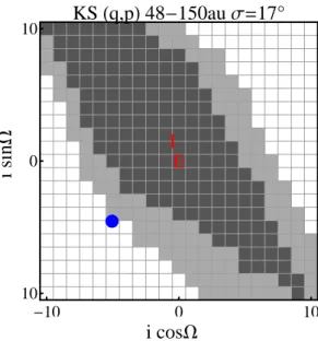
8shows our results for allowed forced planes using TNOs with a = 50 - 80 au (57 objects), and Figure
9 shows our results for 48 - 150 au (83 objects), assuming the width of the inclination distribution (σ in Eq. 5) is 17o (see Figure11 and discussion on the width of the inclination distribution for this
population later in this section for why we chose this value of σ). In both cases, we consider all non-resonant TNOs in the specified (barycentric) semimajor axis bin. The survey simulations here used a single power law of slope 0.8 for the H magnitude distribution, had semimajor axes drawn uniformly over the specified range, and had perihelion distances drawn uniformly from 34.0 to 50 au.
Plane of the Kuiper Belt i sin W -10 0 10 -10 0 10 E I KSHq,pL 50-80au Σ=17° i cosW
Figure 8. Bootstrapped statistics based on the joint q and p distributions for 50-80 au, non-resonant TNOs, with σ = 17o. Any bootstrapped statistic above 0.05 displays as dark grey, bootstrapped statistics between 0.05 and 0.01 are light grey. The blue dot is Volk et al. (2017)’s nominal result for 50-80 au. The observed sample is consistent with the mean plane being the invariable plane, and inconsistent with the nominal result of Volk et al.(2017). See the text for more details.
i sin W -10 0 10 -10 0 10 E I KSHq,pL 48-150au Σ=17° i cosW
Figure 9. Bootstrapped statistics based on the joint q and p distributions for 48-150 au, non-resonant TNOs, with σ = 17o. Any bootstrapped statistic above 0.05 displays as dark grey, bootstrapped statistics between 0.05 and 0.01 are light grey. The blue dot is Volk et al.(2017)’s nominal result for 50-150 au. The observed sample is consistent with the mean plane being the invariable plane, and rejects at 99% confidence the nominal result ofVolk et al. (2017). See the text for more details.
To check if our results depend on the H magnitude distribution we ran sets of survey simulations with the best fit ‘knee’ distribution from Lawler et al. (2018), having a bright slope of 0.9, with a
Figure 10. An example simulation of survey observations of populations for 50-80 au, where the forced plane is the invariable plane and the underlying inclination distribution is has a width of 17o. Small points are simulated observed objects, large circles are real observed objects. Each point is coloured by their observational survey: OSSOS in purple, CFEPS in orange, Alexandersen et al. (2016) in green, and HiLat in blue.
knee at H = 7.7 to a faint slope of 0.4. This choice slightly alters the proportion of objects detected by each of the surveys, but did not have any impact on which forced planes are rejectable.
We also checked if the distribution of perihelion distances would make a difference to our results by running a set of survey simulations with all TNOs’ perihelia equal to 34 au. This extreme case also did not significantly affect the rejectability of various forced planes.
The layout of the entire set of non-rejectable regions in Figures 8 and 9 is a result of an observa-tional sensitivity (or lack thereof) in the different q, p quadrants. Consider Figure 10, which shows q = sin i sin Ω and p = sin i cos Ω of survey simulated detections and real detections. Surveys with pointings at low ecliptic latitudes (like CFEPS and OSSOS) find distant moving objects that are crossing the ecliptic at the observed longitude. A TNO going ‘up’ (from below the ecliptic to above
Plane of the Kuiper Belt 10 12 14 16 18 20 22 24 0 1 2 3 4 5 ΣHdegreesL reduced Χ 2
Figure 11. Reduced χ2 vs width of the inclination distribution (σ) of the outer Kuiper Belt (50-80 au). A 17 degree width around the invariable plane is a good match to the free inclination distribution.
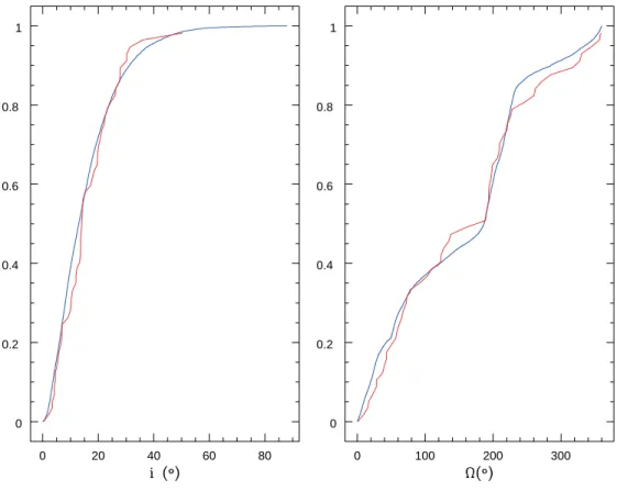
0 20 40 60 80 0 0.2 0.4 0.6 0.8 1 0 100 200 300 0 0.2 0.4 0.6 0.8 1
Figure 12. Cumulative distributions for the inclination and longitude of node for the survey simulation shown in Figure10(50 – 80 au, σ = 17o, invariable as the forced plane). Blue shows the simulated-observed
TNOs, red shows the observed TNOs. This model is not rejectable, with a KS statistic of 0.198 for the joint q, p distributions and of 0.42 for the joint i, Ω distributions.
the ecliptic) will have its ascending node (Ω) at the observed longitude, while a TNO going ‘down’ will have its descending node there. There is no bias favouring TNOs going ‘up’ versus those going ‘down’ (or vice versa), so low latitude surveys populate linear rays on Figure 10that originate from (near) the origin. Surveys with pointings at higher ecliptic latitudes (like the high latitude block of
Alexandersen et al. 2016) also make rays, but these rays are centered off the origin. In such high
latitude surveys, the lowest inclination TNO that is observable has inclination equal to the mini-mum latitude of the pointing. Assuming the survey is north of the ecliptic and orbits are not too non-circular, the lowest-i TNO would have an ascending node 90o behind the observed longitude.
For southern latitudes, the lowest-i TNO would have an ascending node 90o ahead of the observed
longitude. Higher-i TNOs that are observed have their ascending nodes shifted ahead or behind the lowest-i case. The higher a TNO’s inclination, the more its ascending node needs to be shifted from the lowest-i case. Future similar-depth surveys like LSST will provide detections in the upper-left and lower-rightq, pquadrants, which will improve our ability to test forced planes in those directions. The pointings of the OSSOS blocks give us strong sensitivity to ascending nodes in the lower left and upper right q, p quadrants. While CFEPS (Petit et al. 2011), HiLat (Petit et al. 2017), and
Alexandersen et al. (2016) add some coverage in other quadrants, these surveys were either not as
deep or did not cover as much sky. There are approximately as many real objects in the lower left quadrant as in the upper right, and this feature is what makes forced planes in the lower left or upper right of Figures 8and9fail. However, putting the forced plane in the upper left or lower right is consistent with the observed symmetry, making such forced planes non-rejectable by the suite of surveys we have available.
The most important test is to determine if we can reject the invariable plane as the center of the distribution (that is, the expected result if the particle precession is dominated by the four known giant planets). We are unable to do so; the invariable plane is perfectly acceptable as a mean plane given the suite of data sets we use, for both sets of semimajor axis ranges. The reduced chi-squared of the inclination distribution is less than one for the best-match model (Figure 11), and the match of the inclination and nodal longitude distribution is also excellent (Figure 12). We cannot reject the null result: this data set provides no compelling evidence against the invariable plane being the
mean plane beyond Neptune (out to 150 au at least).
Assuming the real forced plane is the invariable plane, Figure 11shows the goodness of fit for the observed inclination distribution versus width σ (Eqn 5). Inclination widths that are too narrow overproduce TNOs with low inclinations, whereas a larger width puts too many TNOs in the high-i tail. We find that the best-fit inclination width is 17o, indicating (albeit weakly) that this distribution
is perhaps wider than for the hot classicals (where the preferred width is 14o; Figure 7). As can be seen in Figure 12, the cumulative distributions of i and Ω for σ of 17o match very well with what
is observed. While the difference in nominal width for the hot classicals and outer non-resonant populations is intriguing, this result is not conclusive proof that the outer Kuiper Belt has a different width than the hot main belt. From Figures 7 and 11, a width of ∼ 15o, for example, is acceptable for both of these populations.
4.1. Constraints on Additional Planets
Volk et al. (2017) found that, using the Brown & Pan (2004) method, the MPC sample of TNOs
indicates that the forced plane for a = 50-80 and 50-150 au is in the lower left q, p quadrant. Their uncertainty in the forced plane was moderately large, though they found it to be inconsistent with the
Plane of the Kuiper Belt
invariable plane at > 95% confidence. Using a largely independent data set and a different analysis method we do not reproduce this rejection of the invariable plane, which we instead find completely acceptable. Our results rule out the nominal forced plane derived for the a=50–80 au MPC sample at > 99% confidence (Figure 8), and most of the lower left q, p quadrant that said nominal forced plane lies in. The 50–150 au sample’s nominal forced plane derived with the Brown & Pan (2004) method is rejected at > 99% confidence by our method applied to the OSSOS sample, but lies near a region that we can reject at only at 95% (Figure 9). There is no compelling evidence from the analysis of the independent data set that a warp in the direction and amplitude found byVolk et al.
(2017) is preferred, although we cannot rule out smaller warps in that direction. Our result is that the expected invariable plane is consistent with the OSSOS data set.
Given the tension between the resultsVolk et al. (2017) and the results presented here, one could ask where the difference between our conclusions could come from. One possibility is that the set of TNOs Volk et al. (2017) were working with, from the Minor Planet Center (MPC) database,
contains systematically incomplete object reports from some surveys. The Brown & Pan (2004) method cannot correctly derive the true forced plane with an incompletely reported data set; it assumes that all TNOs discovered in the survey have had orbits reported. So if some survey(s) did not report all TNOs they discovered to the MPC before Volk et al. (2017) did their analysis,
then Volk et al. (2017) would be working with an incomplete data set. For example, several TNOs
appeared after theVolk et al. (2017) analysis in Minor Planet Electronic Circulars2, but several other TNOs from the same dark run had been reported to the MPC prior to theVolk et al.(2017) analysis. This is interesting especially because these three newly reported TNOs have large inclinations and ascending nodes in the opposite half space of the warp derived by Volk et al. (2017). Incomplete reporting happens for a large variety of reasons, but in this context it means that the set of MPC objects cannot be taken at face value. A final resolution of the tension between these two results for the a=50–80 au sample will require complete data sets, but because we know that the OSSOS data set is calibrated and complete we have reasonable confidence in our model rejection estimates.
Constraining the presence of an additional planet from these results is tricky given the large range of TNO semi-major axes considered here, in particular because the forcing plane varies as a function of the TNO’s semi-major axis (see Section2.1). In the presence of an additional planet in the ∼100 au region, this dependence would be quite dramatic for the TNOs considered here. It is also reasonable to assume that with this additional planet present, the width of the inclination distribution would change as a function of semi-major axis, and is perhaps not at all well described by Eqn 5. For example, if these TNOs are put in place via scattering or resonant interactions with Neptune, they would start symmetrically distributed about Neptune’s mean plane. As time progressed, these TNOs would subsequently precess around the forced plane dictated by their new semimajor axis, which in the presence of an additional planet would not be the invariable plane. Such an emplacement would give the TNO inclination distribution a dependence on TNO semimajor axis. While it is true that our analysis indicates the inclination distribution may be wider for the outer Kuiper Belt than for the hot main classical belt, as would be expected from such a situation with an additional mass, the difference inthese populations’ inclination widthsis not statistically significant enough to be viewed as evidence of an additional planet in the ∼ 100 au region.
2Minor planet electronic circulars 2018-K-118, 2018-K-119, and 2018-K-120 reporting the discoveries/orbital