Effect of in-cylinder liquid fuel films on engine-out unburned hydrocarbon emissions for SI engines

(1)

w

Effect of In-cylinder Liquid Fuel Films on Engine-Out Unburned Hydrocarbon Emissions for SI Engines

by

Vincent S. Costanzo

B.S. Mathematics

B.M.E. Mechanical Engineering Villanova University, 2001 MASSACHUSETTS INSTITUTE OF TECHNOLOGY

MAY 18

2011

LIBRARIES

Effect of In-cylinder Liquid Fuel Films on Engine-Out

Unburned Hydrocarbon Emissions for SI Engines

by

Vincent S. Costanzo

Submitted to the Department of Mechanical Engineering on January 14, 2011 in Partial Fulfillment of the Requirements for the Degree of

Doctor of Philosophy in Mechanical Engineering

ABSTRACT

Nearly all of the hydrocarbon emissions from a modern gasoline-fueled vehicle occur when the engine is first started. One important contributing factor to this is the fact that, during this time,

temperatures throughout the engine are low - below the point at which all of the components of the gasoline can readily vaporize. Consequently, any fuel that enters the combustion chamber in liquid form can escape combustion and subsequently be exhausted as hydrocarbon emissions.

An experimental study was performed in a firing engine in which liquid gasoline films were established at various locations in the combustion chamber and the resulting impact on hydrocarbon emissions was assessed. Unique about this setup was that it combined direct visual observation of the liquid fuel films, measurements of the temperatures these films were subjected to, and the determination from gas analyzers of burned and unburned fuel quantities - all with cycle-level or better resolution.

An increase in the hydrocarbon emissions was observed with liquid gasoline films present in the combustion chamber. This increase depended upon both the location of the film and the temperature of that location, and correlated with estimates of the mass of fuel in the film. The largest impact was observed when the head near the exhaust valve was wetted; the smallest impact was observed when the piston on the intake side of the engine was wetted. In general, as engine temperatures increased the hydrocarbon emissions due to the liquid fuel films decreased. It was also identified when, in the exhaust event, fuel from the films was actually exhausted.

The effect of the location of the liquid fuel film can best be understood in terms of the time before flame arrival at that location, the local flow over the film, and the extent to which the overall flow in the combustion chamber carries fuel from the film to the exhaust valve. The primary effect of wall

temperature is to affect the amount of vaporization from the film: as temperature increases more vaporization occurs before flame arrival, resulting in less fuel that can vaporize post-flame as unburned fuel emissions.

Thesis Supervisor: John Heywood

(4)

(5)

(6)

(7)

LIST OF TABLES

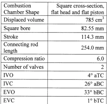
Table 2.1: Geometry and valve information for square piston visualization engine. Valve timings

are lash-adjusted zero-lift values. ... 62

Table 2.2: Flows, concentrations, and mass exchange between combustion chamber and volume beneath the piston . ... 63

Table 2.3: Summary of National Instruments data acquisition hardware... 64

Table 3.1: Summary of operating conditions used (unless otherwise noted)... 105

Table 3.2: Fueling sequence for the quasi-steady liquid deposition experimental scheme... 105

Table 5.1: Summary of experiments used in the study ... 227

Table 5.2: Approximate wetted areas and their distribution on the combustion chamber surfaces for each of the deposition locations ... 228

Table 5.3: Estimated fraction of each injection that sticks to the combustion chamber walls for the first and third depositions at each location. Outliers suspected to be due to accumulated errors are italicized... 228

Table 5.4: Average values of the fraction of each injection that sticks to the combustion chamber walls for each deposition location type. Suspected outliers that were italicized in Table 5.3 were excluded from the averaging... 228

(11)

LIST OF FIGURES

Figure 1.1: Federal unburned hydrocarbon emissions regulations versus initial year of regulation

(For further explanation of the different bases, see note 2 in this chapter.) ... 32

Figure 1.2: Cumulative engine-out and tailpipe-out hydrocarbon emission over the FTP-75 drive

cycle for a six cylinder SI engine, from [5]. ...

32

Figure 1.3: Engine-out hydrocarbon (EOHC) emissions for the first (cold start) and third (hot start) phases of the FTP75 drive cycle, for the same engine as Figure 1.2. (Figure from [8], with m inor m odifications.)... 33

Figure 1.4: Comparison of energy content per unit volume for various fuels suitable for an internal com bustion engine ... 33

Figure 1.5: Schematics of port fuel injection (left) and direct fuel injection (right) ... 34

Figure 2.1: Basic construction of the square piston visualization engine... 65

Figure 2.2: Isometric view (left) and top view (right) schematics of piston and seal bars showing leakage paths, from [2 1]. ... 65

Figure 2.3: Schematic of "volume beneath the piston" ventilator ... 66

Figure 2.4: Front view of ventilator showing reed valves ... 66

Figure 2.5: Installed ventilator: flow paths and gas sampling location ... 67

Figure 2.6: Typical unburned HC concentration in the ventilator and ideal flow rates. 0 degrees is T C -in tak e. ... 6 7 Figure 2.7: Schematic of fuel system, from [19]. ... 68

Figure 2.8: Cross-section of fuel spray for the DI injector used in this study, operating at 44 psi injector rail pressure. Image taken 180 after start of injection, for fired operation with an intake pressure of 0.5 bar and the start of injection at 90' aTC-intake. From [19]. Note that the injector targeting used in [19] was not the same as the targeting used in this study, but the injector and engine are otherw ise the sam e. ... 68

Figure 2.9: DI injector mounted in a targeting plate (removed from the engine)... 69

Figure 2.10: DI injector mounted in a targeting plate (installed in the engine)... 69

Figure 2.11: Pressure data for a typical fired cycle (full view) ... 70

Figure 2.12: Pressure data for a typical fired cycle (detail view showing 0-150 kPa)... 70

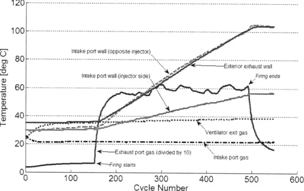
Figure 2.13: Typical gas and non-combustion chamber surface thermocouple measurements. Firing occurs from cycles 150 to 491. Note that the exhaust port gas temperature is divided by 10 ... 7 1 Figure 2.14: Photograph of the surface thermocouples installed in the piston (left) and head and lin er (righ t) ... 7 1 Figure 2.15: Typical combustion chamber surface thermocouple measurements... 72

(12)

Figure 2.17: Tab 2 of the data acquisition VI front panel... 73

Figure 2.18: Tab 3 of the data acquisition VI front panel... 74

Figure 2.19: Block diagram for the data acquisition VI ... 74

Figure 2.20: Front panel of the temperature monitoring VI ... 75

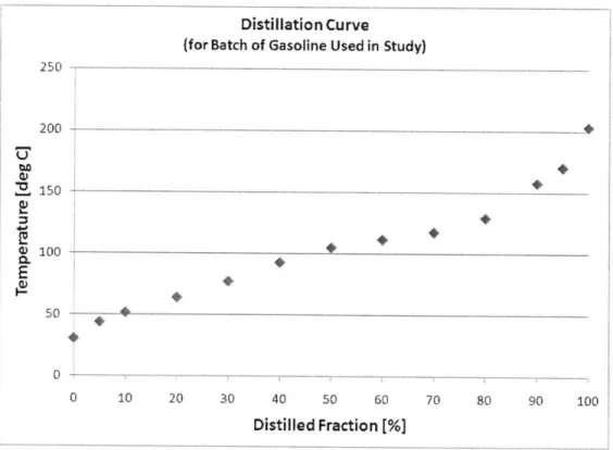
Figure 3.1: Specification sheet for the gasoline used in the study... 106

Figure 3.2: Distillation curve for the gasoline used in the study ... 107

Figure 3.3: Schematic of fuel pathway tracking via carbon tracking ... 107

Figure 3.4: Implementation of fuel pathway tracking via carbon tracking... 108

Figure 3.5: Fuel pathway deduction from the measurement of carbon-containing species... 108

Figure 3.6: Cycle-resolved engine speed for motoring and 150 fired cycles ... 109

Figure 3.7: Intake manifold pressure at intake valve closing versus cycle number and time for a typical experim ent... 109

Figure 3.8: Intake airflow versus cycle number and time for same experiment as Figure 3.7... 110

Figure 3.9: Scatter plot of net imep and exhaust HC emissions versus port injection timing .... 110

Figure 3.10: Net imep and exhaust HC emissions versus batch number (i.e. time in experiment) for the data of Figure 3.9... 111

Figure 3.11: Engine parameters versus spark timing, using only isopentane... 111

Figure 3.12: Spray residence time (tip travel time + injection duration) versus injector pressure differential for various injected fuel quantities... 112

Figure 3.13: Spray vaporization relative to spray vaporization at 30 psi injector pressure differential, for the range of exponents in the characteristic diameter versus injector pressure differential scaling ... 112

Figure 3.14: Weber and Ohnesorge numbers relative to their values at 30 psi injector pressure differential, for the range of exponents in the characteristic diameter versus injector pressure differential scaling ... 113

Figure 3.15: Sample images of sprays that are and are not deflected by the intake flow, for the "head and upper liner" targeting ... 114

Figure 3.16: Momentum flow rate through the intake valve gap ... 115

Figure 3.17: Images 360 after spark for "early" liquid deposition (left) and "late" liquid deposition (right). With "late" deposition, blackbody radiation from soot particles is visible; chemiluminescence from the flame is overpowered by a halogen lamp that is illuminating the combustion chamber. (See text for further explanation.) ... 115

Figure 3.18: Anticipated unburned hydrocarbon emissions versus burned gas relative air-fuel ratio for the conditions of Table 3.2... 116

Figure 3.19: Typical exhaust burned gas relative air-fuel ratio versus cycle number, for stable cycles only. Cycles with liquid deposition are shown in red; those without liquid deposition are b lack ... 1 16

(13)

Figure 3.20: Typical exhaust mass-averaged hydrocarbon emissions versus cycle number, for stable cycles only and the same experiment as Figure 3.19. Cycles with liquid deposition are shown in red; those without liquid deposition are black... 117 Figure 3.21: Exhaust mass-averaged hydrocarbon emissions versus exhaust burned gas relative air-fuel ratio with and without liquid deposition, for the data of Figure 3.19 and Figure 3.20. Cycles with liquid deposition are shown in red; those without liquid deposition are black... 117 Figure 4.1: Typical (a) exhaust hydrocarbon concentration, (b) normalized exhaust flow, and (c) the product of the exhaust hydrocarbon concentration and normalized exhaust flow... 155 Figure 4.2: Expected and actual meter reading mass-averaged exhaust CO & CO2 concentration

b eh av ior... 15 6 Figure 4.3: Effect of fuel composition on the calculation of relative air-fuel ratio from the ratio of CO to CO2 concentrations (assuming fuel-rich combustion). Note that in the notation of

equation 4.8 the horizontal axis is 1/R, not R ... 156 Figure 4.4: Comparison of relative air-fuel ratio as calculated from cycle-resolved CO and CO2 concentration ratio and as reported by the UEGO meter... 157 Figure 4.5: Relative air-fuel ratio - delivered estimate, UEGO reading, and calculated from cycle-resolved CO and CO 2 concentrations... 157

Figure 4.6: Discrepancy between k calculated from exhaust CO and CO2 ratio and as reported by

the U EG O versus the U EG O reading ... 158 Figure 4.7: Total mass of fuel exiting the combustion chamber via the various pathways and the mass of fuel injected each cycle (typical data for 10 stable fueling cycles)... 159 Figure 4.8: Total mass of fuel exiting the combustion chamber via the various pathways and the mass of fuel injected each cycle (typical data for stable fueling cycles in one experiment) (Color coding is identical to Figure 4.7). ... 159 Figure 4.9: Percent of total fuel injected to each of the various pathways, for the same data as F igu re 4 .8 ... 16 0 Figure 4.10: Mass of fuel molecules exiting the combustion chamber for the cycles before,

during, and after a sam ple liquid deposition... 160 Figure 4.11: The "buildup" method for estimating the mass of fuel on the wall ... 161 Figure 4.12: The "decay" method for estimating the mass of fuel on the wall ... 161 Figure 4.13: Schematic of amount of injected liquid fuel exiting the combustion chamber versus cycle num ber, for liquid injection in cycle 1. ... 162 Figure 4.14: Schematic of amount of injected liquid fuel exiting the combustion chamber versus cycle number, for liquid injection in cycles 1 through 8 and using linear superposition of the profile of Figure 4.13. Each color tracks the contribution of a given injection to the total... 162 Figure 4.15: Relative air-fuel ratio versus cycle number for vapor-only fueling. ... 163 Figure 4.16: Mass-averaged exhaust hydrocarbon concentration versus cycle number for vapor-only fueling, for the sam e experim ent as Figure 4.15... 163

(14)

Figure 4.17: Cycle-resolved mass-averaged exhaust hydrocarbon concentration versus cycle-resolved relative air-fuel ratio for vapor-only fueling, for the same data as Figure 4.15 and Figure 4 .16 ... 16 4 Figure 4.18: Actual and predicted (from fit) exhaust unburned hydrocarbon emissions versus

cycle num ber for the data of Figure 4.17... 164

Figure 4.19: Predicted (from fit) versus actual exhaust unburned hydrocarbon emissions for the data of F igure 4 .18... 165

Figure 4.20: Schematic of method 1 for subtracting off the vapor contribution to the exhaust hydrocarbon emissions: crevices are assumed to be at the burned gas composition. The vertical line segment shows the contribution of the liquid fuel film to the emissions under this assum ption for point "2"... 166

Figure 4.21: Schematic of method 2 for subtracting off the vapor contribution to the exhaust hydrocarbon emissions: crevices are assumed to be at the "vapor-only" composition. The vertical line segment shows the contribution of the liquid fuel film to the emissions under this assum ption for point "2"... 166

Figure 5.1: Labeled views of the combustion chamber that are used to subsequently show the wetted footprints for each of the deposition locations... 229

Figure 5.2: Wetted footprint for the "head and upper liner - intake side" deposition... 230

Figure 5.3: Wetted footprint for the "head and upper liner - exhaust side" deposition ... 230

Figure 5.4: Wetted footprint for the "liner - intake side" deposition ... 231

Figure 5.5: Wetted footprint for the "liner - exhaust side" deposition... 231

Figure 5.6: Wetted footprint for the "piston and mid-liner - intake side" deposition... 232

Figure 5.7: Wetted footprint for the "piston and mid-liner - exhaust side" deposition... 232

Figure 5.8: Combustion chamber surface thermocouple readings versus time and batch number (for the schem e of section 3.4)... 233

Figure 5.9: Location of the combustion chamber surface thermocouples. (This figure uses the same images as Figure 5.1, but the thermocouple locations are now highlighted in yellow. In black and white the thermocouple locations are the white spots not present in Figure 5.1). ... 233

Figure 5.10: Representative wall film temperature for each liquid deposition versus time and batch num ber (for the schem e of section 3.4)... 234

Figure 5.11: Increase in hydrocarbon emissions due to liquid fuel films versus time in the experiment for various liquid deposition locations and the same mass of liquid injected. The first and third points for each deposition location occur at an overall relative air-fuel ratio of 0.83 and are shown with a thick outline; the second and fourth points occur at an overall relative air-fuel ratio of 0.87 and are shown with a thin outline... 235

Figure 5.12: Increase in hydrocarbon emissions due to liquid fuel films versus representative wall film temperature for various liquid deposition locations and the same mass of liquid injected. The first and third points for each deposition location occur at an overall relative air-fuel ratio of 0.83 and are shown with a thick outline; the second and fourth points occur at an overall relative air-fuel ratio of 0.87 and are shown with a thin outline... 236

(15)

Figure 5.13: Increase in hydrocarbon emissions due to liquid fuel films versus time in the experiment for "liner - intake" wetting and different initial combustion chamber wall

temperatures. The first and third points for each deposition location occur at an overall relative air-fuel ratio of 0.83 and are shown with a thick outline; the second and fourth points occur at an overall relative air-fuel ratio of 0.87 and are shown with a thin outline... 237 Figure 5.14: Increase in hydrocarbon emissions due to liquid fuel films versus time in the

experiment for "head and upper liner - intake" wetting comparing different initial combustion chamber temperatures, amounts of injected liquid fuel, and identical conditions on a different day. The first and third points for each deposition location occur at "more rich" overall relative air-fuel ratio and are shown with a thick outline; the second and fourth points occur at a "less rich" overall relative air-fuel ratio and are shown with a thin outline. See text section 5.5.2 for further explanation of relative air-fuel ratio differences... 238 Figure 5.15: Estimated mass of liquid fuel on the combustion chamber surfaces during the stable fueling cycles for the liquid depositions of Figure 5.11 and Figure 5.12 versus time in the

experiment. 5.00 mg of liquid fuel was sprayed at the combustion chamber walls each cycle of liquid deposition. The first and third points for each deposition location occur at an overall relative air-fuel ratio of 0.83 and are shown with a thick outline; the second and fourth points occur at an overall relative air-fuel ratio of 0.87 and are shown with a thin outline. ... 239 Figure 5.16: Estimated mass of liquid fuel on the combustion chamber surfaces during the stable fueling cycles for the liquid depositions of Figure 5.11 and Figure 5.12 versus representative wall film temperature. 5.00 mg of liquid fuel was sprayed at the combustion chamber walls each cycle of liquid deposition. The first and third points for each deposition location occur at an overall relative air-fuel ratio of 0.83 and are shown with a thick outline; the second and fourth points occur at an overall relative air-fuel ratio of 0.87 and are shown with a thin outline... 240 Figure 5.17: Schematic of the pathways injected liquid fuel can follow. The width of the arrows indicate typical proportions for the data of this study. For reference, the stable wall film mass was roughly I to 4 times the injected liquid mass for the data of this study. ... 241 Figure 5.18: Increase in hydrocarbon emissions due to liquid fuel films (per cycle) normalized by the mass of fuel on the wall during the stable deposition cycles for each deposition versus

representative wall film temperature. The first and third points for each deposition location occur at an overall relative air-fuel ratio of 0.83 and are shown with a thick outline; the second and fourth points occur at an overall relative air-fuel ratio of 0.87 and are shown with a thin o u tlin e . ... 2 4 2 Figure 5.19: Mass increase in hydrocarbon emissions due to liquid fuel films (per cycle)

normalized by the estimated mass of each injection that sticks to the wall versus representative wall film temperature. The first and third points for each deposition location occur at an overall relative air-fuel ratio of 0.83 and are shown with a thick outline; the second and fourth points occur at an overall relative air-fuel ratio of 0.87 and are shown with a thin outline... 243 Figure 5.20: Exhaust hydrocarbon profile for vaporous only fueling, at various relative air-fuel ratios. Exhaust valve opening and closing are 330 bBC and 1 bTC, respectively. Note that the relative air-fuel ratio difference between the curves is not uniform, but is very nearly 0.03 units o f . ... 2 4 4

(16)

Figure 5.21: Typical normalized exhaust flow rate (the integral of the curve is 1) obtained via the methodology of section 4.2. Exhaust valve opening and closing are 330 bBC and 1 bTC,

respectively, and indicated by the vertical dotted lines. ... 244

Figure 5.22: Comparison of average exhaust hydrocarbon profiles from stable cycles without liquid deposition in the liquid deposition experiments to the corresponding average profile from an experiment in which liquid fuel was never deposited, for the relative air-fuel ratio range 0.93 to 0.96. The dashed vertical lines indicate exhaust valve opening and closing... 245

Figure 5.23: Comparison of average exhaust hydrocarbon profiles from stable cycles without liquid deposition in the liquid deposition experiments to the corresponding average profile from an experiment in which liquid fuel was never deposited, for the relative air-fuel ratio range 0.78 to 0.81. The dashed vertical lines indicate exhaust valve opening and closing... 246

Figure 5.24: Comparison of average exhaust hydrocarbon profiles from stable cycles with liquid deposition to the corresponding average profile with vapor-only fueling, for stable cycles from the 1St and 3rd liquid depositions in each experiment that are in the relative air-fuel ratio range 0.81 to 0.84. The dashed vertical lines indicate exhaust valve opening and closing. Note that, in order to more clearly show the differences that are present, the scale in the "head and upper liner - exhaust" plot is different than the others. ... 247

Figure 5.25: Comparison of average exhaust hydrocarbon profiles from stable cycles with liquid deposition to the corresponding average profile with vapor-only fueling, for stable cycles from the 2"d and 4t liquid depositions in each experiment that are in the relative air-fuel ratio range 0.87 to 0.90. The dashed vertical lines indicate exhaust valve opening and closing. Note that, in order to more clearly show the differences that are present, the scale in the "head and upper liner - exhaust" plot is different than the others. ... ₂₄₈

Figure 5.26: Natural luminosity for three different liquid deposition locations, frames 1-3... 249

Figure 5.29: Natural luminosity for three different liquid depositions, frame 10... 252

Figure 5.30: Lifetime of a 3.80 mg drop of gasoline on a metal surface as a function of the surface tem perature. From [41]... ₂₅₂

Figure 5.31: Schematic of the Liedenfrost effect. From [42]. ... 253

Figure 5.32: Lifetime of a 3.75 mg drop of gasoline on a metal surface as a function of the surface temperature and ambient pressure. From [43]... ₂₅₃

Figure A. 1: Net mass of injected liquid fuel exiting the combustion chamber versus cycle number for varying numbers of consecutive injections. For all profiles the first cycle of liquid deposition is cycle 6. ... ₂₇₁ Figure A.2: Actual and "generated from superposition" clean-out profiles for 2 consecutive injection s. ... _{2 7 1} Figure A.3: Actual and "generated from superposition" clean-out profiles for 4 consecutive injectio n s. ... _{2 72}

(17)

Figure A.4: Actual and "generated from superposition" clean-out profiles for 7 consecutive injection s. ... _{2 72}

(18)

(19)

1. INTRODUCTION

1.1. MOTIVATION AND BACKGROUND

1.1.1. Unburned Hydrocarbon Emissions Regulations

Beginning with the 1968 model year, the U.S. government has regulated the emission of unburned hydrocarbons from motor vehicles. These regulations are complex: the intention of what follows is not to be comprehensive but rather to simply give a sense of these regulations over time and at present. Where helpful, further explanation and clarification is given in the endnotes.

The history of U.S. federal unburned hydrocarbon regulations for passenger cars is plotted in Figure 1.1 from 1972 to the present' (data from [1] and [2]). The horizontal axis is the model year in which the regulation was first imposed; the vertical axis is the allowable

hydrocarbon emissions from a standard test procedure, specified as grams of emissions allowed per vehicle mile driven.2

The vertical axis of the plot is logarithmic, and thus the rough trend in these regulations is an exponential drop in allowable hydrocarbon emissions with time. Effective with the 2007

model year, all passenger vehicles sold in the U.S. must satisfy the 0.01 g/mile standard. The need to reduce engines' hydrocarbon emissions to meet these ever-tighter regulations is the underlying motivation of this research.

To put these numbers into perspective, consider that for gasoline a fuel economy of 30 mpg corresponds to roughly 95 grams of fuel consumed per mile. Thus, even at this "good" fuel economy and thus relatively low fuel consumption rate, for today's emissions standards the amount of fuel that can be emitted unburned (0.01 g/mile) is roughly one ten thousandth of the total fuel that is consumed (95 g/mile).

(20)

Further, the actual physical quantity of unburned fuel that can be emitted during typical driving can also be estimated. The standards of Figure 1.1 are based upon the FTP75 drive cycle, which is meant to be representative of typical urban driving [3]. It contains a cold start phase, a transient phase, and a hot start phase; a weighted average of the emissions from these three phases is compared to the regulation standards.

A rough estimate of the quantity of unburned fuel that can be emitted can be obtained by assuming the emissions on a g/mile basis are identical in the three phases of the test, in which case the different weighting factors do not matter. Since the entire test is 11.04 miles and 1874 seconds [3], with this assumption the 0.01 g/mile standard corresponds to roughly 110 mg of fuel, which is a spherical droplet of gasoline approximately 1/4" in diameter. Alternatively and

perhaps more realistically, if all of the unburned hydrocarbon emissions are assumed to occur in the cold start phase of the FTP75 drive cycle4_{, the corresponding quantity of unburned fuel for}

the 0.01 g/mile standard is 173 mg - which is a droplet of gasoline roughly 5/16" in diameter. These estimated quantities of unburned fuel can be emitted in about a half hour of typical vehicle operation.

The fact that these estimates are such small fractions and quantities of fuel underscores how tight the current emissions regulations are, and furthermore how good the technology is that is able to meet them. It also suggests that focused research into the details of the engine and its processes is required if one is to understand possible means of reducing the unburned

(21)

1.1.2. Typical Engine-Out and Tailpipe-Out Unburned Hydrocarbon Emissions

In reality, nearly all of the unburned hydrocarbon emissions from a modern vehicle occur when the engine is first started. This can be seen in Figure 1.2, which shows on a fractional basis the cumulative engine-out and tailpipe-out unburned hydrocarbon emissions versus elapsed time

in the FTP75 test for a particular vehicle. The engine-out emissions are what exit the engine, prior to any exhaust aftertreatment. The tailpipe-out emissions are what the vehicle ultimately

emits after exhaust aftertreatment; it is the tailpipe-out emissions that are regulated.

Aside: the data in Figure 1.2 is somewhat dated, and the emissions certification and model year of the vehicle are unfortunately not known, but the trend in both the engine-out and tailpipe-out emissions is nevertheless the same in current engines [6] [7], the only notable difference being that the time to reach ~95% of the tailpipe-out emissions occurs much sooner in modern engines - of the order 10 to 15 seconds [7].

On a fractional basis, nearly all of the tailpipe-out emissions occur during the initial phases of operation. The engine-out emissions, however, do not vary as substantially with time.

The reason for this significant difference between the cumulative engine-out and tailpipe-out emissions is due to the effectiveness of modern exhaust aftertreatment systems, primarily the

three-way catalyst. When operational, these systems eliminate nearly all of the emissions exiting the engine - resulting in very low tailpipe-out emissions. During the initial phases of engine operation these systems are not yet operational and/or effective, and thus nearly all tailpipe-out

emissions occur when the engine is first started.

Moreover, during this critical time when the exhaust aftertreatment system is not effective at reducing emissions, the actual emissions exiting the engine are increased as well. This can be seen in Figure 1.3, which compares the engine-out unburned hydrocarbon emissions

(22)

(normalized by the injected fuel mass) for the cold start and hot start phases of the FTP75 test for the same vehicle of Figure 1.2. For the cold start phase (recorded as seconds 0 to 505 in Figure 1.2) the engine starts at ambient temperature. For the hot start phase (recorded as seconds 1369 to 1874 in Figure 1.2), the engine was fully warmed up but shutdown for ten minutes prior to being restarted. Other than the initial temperature of the engine and subsystems, these two phases are identical.

In the initial ten seconds of both starts, the unburned hydrocarbon emissions exiting the engine are many times the level established later - and during this time the exhaust

aftertreatment systems are generally not yet hot enough to be operational, resulting in substantial tailpipe-out unburned hydrocarbon emissions. The rise in the cumulative tailpipe emissions for both of these starts is clearly evident in Figure 1.2 at seconds 0 and 1369. A further effect of engine temperature can be seen in that the cold start engine-out emissions are roughly double the hot start engine-out emissions throughout the first two minutes or so of operation.

Thus, during the early phases of engine operation, commonly referred to as the "start" and "warmup", the emissions leaving the engine are higher and the exhaust aftertreatment systems are not yet fully operational. This results in these phases of engine operation constituting nearly all of the unburned hydrocarbon emissions that the vehicle emits.

1.1.3. Strategies to Reduce Unburned Hydrocarbon Emissions

The above suggests two strategies to reduce the unburned hydrocarbon emissions that exit the tailpipe: (1) reduce the unburned hydrocarbon emissions leaving the engine, especially during the critical time when exhaust aftertreatment is ineffective, and (2) improve the exhaust aftertreatment. In particular, strategies to improve the exhaust aftertreatment include improving

(23)

the three-way catalyst effectiveness and/or getting it operational sooner, encouraging chemical

reactions that eliminate the emissions prior to the catalyst (for example with secondary air

injection or substantial spark retard), or even somehow storing the emissions in the exhaust

system until they can later be processed.

This project focuses on an important aspect of the first strategy, the reduction of the

unburned hydrocarbon emissions that leave the engine, and in particular the contribution to those

emissions that is due to the presence of liquid fuel in the combustion chamber. The reduction of

this "wall wetting" contribution is a key component of the emissions control strategies used to

meet current emissions regulations [9].

1.1.4. Gasoline: a Fundamental Problem and Challenge

Gasoline is an outstanding fuel for personal transportation because it has a very high

energy density per unit volume in the form it is stored "onboard" the vehicle. Figure 1.4

compares the energy density of gasoline to some other fuels suitable for an internal combustion

engine. This energy density can be interpreted as the amount of chemical energy carried onboard

the vehicle in a given volume. Gasoline and diesel fuel have comparable energy content,

whereas ethanol has roughly two-thirds and the gaseous fuels have less than one-third the

chemical energy content of gasoline on a per unit volume basis. This high energy density is one

of the reasons gasoline is such an attractive fuel for light-duty transportation.

Gasoline has such a high energy density precisely because it is a mixture of liquid

hydrocarbons. And in fact, it is engineered to have specific properties that make it an excellent

(24)

at ambient temperatures and pressures, but readily vaporizes at typical "warmed up" engine temperatures so that it can be efficiently burned in the engine.

The fundamental problem, however, is that when the engine is "cold" (when it is started) the temperatures in the engine are not sufficient to vaporize all of the gasoline. That is, the very fact that makes gasoline a great fuel for light-duty transportation - that is stored as a liquid but readily vaporizes at typical engine temperatures - causes a challenge when the engine is not at operating temperatures. Any gasoline that does not vaporize can accumulate as liquid films within the combustion chamber. If fuel in those films escapes combustion, it can then be exhausted as unburned hydrocarbon emissions.

And in fact, it is quite likely in a modern engine that liquid gasoline will be present in the combustion chamber under cold engine conditions. The trend in modern engines is from port fuel injection to direct in-cylinder fuel injection. Figure 1.5 shows a schematic of both injection schemes. With port fuel injection the fuel spray is directed at the back of the intake valve; with direct fuel injection the fuel is sprayed directly into the combustion chamber. In both of these scenarios, any liquid fuel that impinges on a "cold" metal wall is unlikely to vaporize and thus is very likely to accumulate within the combustion chamber on its walls.

It is commonly thought that these liquid fuel films in the combustion chamber play a major role in the disproportionately high engine-out unburned hydrocarbon emissions when the engine is first started. The focus of this work is the examination and assessment of that

(25)

1.2. PROJECT FOCUS

The focus of this project is to assess the impact on unburned hydrocarbon emissions of having liquid fuel films present at various locations within the combustion chamber. A more practical rephrasing of this question is: if it is inevitable that liquid fuel will be present in the combustion chamber during and after a cold start, how does the location of that liquid fuel impact unburned hydrocarbon emissions? And furthermore, what is the effect of the local wall temperature the liquid films are subjected to at each of the locations?

1.3. PREVIOUS WORK

Previous studies have examined the relationship between the presence of liquid fuel in the combustion chamber and unburned hydrocarbon emissions. Takeda et al [10] used a specially designed engine to trap and purge the cylinder and intake port contents at a desired phase of operation. This enabled them to determine, on a cycle-by-cycle basis, the quantity of fuel on the intake port walls, on the combustion chamber walls, burned and then exhausted, and exhausted unburned. They observed a correlation between the mass of fuel wetting the

combustion chamber walls and the unburned hydrocarbon emissions, and attributed this rise to "vaperization [sic] of the fuel remaining on the cylinder wall, during the expansion stroke". Due to the nature of these experiments, they could not identify where within the combustion chamber the liquid fuel had accumulated.

Landsberg et al [11] deposited liquid fuel at the intake valve seat while the valve was open and observed a significant increase in hydrocarbon emissions. Deposition of the liquid fuel in the intake port on the side closest to the exhaust valve had a substantially larger impact

(26)

However, with this technique it is not at all clear where within the combustion chamber the liquid fuel goes and/or accumulates.

Kim et al [12] developed a novel technique using special filter paper that absorbed dyed fuel surrogate to identify where within the combustion chamber liquid fuel accumulated, and further the quantity of fuel that had impinged upon a specific location. Experiments using this filter paper were performed under motored conditions in a visualization engine using various fuel injectors. Separately, in a standard engine operating at similar conditions, exhaust hydrocarbon measurements were made and the trends in the unburned hydrocarbon emissions were

"consistent with the findings using the [filter paper] footprints techniques" - it is unclear precisely what this statement means and the effect is not obvious from the data, but it appears that the inference is that larger quantities of liquid fuel on the wall correlated with increased hydrocarbon emissions.

Cho et al [13] used laser-induced fluorescence in a visualization rig to measure, for various port injector targetings, the thickness of liquid fuel films on the cylinder liner under steady state intake flow conditions meant to be representative of both part load and wide open throttle conditions. The mass of liquid fuel on the liner was estimated by integrating the liquid film thickness. Separately, in a standard engine, steady state emissions measurements were made and they found those targetings that resulted in larger masses of fuel on the liner also had higher unburned hydrocarbon emissions.

Finally, a series of studies examining liquid fuel film behavior in a spark-ignition engine were performed at the University of Texas at Austin; those studies pertinent to exhaust emissions are summarized here. The device used for these studies was a specially designed "injection probe" that consisted of a standard port fuel injector connected to a small (-0.2mm ID) tube that

(27)

was mounted in an offset electrode spark plug (normally used for pressure transducer access). The end of this tube had an orifice - by rotating or changing the tube a stream of liquid fuel could be directed at the desired location in the combustion chamber. The main advantage of this method to deposit liquid fuel in the combustion chamber over the method used in the current study (a narrow cone angle DI injector) is that with this method the impingement angle is more or less the same for all of the deposition locations. The disadvantages of this method are that head wetting is not possible, the wetted-footprint is not well-controlled, and that periodic "dribbling" from the tube onto the piston occurred that could not be avoided.

These studies used a similar fueling strategy as the current study. Namely, in order to look at the effect of liquid fuel films in a firing engine environment, the bulk of the fuel was provided as a vapor (either LPG or propane depending upon the specific set of experiments) and roughly 10-20% of the fuel was delivered as a liquid via the injection probe. All results in these studies were obtained at steady state with specified coolant temperatures, and further all results (with and without liquid deposition) were obtained at the same exhaust gas relative air-fuel ratio. The specific relative air-fuel ratio used was = 1.1 (fuel lean). In all cases, they found an increase in unburned hydrocarbon emissions when liquid fuel films were present in the combustion chamber.

The first study in this University of Texas at Austin series was performed by Stanglmaier et al [14]. Gasoline was deposited on the liner and piston. The main findings were that the emissions increase due to the liquid fuel films was relatively insensitive both to deposition timing in the cycle and coolant temperature. From this they concluded that the liquid film vaporization rates were "slow" compared to the engine cycle time. The location that exhibited the most significant increase in unburned hydrocarbon emissions was wetting the liner directly

(28)

below the exhaust valves; wetting the center of the piston had the second largest impact and wetting the liner directly below the intake valves had the smallest impact5. The emissions level with liquid fuel films present (for an injected liquid quantity of 15% of the overall fueling) was roughly two to three times higher than the unburned hydrocarbon emissions with vapor-only fuel.

Li et al [15] performed a follow-up study that found that the increase in emissions due to the liquid fuel films was roughly linear in the amount of fuel delivered as a liquid. Additionally, injector "shut-off' tests were performed and it was found that the 1/e time constant for the

6 gasoline films was roughly 3 to 5 engine cycles at their test conditions .

Huang et al [16] focused on piston wetting and deposited various single-component hydrocarbons onto the piston. For these experiments the coolant temperature was maintained at 45 'C and the piston temperature was estimated from a cycle simulation to be 150 'C. The fraction of injected liquid that ultimately ended up as unburned hydrocarbon emissions ranged from 5 to 20% based upon their methodology7_{. Interestingly, the largest unburned hydrocarbon}

emissions impact occurred with the most volatile fuel (normal pentane, boiling point = 36 'C). Its impact was roughly double that of the other normal alkanes used in the study that had boiling points up to 196 'C. This apparent discrepancy was explained by the fact that the normal

pentane had transitioned to the film boiling regime, whereas the other fuels had not. And furthermore, the expected film evaporation time for their various fuels correlated very well with their observed trend in the unburned hydrocarbon emissions: longer evaporation times had higher unburned hydrocarbon emissions.

Finally, in a subsequent study Huang et al [17] used a subset of the single-component fuels from [16] and varied the engine speed and load. They found that as speed increased, the

(29)

impact of liquid fuel films on unburned hydrocarbon emissions decreased, which they attributed

to a combination of decreased time per cycle for vaporization to occur, higher wall temperatures at higher speed operation and thus less fuel mass on the wall, and increased oxidation due to

more vigorous mixing in the exhaust port. As load increased, the impact of liquid fuel films on

unburned hydrocarbon emissions also decreased. This was attributed to higher wall

temperatures (and thus faster film vaporization and smaller wall films) and higher in-cylinder

temperatures (and thus a longer period of time for which temperatures are high enough for

post-flame oxidation to occur).

There are a number of shortcomings in these previous studies. First, those that did not involve visualization have no measurement-based information on where the liquid fuel films are located. Those studies involving paired visualization engines and standard engines do not

provide simultaneous emissions and visual information, and more importantly many of the visualization studies were not performed in a firing engine environment.

Further, while it is recognized that temperature plays a very important role, no studies

actually measured the temperatures the fuel films were subjected to. The results were either correlated to steady state coolant temperatures or to wall temperatures estimated from cycle

simulations.

Finally, none of these studies varied the overall relative air-fuel ratio, which provides a means to assess (when near stoichiometric or fuel rich) whether or not fuel vaporized from the liquid films mixes with crevice gases and oxidizes.

This study overcomes these shortcomings: direct visual observation is performed simultaneously with exhaust emissions measurements in a firing engine, special thermocouples

(30)

are used to measure the combustion chamber surface temperatures, and different relative air-fuel ratios are examined to assess the possibility of oxidation differences with the various liquid fuel film locations.

(31)

'Prior to 1972 the test procedures were "different enough from the current procedure that the standards are not comparable" [1]; for this reason the regulations are only shown from 1972 onward. Further, except for 1972, the values in this plot are those of the FTP75 drive cycle, which has been used for these regulations since 1975. The 1972 drive cycle was very similar - it simply did not include the "hot start" phase of the FTP75 [3]. More recently, additional drive cycles are used along with the FTP75 drive cycle to certify vehicles. For the sake of comparing historical values, the FTP75 drive cycle standards are examined here.

2 Prior to 1994 the regulations were on a "total hydrocarbon" basis, while model years 1994 and later use a

"non-methane organic gas" basis. Non-"non-methane organic gases are defined as all compounds containing carbon, excluding methane. Total hydrocarbons are defined as all hydrocarbons, including methane [1]. Note in particular that the non-methane organic gas basis includes compounds containing oxygen and other species, whereas the total

hydrocarbon basis does not include such compounds, but does include methane. For practical purposes, these two bases are comparable and generally thought of as the "allowable unburned fuel amount" since they are unreacted or partially reacted fuel molecules. (The fuel is the only significant source of these species exiting the engine.)

3 For comparison to the regulations standards, the emissions level of the FTP75 test can be expressed as 0.207 EcId start + 0.518 Etansient + 0.275 Ehot st, where the Ei's are the emissions levels in g/mile for the respective phases. (from

[2] §86.144-94 and used with data from [4]). Note that the explanation in [3] results in a slightly different expression for the composite value, namely 0.215 Ecoldart + 0.500 Etransient + 0.285 Ehot str. This appears to be

erroneous as it does not take into consideration the fact that the test phases are slightly different distances in the composite weighting defined in [2], which results in slightly different coefficients.

4 The cold start phase is 3.59 miles (using data from [4]); see endnote 3 for the weighting of the cold start phase.

5 Although the deposition locations between the two studies are not completely comparable, the findings in the present study are similar.

6 Again, although the test conditions were not identical, the findings in this study are consistent with this observation.

7 For this study, these values were lower: roughly 1 to 10% of the injected liquid ultimately was exhausted as unburned hydrocarbon emissions.

8 _{The findings in this study were similar: as wall temperature increased the increase in hydrocarbon emissions due to}

(32)

Federal Unburned Fuel Emissions Standards - Passenger Cars

1970 1975 1980 1985 1990 1995

Initial year of regulation 2000 2005 Sin 1 izeV, is zero2010

Figure 1.1: Federal unburned hydrocarbon emissions regulations versus initial year of regulation (For further explanation of the different bases, see note 2 in this chapter.)

100

Chrysler 3.8 L Engine

500 1000 1500 2000

Time (sec)

Figure 1.2: Cumulative engine-out and tailpipe-out hydrocarbon emission over the FTP-75 drive cycle for a six cylinder SI engine, from [5].

10-1 10 *Tier 0 Tier 1 Bin 10 Bin 6 Bnins 5-7 9 (LEV T1 Bin 4-in 3 (ULEV 11)

Prio to 1994 the regulations are on a THC basis.

Subsequent regulations are on a NMOG basis. in 2 (PZEVISULEVt 04 0

(33)

0.06 0.05 0.04 0.03 0.02 0.01 0 200 50 0 -50

I

/1 Speed

7Cold

start

EOHC-j f .

-Hot start

EOHC--100

300

Time (sec)

Figure 1.3: Engine-out hydrocarbon (EOHC) emissions for the first (cold start) and third (hot start) phases of the FTP75 drive cycle, for the same engine as Figure 1.2. (Figure from [8], with minor modifications.) 112% 100% 40 30 20 10 - 0-gasoline diesel 69% ethanol 29% 14% methane @ 200 hydrogen @ 700 atm atm

Figure 1.4: Comparison of energy content per unit volume for various fuels suitable for an internal combustion engine

fl U) CO E U-CO) C,) E 0 UJ 100 E -o G) C'

(34)

Fuel

(35)

2. SETUP

2.1. ENGINE AND SUBSYSTEMS

2.1.1. Square Piston Visualization Engine

The engine utilized for this study was a special visualization engine with a square

cross-section combustion chamber. It is shown schematically in Figure 2.1. The engine was

constructed by adding a visualization section to a standard single-cylinder engine assembly [18].

The original circular cross-section piston is connected to the square cross-section piston by a

rigid connecting rod that is supported by a crosshead bushing. The original combustion chamber

of the engine is not used and is simply vented to the crankcase of the engine (this is not shown in

Figure 2.1) so that there is no net change in the volume of the lower original combustion

chamber plus crankcase system, and thus there is no work in compressing or expanding gases in

the lower unused combustion chamber.

The upper, square section visualization combustion chamber is used. The

cross-section is square so as to provide undistorted optical access to the combustion chamber, which

would otherwise be distorted with curved windows. One inch thick quartz windows form two

opposing walls of the combustion chamber; the other two walls are made of steel.

The piston is sealed by graphite bars as shown in Figure 2.2. These "seal bars" provide a

means of sealing the engine that does not require the use of lubrication oil, which could foul the

windows and make optical access difficult. The bars are pressed against walls of the combustion

chamber by springs, and overlap in lap joints at the corners of the combustion chamber.

(36)

2.1.2. Advantages and disadvantages of the square piston engine

The main advantage of this engine was that it afforded excellent optical access. In particular, the location of the liquid fuel films could directly be verified, and other phenomena in the engine could be observed both for troubleshooting and to assist in explaining trends in the

quantitative data.

An additional benefit of this engine is that, given its construction, there is a considerable amount of space in the combustion chamber that is easily accessible for the installation of instrumentation and additional hardware. In particular, thermocouples, a pressure transducer, and a fuel injector were mounted in the clearance volume of the combustion chamber for this study.

The main disadvantages in using the square piston visualization engine for this study were that it is not cooled, that it has "nonstandard" geometry, and that it is difficult to seal. Because the engine is not cooled, steady state experiments were not possible. This shortcoming required extra levels of engine control hardware and software, and guided the way the

experiments were conducted.

The geometry of this engine is not "standard". While the compression ratio, combustion chamber shape, and of somewhat lesser importance the valve configuration are all quite different from a modem production engine, they are considered an acceptable tradeoff given the other benefits of the engine. The most important factor is that it is a firing engine environment in which to perform the experiments.

Finally, while sealing the engine was difficult, acceptable sealing quality and

(37)

The engine was initially chosen because of its advantages over a more standard engine

-any disadvantages that it posed were either able to be overcome or deemed to be an acceptable tradeoff given the advantages.

2.1.3. Modifications to the engine for this study

The major modifications made to the engine for this study were the addition of a system of interchangeable wall plates used to target the direct fuel injector, and the addition of special surface thermocouples in the combustion chamber.

The direct injector targeting plates were motivated by the "third window" design of Shelby [19]. The initial design of this system simply adapted Shelby's components. Ultimately, however, these components were redesigned to make them more rigid, to make engine sealing easier and more repeatable, and to make changing of the plates possible without disassembly of any other engine components.

These injector targeting plates are further described in section 2.1.6; the combustion chamber surface thermocouples are described in section 2.2.2.

Additionally, the intake and exhaust systems of the engine were completely redesigned, primarily to obtain more rapid intake pressure stabilization and more accurate intake airflow measurements, and to reduce pressure pulsations in the exhaust to facilitate exhaust gas

sampling.

Finally, extensive repairs were made to the engine. The engine was, essentially,

completely rebuilt during this study. Most of these repairs were to improve engine sealing, and included the repair of cracked and chipped sections of the combustion chamber components, the replacement of bent or otherwise damaged combustion chamber components, and the

(38)

realignment of the entire combustion chamber and piston system. In order to facilitate proper alignment of the components, critical pieces were modified to be pinned in place and custom shims and gage blocks were designed to ensure that accurate spacing of components could be maintained and checked. Because of these modifications and improvements, repeatable engine sealing conditions were realized.

2.1.4. Engine Sealing

The most challenging aspect of operating this engine was sealing the combustion chamber. The combustion chamber is formed by two steel plates, a cast iron head, and two quartz windows. Every joint between these components must be sealed and able to withstand combustion pressures and elevated temperatures. Moreover, there are significant blowby paths present in the seal bar design used for the piston sealing that must also be adequately sealed.

The three locations to be sealed in the combustion chamber were the metal-to-metal interfaces, the quartz-metal interfaces, and the piston seal bars. The metal-to-metal interfaces, where it was possible to add glands, were sealed with ring sections. In addition, and where o-ring sections were not possible, these joints were sealed from within the combustion chamber with Permatex "Motoseal 1 Ultimate Gasket Maker Grey" (Permatex item #29132). After investigating and trying many different sealants, this particular sealant was found to provide an excellent combination of gap-filling, adhesion, temperature resistance (it is rated to 200 'C), and fuel resistance.

The quartz windows were sealed against the metal of the combustion chamber with flat rubber gaskets. The sealing of these windows was, by far, the most challenging aspect of sealing the engine. The surface each window sealed against was created by four separate components

(39)

(the two steel walls, the head, and a "base plate" in the crosshead assembly) - the alignment of these four components was critical. Further, any solution to seal the windows had to be both

long-lasting (since the area of the blowby path could change if the gaskets were replaced) as well

as easily removable (since the windows did in fact have to removed occasionally and moreover

were easily chipped and damaged).

Previous studies (e.g. [20]) using this engine used 1/32" silicone rubber sheeting "glued"

to the quartz windows with silicone RTV as the gasket material. The purpose of the RTV was to

hold the rubber sheet in place for assembly. The author had difficulty in obtaining satisfactory

sealing with this approach. The slightest non-uniformity in the overall thickness of the "rubber

sheet plus RTV" resulted in either inadequate sealing (i.e. an immediate leak or, more

commonly, blowout of the gasketing while operating the engine) or breaking of the window

upon clamping due to localized stresses at the non-uniformity. Attempts to improve this method

as well as the investigation of alternate means of sealing the windows constituted a substantial

effort in the development of the experimental techniques. Ultimately, outstanding window

sealing was obtained by using adhesive-backed 1/32" silicone rubber sheeting (40A durometer, McMaster-Carr part number 8991 -K7 11) - the adhesive backing held the gasket in place for assembly; its thickness apparently was uniform enough so that none of the problems described

above with the RTV were encountered.

The final aspect of the combustion chamber to be sealed was the blowby paths in the

piston seal bar assemblies. The primary blowby path was through the gaps in the lap joints of the seal bars, as shown in Figure 2.2. The approach to sealing these pathways in prior studies was to

fill these gaps with high-temperature silicone RTV. The author had difficulty in replicating this