Long-memory processes in global ozone and temperature variations

(1)

HAL Id: hal-00301337

https://hal.archives-ouvertes.fr/hal-00301337

Submitted on 30 May 2006

HAL is a multi-disciplinary open access

archive for the deposit and dissemination of sci-entific research documents, whether they are pub-lished or not. The documents may come from teaching and research institutions in France or abroad, or from public or private research centers.

L’archive ouverte pluridisciplinaire HAL, est destinée au dépôt et à la diffusion de documents scientifiques de niveau recherche, publiés ou non, émanant des établissements d’enseignement et de recherche français ou étrangers, des laboratoires publics ou privés.

Long-memory processes in global ozone and temperature

variations

C. Varotsos, D. Kirk-Davidoff

To cite this version:

C. Varotsos, D. Kirk-Davidoff. Long-memory processes in global ozone and temperature variations. Atmospheric Chemistry and Physics Discussions, European Geosciences Union, 2006, 6 (3), pp.4325-4340. �hal-00301337�

(2)

ACPD

6, 4325–4340, 2006

Scaling in ozone and temperature C. Varotsos and D. Kirk-Davidoff Title Page Abstract Introduction Conclusions References Tables Figures J I J I Back Close

Full Screen / Esc

Printer-friendly Version Interactive Discussion

Atmos. Chem. Phys. Discuss., 6, 4325–4340, 2006 www.atmos-chem-phys-discuss.net/6/4325/2006/ © Author(s) 2006. This work is licensed

under a Creative Commons License.

Atmospheric Chemistry and Physics Discussions

Long-memory processes in global ozone

and temperature variations

C. Varotsos1,2and D. Kirk-Davidoff2

1

Department of Applied Physics University of Athens, Greece

2

Department of Atmospheric and Oceanic Science, University of Maryland, USA Received: 21 February 2006 – Accepted: 20 March 2006 – Published: 30 May 2006 Correspondence to: C. Varotsos (covar@phys.uoa.gr)

(3)

ACPD

6, 4325–4340, 2006

Full Screen / Esc

EGU

Abstract

Global column ozone and tropospheric temperature observations made by ground-based (1964–2004) and satellite-borne (1978–2004) instrumentation are analyzed. Ozone and temperature fluctuations in small time-intervals are found to be positively correlated to those in larger time-intervals in a power-law fashion. For temperature, the 5

exponent of this dependence is larger in the mid-latitudes than in the tropics at long time scales, while for ozone, the exponent is larger in tropics than in the mid-latitudes. The ability of the models to reproduce this scaling could be a good test for improved predictions of future variations in ozone layer and global warming.

1 Introduction

10

It has become clear that prediction of global climate change, and of change in the at-mosphere’s ozone distribution, is impossible without consideration of the complexity of all interactive processes including chemistry and dynamics of the atmosphere (Sander, 1999; Crutzen et al., 1999; Lawrence et al., 1999; Kirk-Davidoff et al., 1999; Kondratyev and Varotsos, 2000; Ebel, 2001; Brandt et al., 2003; Stohl et al., 2004; Dameris et al., 15

2005; Grytsai et al., 2005).

Consideration of the decay of correlations in time has often yielded insight into the dynamics of complex systems. A randomly forced first-order linear system with mem-ory should have fluctuations whose autocorrelation decays exponentially with lag time, but a higher order system will tend to have a different decay pattern. However, di-20

rect calculation of the autocorrelation function is usually not the best way to distinguish among different decay patterns at long lags, due to noise superimposed on the data (Stanley, 1999; Kantelhardt et al., 2002; Galmarini et al., 2004). The pattern of the decay of autocorrelation with increasing time lag can obtained using detrended fluctu-ation analysis (DFA), which transforms this decay with increasing lag into an increase 25

(4)

ACPD

6, 4325–4340, 2006

Full Screen / Esc

errors (Talkner and Weber, 2000).

The main purpose of the present paper is to examine and compare, using DFA, the long-range correlations of fluctuations of total ozone (TOZ) and tropospheric brightness temperature (TBT) and to determine if they exhibit persistent long-range correlations. This means that TOZ or TBT fluctuations at different times are positively correlated, and 5

the corresponding autocorrelation function decays more slowly than exponential decay with increasing lag, possibly by a power-law decay. In other words, “persistence” refers to the “long memory” within the TOZ (or TBT) time series (Stanley, 1999; Hu et al., 2001; Collette and Ausloos, 2004; Varotsos, 2005). Previous scientists (e.g. Talkner and Weber, 2000) have investigated the decay of autocorrelation in surface tempera-10

ture records at individual stations, but not in mid-tropospheric temperatures averaged over large regions. Camp et al. (2003) have carried out an empirical orthogonal func-tion study of the temporal and spatial patterns of the tropical ozone variability and have calculated the quantitative contribution of the low-frequency oscillations (e.g. quasi-biennial oscillation, El Nino-Southern Oscillation, decadal oscillation) to the variance of 15

the ozone deseasonalized data, but do not discuss the decay of autocorrelation.

2 Method and data analysis

The steps of DFA, which has proved useful in a large variety of complex systems with self-organizing behaviour (e.g. Peng et al., 1994; Weber and Talkner, 2001; Chen et al., 2002; Varotsos et al., 2003a, b; Varotsos, 2005), are as follows:

20

1. We construct a new time series, by integrating over time the deseasonalized time series (of TOZ or TBT). More precisely, to integrate the data, we find the fluctu-ations of the N observfluctu-ations Z(i) from their mean value Z_ave notably: Z(i)−Z_ave. Then we construct a new time series (the integrated time series), which consists

(5)

ACPD

6, 4325–4340, 2006

Full Screen / Esc

EGU of the following points:

y (1)= [Z(1) − Z_ave], y(2)= [Z(1) − Z_ave]+ [Z(2) − Z_ave], . . . , y(k)= k X i=1

[Z (i ) − Z_ave] (1)

The integration exaggerates the non-stationarity of the original data, reduces the noise level, and generates a time series corresponding to the construction of a random walk that has the values of the original time series as increments. The 5

new time series, however, still preserves information about the variability of the original time series (Kantelhardt et al., 2002).

2. In the following, we divide the integrated time series into non-overlapping boxes (segments) of equal length, n. In each box, a least squares line is fit to the data, which represents the trend in that box. The y coordinate of the straight line 10

segments is denoted by y_n(k).

It is worth noting that the subtraction of the mean is not compulsory, since it would be eliminated by the later detrending in the third step anyway (Kantelhardt et al., 2002). The least squares line in each box may be replaced with a polynomial curve of order l , in which case the method is referred to as DFA-l .

15

3. Next we subtract the local trend, in each box and calculate, for a given box size n, the root-mean-square fluctuation function:

F (n)= v u u t1 N N X k₌₁ [y(k) − y_n(k)]2 ₍₂₎

Within each segment the local trend of the random walk is subtracted from the random walk of that segment.

(6)

ACPD

6, 4325–4340, 2006

Full Screen / Esc

4. We repeat this procedure for different box sizes (over different time scales) to find out a relationship between F (n) and the box size n. It is apparent that F (n) will increase with increasing box size n. A linear relationship on a log-log plot with slope α indicates the presence of scaling (self-similarity), i.e. the fluctuations in small boxes are related to the fluctuations in larger boxes in a power-law fashion 5

and then the power spectrum function S(f ) scales with 1/fβ, with β=2α−1. Since the power spectrum is the Fourier transform of the autocorrelation function, one can find the following relationship between the autocorrelation exponent γ and the power spectrum exponent β: γ=1–β=2–2α, where γ is defined by the autocorre-lation function C(τ)=1/τγ (τ is a time lag) and should satisfy 0<γ<1 (Talkner and 10

Weber, 2000; Chen et al., 2005).

An exponent (slope of log-log plot) α6=0.5 in a certain range of n values implies the existence of long-range correlations in that time interval, while α=0.5 corresponds to the classical random walk. If 0<α<0.5, power-law anticorrelations are present (antipersistence). When 0.5<α≤1.0, then persistent long-range power-law corre-15

lations prevail (the case α=1 corresponds to the so-called 1/f noise). α>1 implies that the long-range correlations are stronger than in the previous case with α=1.5 corresponding to Brownian noise (e.g. Ausloos and Ivanova, 2001).

A detailed discussion on the relation between the variability measure F (n) and the power spectral density (or equivalently to the autocovariance) is presented in Talkner 20

and Weber (2000). For example, a power spectral density that diverges algebraically as f vanishes, S(f )∼1/fβ, results in a scaling behaviour of F2(n)∼n1+β for large n. If the power spectral density algebraically decays at large frequencies S(f )∼1/fβ, the detrended variability measure increases at small values of n according to the power law F2(n)∼n1+β provided that β<3. A power spectral density that decays faster than 25

(7)

ACPD

6, 4325–4340, 2006

Full Screen / Esc

EGU

3 Results and discussion

3.1 The time scaling of the total ozone fluctuations

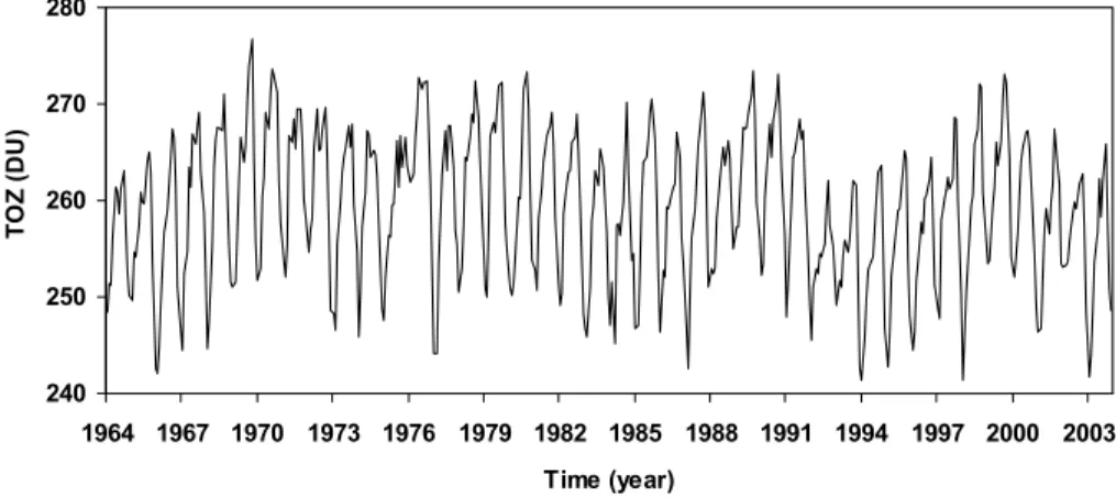
We begin with the investigation of the time scaling of the TOZ fluctuations over the trop-ical and mid-latitudinal zones of both Hemispheres. Figure 1 shows the monthly mean TOZ values over the belt 25◦S–25◦N as derived from the daily TOZ observations of 5

the WMO Dobson Network (WDN) during 1964–2004. Inspection of Fig. 1 shows that this time series is apparently non-stationary, and includes both periodic and aperiodic fluctuations.

We start the analysis of this time series by asking if the TOZ value in a given instant has any correlation with the TOZ in a later time, i.e. if TOZ time series exhibits long-10

range correlations. This question stems from the observation that many environmental quantities have values that remain residually correlated with one another even after many years (long-range dependence). Interestingly, the correlation function of the TOZ time series over tropics (not shown) decays more slowly than the corresponding expo-nential one. The departure from the expoexpo-nential fit becomes more pronounced towards 15

the low frequencies. Moreover, the determination of the power spectrum is hampered by large statistical uncertainties if one goes to low frequencies e.g. the quasi-biennial oscillation (QBO, with period ∼2-yr), and the 11-yr solar cycle.

To reliably gain insight into this problem, we deseasonalize the data (to avoid ob-scuring of a possible scaling behaviour from the long-term trend and various frequency 20

peaks induced from the well known cycles) (Hu et al., 2001). We then analyze the deseasonalized TOZ (D-TOZ) data of Fig. 1, using DFA.

In Fig. 2b, a log-log plot of the root-mean-square fluctuation function F_d(∆t)=F(n) is

shown, by applying the first order DFA (DFA-1) to the D-TOZ data derived from WDN, over the belt 25◦S–25◦N. Since, α=1.1(±0.04), we conclude that TOZ fluctuations over 25

the tropics exhibit persistent long-range correlations (1/f noise-like) for the interval time ranging from about 4 months to 11 years. The long-range correlations obtained do not signify the presence of cycles with definite periodicities (i.e. as described in Camp et al.,

(8)

ACPD

6, 4325–4340, 2006

Full Screen / Esc

2003), but rather the existence of dynamical links between long and short time-scale behavior.

Next, we examine the extra-tropics and the mid-latitude zone, and specifically the TOZ data of WDN for the latitude belts 25◦N–60◦N, 25◦S–60◦S during 1964–2004. By employing the DFA-1, the analysis of the D-TOZ data of 25◦N–60◦N shows that, 5

once again, persistent long-range correlations exist. According to Fig. 2a, since

α₁=1.22±0.04 (for time scales shorter than about 2 years) the correlations in TOZ

fluc-tuations exhibit “stronger memory” compared to that of α₂=0.63±0.04 (for time scales from about 2 to 11 years).

The results obtained from the application of the DFA-1 method to the D-TOZ values 10

in the latitude belt 25◦S–60◦S are depicted in Fig. 2c, where again, persistence of TOZ fluctuations is observed. In particular, for time scales shorter than about 2 years,

α₁=1.11±0.02, while for longer time scales, α₂=0.64±0.06. Thus, the tropics exhibit

stronger persistence at long time scales than the extratropics, but approximately equiv-alent persistence at short time scales (Varotsos, 2005).

15

The fact that in both extratropical bands, the persistence of ozone fluctuations changes character at about 2 years, suggests some connection with the QBO. The result suggests that for timescales longer than 2 years, there is little dynamical mem-ory for ozone fluctuations in the extratropics. It is therefore interesting and puzzling that this change in character of the persistence does not appear in the tropics, where 20

QBO dynamics originate, and where positive TOZ deviations are observed to occur a few months before the maximum westerlies at 50 hPa (WMO, 2003). Similar to the above-mentioned results for the TOZ variability over extra-tropics and mid-latitudes are also found by applying the DFA-1 method to the D-TOZ data derived from the Total Ozone Mapping Spectrometer (TOMS) observations (not shown).

25

To check the above-discussed results, the DFA-l method was applied to the same D-TOZ time series. The results obtained did not show any significant deviations from DFA-1. As a further check, we investigated whether the persistence found in TOZ time series stems from the values of TOZ by themselves and not from their time evolution.

(9)

ACPD

6, 4325–4340, 2006

Full Screen / Esc

EGU Therefore, we applied DFA-1 to randomly shuffled TOZ data over the tropics. This gave

α=0.51±0.01. Thus, the persistence in TOZ time series stems from the sequential

ordering of the TOZ values and is not a result of the distribution of the TOZ values. Similar results were also obtained for the TOZ time series over extra-tropics and mid-latitudes in both Hemispheres.

5

In addition, an effort has been made to detect whether the persistence observed in the TOZ data over the tropics and mid-latitudes also characterizes the ozone layer over the polar and arctic region (as defined in Hudson et al., 2003). To this end, we constructed a mixed TOZ time series consisting of TOMS observations, when WDN had no available observations for the region of interest, and vice-versa. The application 10

of the same analysis described above led to α=0.83±0.02 for the polar region, and to

α=0.81±0.03 for the arctic region. Similar results were also obtained for the Southern

Hemisphere. Nevertheless, the latter must be considered with caution, because at these regions the number of WDN stations is very limited and TOMS data are only available when sunlight is present.

15

Furthermore, the log-log plot derived from the application of DFA-1 on the global D-TOZ data reveals that α=1.1±0.02, suggesting that strong persistence in the tropics and mid-latitudes discussed above dominates the variability of the global ozone layer. In summary, the TOZ fluctuations over the tropics, extra-tropics, and mid-latitudes of both Hemispheres, as well as globally, exhibit persistent long-range correlations for all 20

time lags between about 4 months–11 years. Over the extra-tropics, this persistence becomes weaker for time lags between about 2–11 years. These findings are consis-tent with the preliminary results presented in Varotsos (2005).

3.2 Time scaling of the tropospheric temperature fluctuations

We next examine the existence of time scaling of the TBT fluctuations, an atmospheric 25

parameter that is often used to quantify global warming. The data used are the passive microwave temperature soundings from the Microwave Sounding Units (MSU chan-nel 2 from the satellites TIROS-N, NOAA-6 to NOAA-12, and NOAA-14) and the

(10)

Ad-ACPD

6, 4325–4340, 2006

Full Screen / Esc

vanced Microwave Sounding Units (AMSU channel 5 from the satellites NOAA-15 to NOAA-17 and AQUA) for the time period 1978–2004. A detailed description of the multi-satellite data analysis and the development technique of the time series of the bias-corrected globally averaged daily mean (pentad averaged) TBT is given in Vin-nikov and Grody (2003). It should be recalled that the MSU channel 2 brightness tem-5

perature measurements have been used during the last fifteen years as an indicator of air temperature in the middle troposphere (Vinnikov and Grody, 2003). Furthermore, to account for the effects of dynamical perturbations on TOZ, the TBT is often used as an index of dynamical variability (Chandra et al., 1996).

In Fig. 3b, a log-log plot of the function F_d(∆t) is shown, by employing the DFA-1 to

10

the D-TBT time series averaged in pentads of days over the belt 25◦S–25◦N. Since

α₁=1.13±0.04 (for time scales shorter than about 2 years) the fluctuations in TBT

exhibit long range correlations, whilst for time scales from about 2 to 7 years (e.g. El Nino-Southern Oscillation) they obey a random walk (α₂=0.50±0.04). The crossover point (at about 2 years) was defined as that point where the errors in both linear best 15

fits are minimized.

We now focus on the extra-tropics and the mid-latitude zone, e.g. 25◦N–60◦N and 25◦S–60◦S. The application of the DFA-1 to the D-TBT data over both belts (Figs. 3a, c) reveals that long-range power-law correlations exist in both Hemispheres, for the interval time ranging from about 20 days to 7 years, with α=0.80±0.01. Thus the global 20

TBT fluctuations exhibit long-range persistence. These results were confirmed by DFA-2 to DFA-7 analysis yielding α-values ranging from 0.78 to 0.86. We again confirmed the persistence found above by applying DFA-1 on the shuffled TBT anomalies, which again showed no persistent fluctuations.

4 Conclusions

25

We find opposite results for mid-tropospheric temperature and for ozone fluctuations. For ozone fluctuations, persistence at long time scales is strongest in tropics, but

(11)

ACPD

6, 4325–4340, 2006

Full Screen / Esc

EGU weaker in latitude, while temperature fluctuations show strong persistence in

mid-latitudes, and random walk in the tropics. Various mechanisms might account for the differences we have detected in the persistence in temperature and ozone. Greater persistence is in general a result of either stronger positive feedbacks or larger iner-tia. Thus, the reduced slope of the power distribution of temperature in the tropics at 5

long time scales, compared to the slope in the mid-latitudes could be connected to the poleward increase in climate sensitivity (due to latitude-dependent climate feedbacks) predicted by the global climate models. However this prediction applies to surface tem-perature, rather than to mid-tropospheric temperatures, which are expected to increase more or less uniformly with latitude.

10

We can rationalize the latitude dependence of the persistence in ozone fluctuations as follows. Zonal mean TOZ fluctuations in the mid-latitudes are governed largely by motions of the jet stream, which marks the boundary between low tropopause heights on the poleward side (and more TOZ) and higher tropopause heights (and less TOZ) on the tropical side (Hudson et al., 2003). Such variations might be expected to show rel-15

atively low persistence beyond time scales of a few months (or else seasonal weather prediction would be easier). Thus, the difference in persistence patterns between ozone and temperature could arise because the TOZ distribution is more closely tied to gradients in temperature (which are associated with the jet position), than to the tem-perature itself. Column ozone fluctuations in tropics are more closely tied to the QBO 20

and ENSO (Camp et al., 2003), and so would be expected to exhibit some persistence at time scales of more than two years.

At present, although many coupling mechanisms between ozone and temperature are known, the net effect of the interactions and feedbacks is only poorly understood and quantified. Our analysis has thus revealed dynamical features of the atmosphere 25

that are not simple to explain. Such features present appealing targets for model-data intercomparison, since models will not have been tuned to present them. Comparison of these results with similar analysis of model output should provide a robust test of the fidelity of the model dynamics to atmospheric dynamics, and could improve

(12)

predic-ACPD

6, 4325–4340, 2006

Full Screen / Esc

tion of global warming and future column ozone depletion (or recovery) under different climate change and halogen loading scenarios.

Acknowledgements. The TOMS data were produced by the Ozone Processing Team at NASA’s

Goddard Space Flight Center. The ground-based data are credited to V. Fioletov, Experimental Studies Division, Air Quality Research Meteorological Service of Canada. MSU/AMSU data

5

were kindly provided by K. Y. Vinnikov, Department of Atmospheric and Oceanic Science, Uni-versity of Maryland, USA.

References

Ausloos, M. and Ivanova, K.: Power-law correlations in the southern-oscillation-index fluctua-tions characterizing El Nino, Phys. Rev. E, 63, 047201, 2001.

10

Brandt, J., Christensen, J., Frohn, L. M., and Berkowicz, R.: Air pollution forecasting from regional to urban street scale – implementation and validation for two cities in Denmark, Phys. Chem. Earth, 28(8), 335–344, 2003.

Camp, C. D., Roulston, M. S., and Yung, Y. L.: Temporal and spatial patterns of the interannual variability of total ozone in the tropics, J. Geophys. Res., 108(D20), 4643, 2003.

15

Chandra, S., Varotsos, C., and Flynn, L. E.: The mid-latitude total ozone trends in the northern hemisphere, Geophys. Res. Lett., 23, 555–558, 1996.

Chen, Z., Ivanov, P. C., Hu, K., and Stanley, H. E.: Effect of nonstationarities on detrended fluctuation analysis, Phys. Rev. E, 65, 041107, 2002.

Chen, Z., Hu, K., Carpena, P., Bernaola-Galvan, P., Stanley, H. E., and Ivanov, P. C.: Effect of

20

nonlinear filters on detrended fluctuation analysis, Phys. Rev. E, 71, 011104, 2005.

Collette, C. and Ausloos, M.: Scaling analysis and evolution equation of the North Atlantic oscillation index fluctuations, ArXiv:nlin.CD/0406068 29, 2004.

Crutzen, P. J., Lawrence, M. G., and Poschl, U.: On the background photochemistry of tropo-spheric ozone, Tellus A, 51(1), 123–146, 1999.

25

Dameris, M., Grewe, V., Ponater, M., Deckert, R., Eyring, V., Mager, F., Matthes, S., Schnadt, C., Stenke, A., Steil, B., Bruhl, C., Giorgetta, M. A.: Long-term changes and variability in a transient simulation with a chemistry-climate model employing realistic forcing, Atmos. Chem. Phys., 5, 2121–2145, 2005.

(13)

ACPD

6, 4325–4340, 2006

Full Screen / Esc

EGU

Ebel, A.: Evaluation and reliability of meso-scale air pollution simulations, Lect. Notes Comput. Sci., 2179, 255–263, 2001.

Galmarini, S., Steyn, D. G., and Ainslie, B.: The scaling law relating world point-precipitation records to duration, Int. J. Climatol., 24(5), 533–546, 2004.

Grytsai, A., Grytsai, Z., Evtushevsky, A., and Milinevsky, G.: Interannual variability of planetary

5

waves in the ozone layer at 65 degrees S, Int. J. Remote Sens., 26(16), 3377–3387, 2005. Hu, K., Ivanov, P. C., Chen, Z., Carpena, P., and Stanley H. E.: Effect of trends on detrended

fluctuation analysis, Phys. Rev. E, 64, 011114, 2001.

Hudson, R. D., Frolov, A. D., Andrade, M. F., and Follette, M. B.: The total ozone field separated into meteorological regimes. Part I: Defining the regimes, J. Atmos. Science, 60, 1669–1677,

10

2003.

Kantelhardt, J. W., Zschiegner, S. A., Koscielny-Bunde, E., Havlin, S., Bunde, A., and Stanley, H. E.: Multifractal detrended fluctuation analysis of nonstationary time series, Physica A, 316(1–4), 87–114, 2002.

Kirk-Davidoff, D. B., Anderson, J. G., Hintsa, E. J., and Keith, D. W.: The effect of climate

15

change on ozone depletion through stratospheric H₂O, Nature, 402, 399, 1999.

Kondratyev, K. and Varotsos, C.: Atmospheric ozone variability: Implications for climate change, human health and ecosystems, Springer, New York, 2000.

Lawrence, M. G., Crutzen, P. J., Rasch, P. J., Eaton, B. E., and Mahowald, N. M.: A model for studies of tropospheric photochemistry: Description, global distributions, and evaluation, J.

20

Geophys. Res.-Atmos., 104, 26 245–26 277, 1999.

Peng, C. K., Buldyrev, S. V., Havlin, S., Simons, M., Stanley, H. E., and Goldberger, A. L.: Mosaic organization of DNA nucleotides, Phys. Rev. E, 49(2), 1685–1689, 1994.

Sander, R.: Modeling atmospheric chemistry: Interactions between gas-phase species and liquid cloud/aerosol particles, Surv. Geophys., 20(1), 1–31, 1999.

25

Stanley, E.: Scaling, universality, and renormalization: Three pillars of modern critical phenom-ena, Rev. Mod. Phys., 71(2), S358–S366, 1999.

Stohl, A., Cooper, O. R., and James, P.: A cautionary note on the use of meteorological analysis fields for quantifying atmospheric mixing, J. Atmos. Sci., 61(12), 1446–1453, 2004.

Talkner, P. and Weber, R. O.: Power spectrum and detrended fluctuation analysis: Application

30

to daily temperatures, Phys. Rev. E, 62(1), 150–160, 2000.

Varotsos, C.: Modern computational techniques for environmental data: Application to the global ozone layer, Proceedings of the ICCS 2005 in Lect. Notes Comput. Sci., 3516, 504–

(14)

ACPD

6, 4325–4340, 2006

Full Screen / Esc

510, 2005.

Varotsos, P. A., Sarlis, N. V., and Skordas, E. S.: Long-range correlations in the electric signals that precede rupture: Further investigations, Phys. Rev. E, 67, 21 109, 2003a.

Varotsos, P. A., Sarlis, N. V., and Skordas, E. S.: Attempt to distinguish electric signals of a dichotomous nature, Phys. Rev. E, 68, 031106, 2003b.

5

Varotsos, C., Ondov, J., and Efstathiou, M.: Scaling properties of air pollution in Athens, Greece, and Baltimore, Maryland, Atmos. Environ., 39(22), 4041–4047, 2005.

Vinnikov, K. Y. and Grody, N. C.: Global warming trend of mean tropospheric temperature observed by satellites, Science, 302, 269–272, 2003.

Weber, R. O. and Talkner, P.: Spectra and correlations of climate data from days to decades, J.

10

Geophys. Res., 106, 20 131–20 144, 2001.

World Meteorological Organization: Scientific assessment of ozone depletion 2002, Rep. 47, World Meteorol. Organ., Geneva, Switzerland, 2003.

(15)

ACPD

6, 4325–4340, 2006

Full Screen / Esc

Printer-friendly Version Interactive Discussion EGU 240 250 260 270 280 1964 1967 1970 1973 1976 1979 1982 1985 1988 1991 1994 1997 2000 2003 Time (year) TO Z ( D U )

Fig. 1. TOZ mean monthly values (in Dobson Units – DU) during 1964–2004, over the belt

25◦S–25◦N derived from the WMO Dobson Network (100 DU=1 mm thickness of pure ozone on the Earth’s surface).

(16)

ACPD

6, 4325–4340, 2006

Full Screen / Esc

Printer-friendly Version Interactive Discussion TOZ 25°N-60°N y = 1.22x - 0.41 R2_{= 0.984} y = 0.63x + 0.35 R2_{= 0.942} 0 0.2 0.4 0.6 0.8 1 1.2 1.4 1.6 1.8 0 1 2 3 log∆t logF d TOZ 25°S-25°N y = 1.10x - 0.67 R2_{= 0.995} -0.2 0 0.2 0.4 0.6 0.8 1 1.2 1.4 1.6 1.8 0 1 2 3 log∆t logF d TOZ 25°S-60°S y = 1.11x - 0.33 R2_{= 0.997} y = 0.64x + 0.34 R2_{= 0.90} 0 0.2 0.4 0.6 0.8 1 1.2 1.4 1.6 1.8 2 0 1 2 3 log∆t lo g Fd (a) (b) (c) TOZ 25°N-60°N y = 1.22x - 0.41 R2_{= 0.984} y = 0.63x + 0.35 R2_{= 0.942} 0 0.2 0.4 0.6 0.8 1 1.2 1.4 1.6 1.8 0 1 2 3 log∆t logF d TOZ 25°S-25°N y = 1.10x - 0.67 R2_{= 0.995} -0.2 0 0.2 0.4 0.6 0.8 1 1.2 1.4 1.6 1.8 0 1 2 3 log∆t logF d TOZ 25°S-60°S y = 1.11x - 0.33 R2_{= 0.997} y = 0.64x + 0.34 R2_{= 0.90} 0 0.2 0.4 0.6 0.8 1 1.2 1.4 1.6 1.8 2 0 1 2 3 log∆t lo g Fd (a) (b) (c) TOZ 25°N-60°N y = 1.22x - 0.41 R2_{= 0.984} y = 0.63x + 0.35 R2_{= 0.942} 0 0.2 0.4 0.6 0.8 1 1.2 1.4 1.6 1.8 0 1 2 3 log∆t logF d TOZ 25°S-25°N y = 1.10x - 0.67 R2_{= 0.995} -0.2 0 0.2 0.4 0.6 0.8 1 1.2 1.4 1.6 1.8 0 1 2 3 log∆t logF d TOZ 25°S-60°S y = 1.11x - 0.33 R2_{= 0.997} y = 0.64x + 0.34 R2_{= 0.90} 0 0.2 0.4 0.6 0.8 1 1.2 1.4 1.6 1.8 2 0 1 2 3 log∆t lo g Fd (a) (b) (c)

Fig. 2. Log-log plot of the TOZ root-mean-square fluctuation function (Fd ) versus temporal

interval∆t (in months) for deseasonalized TOZ values, observed by the WMO Dobson Network over the tropics(b), and mid-latitudes of both Hemispheres (a, c) during 1964–2004 (crossover

(17)

ACPD

6, 4325–4340, 2006

Full Screen / Esc

Printer-friendly Version Interactive Discussion EGU TRT 25°N-60°N y = 0.80x - 1.25 R2_{= 0.996} -1 -0.5 0 0.5 1 0 1 2 3 log∆t logF d TRT 25°S-25°N y = 1.13x - 1.82 R2_{= 0.998} y = 0.50x - 0.31 R2_{= 0.934} -1.5 -1 -0.5 0 0.5 1 5 0 1 2 3 log∆t lo g Fd TRT 25°S-60°S y = 0.80x - 1.42 R2_{= 0.994} -1.5 -1 -0.5 0 0.5 1 5 0 1 2 3 4 log∆t lo g F d 1.5 (a) (b) _1. (c) 1. 4 4 TRT 25°N-60°N y = 0.80x - 1.25 R2_{= 0.996} -1 -0.5 0 0.5 1 0 1 2 3 log∆t logF d TRT 25°S-25°N y = 1.13x - 1.82 R2_{= 0.998} y = 0.50x - 0.31 R2_{= 0.934} -1.5 -1 -0.5 0 0.5 1 5 0 1 2 3 log∆t lo g Fd TRT 25°S-60°S y = 0.80x - 1.42 R2_{= 0.994} -1.5 -1 -0.5 0 0.5 1 5 0 1 2 3 4 log∆t lo g F d 1.5 (a) (b) _1. (c) 1. 4 4 TRT 25°N-60°N y = 0.80x - 1.25 R2_{= 0.996} -1 -0.5 0 0.5 1 0 1 2 3 log∆t logF d TRT 25°S-25°N y = 1.13x - 1.82 R2_{= 0.998} y = 0.50x - 0.31 R2_{= 0.934} -1.5 -1 -0.5 0 0.5 1 5 0 1 2 3 log∆t lo g Fd TRT 25°S-60°S y = 0.80x - 1.42 R2_{= 0.994} -1.5 -1 -0.5 0 0.5 1 5 0 1 2 3 4 log∆t lo g F d 1.5 (a) (b) _1. (c) 1. 4 4

Fig. 3. Log-log plot of the TBT root-mean-square fluctuation function (Fd ) versus temporal

in-terval∆t (averaged in pentads of days) for deseasonalized TBT (mid-tropospheric temperature) values, observed by the multi-satellite instrumentation over the tropics(b), and mid-latitudes of