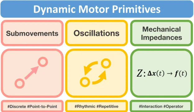
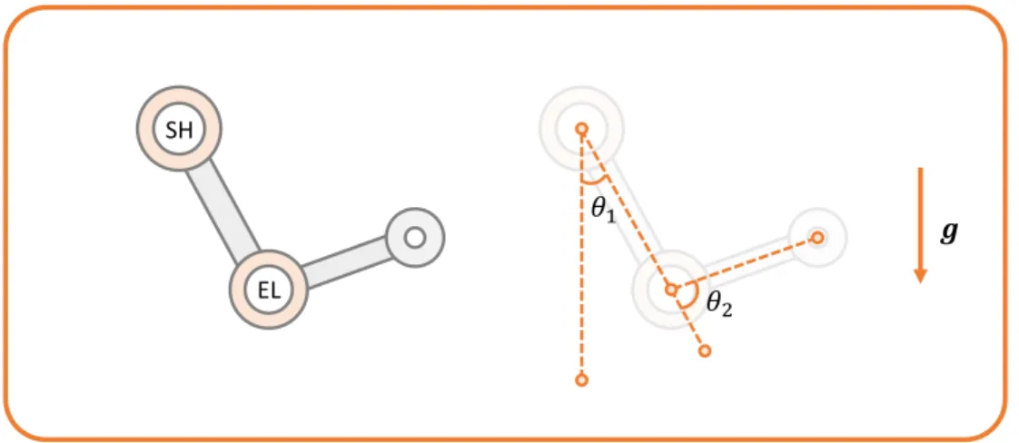
Dynamic primitives facilitate manipulating a whip

In order to address complex large-scale shoreline shapes, the LX-Shore model computes the time evolution of the sediment fraction F (ranging from 0 to 1) inside a plan-view grid

Control of a Robotic Swarm Formation to Track a Dynamic Target with Communication Constraints: Analysis and

L’archive ouverte pluridisciplinaire HAL, est destinée au dépôt et à la diffusion de documents scientifiques de niveau recherche, publiés ou non, émanant des

• Implementar controles y registros del dinero que aportan los comunitarios, así como de las salidas de dinero para el pago de las actividades que se realizan en

Thus, two experiments are used: the inversed perforation test based on the Hopkinson bar measurement technique, and the direct perforation test coupled with digital

Conformément aux principes énoncés par la "Budapest Open Access Initiative"(BOAI, 2002), l'utilisateur du site peut lire, télécharger, copier, transmettre, imprimer, chercher

On appelle primitive d'une fonction f sur un intervalle I, toute fonction F définie et dérivable sur I, dont la dérivée est

The present paper aims to fill this lack, giving numerical results for the static torque on a Savonius rotor, and presenting the dynamic behavior in reference to the results