HAL Id: hal-02734892
https://hal-brgm.archives-ouvertes.fr/hal-02734892
Submitted on 18 Nov 2020HAL is a multi-disciplinary open access archive for the deposit and dissemination of sci-entific research documents, whether they are pub-lished or not. The documents may come from teaching and research institutions in France or abroad, or from public or private research centers.
L’archive ouverte pluridisciplinaire HAL, est destinée au dépôt et à la diffusion de documents scientifiques de niveau recherche, publiés ou non, émanant des établissements d’enseignement et de recherche français ou étrangers, des laboratoires publics ou privés.
A reduced-complexity shoreline change model combining
longshore and cross-shore processes: The LX-Shore
model
Arthur Robinet, Déborah Idier, Bruno Castelle, Vincent Marieu
To cite this version:
Arthur Robinet, Déborah Idier, Bruno Castelle, Vincent Marieu. A reduced-complexity shoreline change model combining longshore and cross-shore processes: The LX-Shore model. Environmental Modelling and Software, Elsevier, 2018, 109, pp.1-16. �10.1016/j.envsoft.2018.08.010�. �hal-02734892�
1
A reduced-complexity shoreline change model combining longshore and
cross-shore processes: the LX-Shore model
Arthur Robinet1,2,3, Déborah Idier1, Bruno Castelle2,3, Vincent Marieu2,3
1 Bureau de Recherche en Géologie Minière, 3 avenue Claude Guillemin, Orléans, France
2 CNRS, UMR 5805 EPOC, Allée Geoffroy Saint-Hilaire, Pessac, France
3 Univ. Bordeaux, UMR 5805 EPOC, Allée Geoffroy Saint-Hilaire, Pessac, France
Corresponding Author Arthur Robinet: [email protected]
Abstract
A reduced-complexity numerical model, LX-Shore, is developed to simulate shoreline evolution along wave-dominated sandy coasts. The model can handle any sandy shoreline geometries (e.g. sand spits, islands), including non-erodible areas such as coastal defenses and headlands, and is coupled with a spectral wave model to cope with complex nearshore wave fields. Shoreline change is primarily driven by the gradients in total longshore sediment transport and by the cross-shore transport owing to variability in incident wave energy. Application to academic cases and a real coast highlights the potential of LX-Shore to simulate shoreline change on timescales from hours (storm) to decades with low computational cost. LX-Shore opens new perspectives in terms of knowledge on the primary mechanisms locally driving shoreline change and for ensemble-based simulations of future shoreline evolution.
Keywords
Numerical model; shoreline change; sandy coasts; cross-shore transport; longshore transport
1. Introduction
In the context of global climate change and population growth, the littoral region is a particular hot-spot that is becoming increasingly topical and politically sensitive worldwide in a context of widespread erosion (see e.g. Bird, 1985). Over the last couple of decades, a number of complex hydrodynamic-based models
2
(resolving waves, currents, sediment transport and bed evolution in space and time) have been developed to simulate and further predict wave-dominated morphological changes including shoreline evolution (e.g. Lesser et al., 2004). Although these models have been found to simulate morphological changes with fair accuracy on short timescales (say from hours to weeks, e.g. Roelvink et al., 2009, for storm-driven erosion), they cannot be used to predict shoreline evolution on long timescales (i.e. months, years, decades). In essence, all these fully coupled and strongly nonlinear hydrodynamic-based morphodynamic models contain misspecifications of the physics. For instance, sand stirring accounting for breaking-wave-induced turbulence as a surface boundary condition (e.g. Grasso et al., 2012) and swash zone sediment transport processes (Masselink and Puleo, 2006) are not accurately or properly considered in these hydrodynamic-based models. Other key processes, such as depth-induced breaking wave energy dissipation which is the primary driving force to nearshore circulation and resulting sand transport, are addressed through parametrizations that contain errors, even though small (e.g. Ruessink et al., 2003). These misspecifications rapidly cascade up through the scales resulting in an inescapable build-up of errors and unreliable simulations on long timescales. In addition, complex hydrodynamic-based morphodynamic models are too computationally consuming to enable long-term simulations of shoreline change on wave-dominated coasts (e.g. Daly et al., 2014), which is even more true on the spatial scales of kilometers to tens of kilometers. In contrast, reduced-complexity models can lead to more reliable long-term evolution than do parameterizations of much smaller-scale processes in complex hydrodynamic-based models, as evidenced in many geomorphological systems (Murray, 2007).
As far as coastal change is concerned, one can regard localized short-term morphological variations (e.g. localized changes caused by rip currents) as negligible perturbations superimposed on the main trend of shoreline evolution. The resulting fundamental assumption that allows reducing the model complexity is that erosion or accretion of a beach results in a pure translation of beach profile. In such models, hereafter referred to as one-line models, the bottom profile moves in parallel to itself without changing shape, which dramatically decreases the computational cost and enables addressing shoreline variability on spatial scales of up to tens and hundreds of kilometers (e.g. Ashton and Murray, 2006a). Over these spatial scales and away from tidal inlets and estuaries, shoreline change along most wave-dominated coasts is driven by both longshore and cross-shore wave-driven processes acting with respective contributions that vary according to local wave climate and geological settings. Alongshore gradients in longshore sand transport have long been assumed as the primary shoreline change driver on long timescales, overwhelming the impact of sea-level rise (Cowell et al., 1995). However, there is also evidence that cross-shore processes at the scale of changes in wave regime (e.g. hours to days) controls shoreline variability on timescales greater than years. For instance, wave-driven beach profile dynamics, with rapid storm-driven erosion and slow post-storm
3
recovery, cascade up through the scales and explain interannual shoreline variability on cross-shore sand transport dominated coasts (e.g. Robinet et al., 2016). In addition, storm-driven-overwash (Donnelly et al., 2006) can also cause lasting erosion at event-scale that cumulates over the time, inducing long-term trends of coastal retreat along gentle sandy coasts such as barrier islands (Leatherman, 1979; Lorenzo-Trueba and Ashton, 2014). The respective contributions of cross-shore and alongshore processes to shoreline variability are site specific and subject to debate, as for instance along the ubiquitous embayed beaches bounded by headlands and/or coastal structures (Harley et al., 2015). Accounting for both cross-shore and alongshore processes in a shoreline evolution numerical model is a necessary requirement to understand the primary drivers of shoreline change on wave-dominated sandy coasts and to further predict future changes.
Until now, cross-shore and alongshore processes have been mostly addressed in isolation (Ashton and Murray, 2006a; Davidson et al., 2013; Hanson, 1989; Larson et al., 2016; Splinter et al., 2014; Yates et al., 2009). In addition, simplified wave models have often been used for shoreline change modeling to reduce computational cost, which prevents the model application to complex coasts where offshore and/or nearshore wave refraction and diffraction strongly affects breaking wave characteristics alongshore. A fundamental step to increase our understanding of shoreline change and prediction capabilities from the timescales of hours (i.e. storm) to decades is to combine cross-shore and alongshore processes into a single reduced-complexity shoreline model accounting for the complexity of offshore and nearshore wave transformation. In this paper, we develop such a one-line model to simulate short- to long-term wave-driven shoreline change with reasonable computation time (one day of computation time corresponds to 103-104
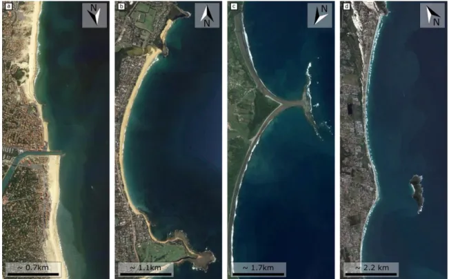
days of real time for a 4-km-long beach). The model is designed to address shoreline variability on a wide range of wave-dominated sandy coasts including headlands and/or coastal structures to cover the wide spectrum of coastal plan-view shapes (Fig. 1). The general background on the existing shoreline change models is presented in Section 2. The development of our new shoreline change numerical model is detailed in Section 3 together with the primary physical assumptions, before being applied to a series of synthetic cases in Section 4. A discussion on the model assumptions, limitations and capabilities as well as perspectives on future developments and applications are presented in Section 5. Conclusions are drawn in Section 6.
4
Figure 1. Examples of complex shoreline plan-view shapes enforced by the inherited geology (e.g. headlands, offshore islands) or coastal hard structures. a Hossegor-Capbreton beaches, France. b Narrabeen beach, Australia. c
Punta Uvita, Costa Rica. d Campeche beach, Brazil. Source: Google Earth imagery.
2. Shoreline change models
2.1. Cross-shore-transport driven shoreline change
Shoreline changes driven by cross-shore processes are essentially controlled by the time variability of wave energy arriving at the coast. It is now well established that during storms, on timescales from hours to days, high-energy breaking waves drive strong offshore-directed currents referred to as undertow that rapidly erode the beach and transport sediment seaward (e.g. Gallagher et al., 1998). The horizontal and vertical asymmetries in the wave free-surface over the shoaling and surf zones induce an asymmetry between the onshore and offshore directed near-bed orbital velocity distributions, with a narrower distribution of higher near-bed orbital velocities directed onshore. Because the sediment transport is a non-linear function of the water velocity, this asymmetry causes locally a net onshore-directed sediment transport that dominates the cross-shore transport during post-storm periods associated with low-energy breaking waves, on timescales from days to weeks up to months, resulting in a slow accretion of the beach (Hoefel and Elgar, 2003). Although hydrodynamic-based beach profile models can simulate these dynamics in the nearshore (e.g. Dubarbier et al., 2015; Fernández-Mora et al., 2015; Kuriyama et al., 2012; Ruessink et al., 2007), the swash
5
zone dynamics and, in turn, shoreline evolution are poorly resolved. Instead, a wealth of simpler empirical equilibrium-based shoreline models have recently been developed based on the work of Wright and Short (1984). These models, which assume that the present shoreline position is determined by the recent history of the wave field and/or the shoreline position, read:
eq
dS
C W
dt
(1)where S is the shoreline position, C is a time varying change rate of the shoreline position depending on wave conditions, and ΔWeq the disequilibrium between the present and equilibrium conditions which can be
expressed in terms of shoreline position (e.g. Yates et al., 2009) or wave history (e.g. Davidson et al., 2013, with the ShoreFor model). In other words, these models describe the rate of cross-shore shoreline change as a function of this disequilibrium and the magnitude of forcing available to move the sand. These reasonably simple equilibrium-based empirical shoreline models have been found to simulate shoreline behavior on timescales of days to years, with low computational cost, at many cross-shore dominated sandy beaches, and with satisfactory results (Castelle et al., 2014; Davidson et al., 2013, 2010; Davidson and Turner, 2009; Frazer et al., 2009; Jara et al., 2015; Miller and Dean, 2004; Splinter et al., 2017, 2014; Yates et al., 2011, 2009).
It is generally acknowledged that monitoring programs of at least two years with shorelines sampled at least monthly are sufficient to determine initial estimates of calibration coefficients and to hindcast short-term (1-5 years) shoreline variability using empirical equilibrium-based shoreline models (Splinter et al., 2013). However, more recent work suggests that longer periods should be used to maximize the chance to include outstanding winters and/or change in the seasonality of storms that can affect calibration parameters and, in turn, the mode of shoreline variability (Splinter et al., 2017).
It is important to note that such simple equilibrium-based empirical shoreline models neglect the overwash mechanisms that can impact long-term shoreline change (Lorenzo-Trueba and Ashton, 2014). Along gentle sandy coasts, such as barrier islands, beach sediment can be transported landward under storm-driven overwash, causing losses of sediment in the active upper shoreface (Donnelly et al., 2006). In that case, the assumption that the sediment eroded on the upper beach during storms deposits seaward before being slowly transported back shoreward during milder wave conditions is not tenable. The above-mentioned post-storm recovery process is then expected to be weakened (Larson et al., 2016) and application of equilibrium-based
6
cross-shore shoreline models in these environments must be performed with caution (Lorenzo-Trueba and Ashton, 2014). Where overwash contribution dominates the shoreline variability alternative modeling approaches must be used (e.g. Ashton and Murray, 2006a; Jiménez and Sánchez-Arcilla, 2004; Larson et al., 2016; Lorenzo-Trueba and Ashton, 2014).
2.2. Longshore-transport driven shoreline change
The longshore-transport one-line approach has long been used for coastal engineering applications (Durand, 2001; Hanson, 1989; Larson et al., 2002; Szmytkiewicz et al., 2000). The total longshore sediment transport (Ql) is computed by integrating the longshore sediment transport along the cross-shore profile down to the
depth below which wave influence on the bottom profile evolution becomes negligible at the timescale of interest. This depth, known as the closure depth (Dc), defines the morphological active region of the
shoreface and can be computed according to the wave climate with empirical formulas for engineering purpose up to decades (Birkemeier, 1985; Hallermeier, 1980) or with theoretical formulations to deal with longer timescales (Ortiz and Ashton, 2016). Any gradient in total longshore sediment transport results in sediment deposition or erosion uniformly spread along the beach profile leading to a horizontal translation of the profile and, in turn, of the shoreline position. This concept, which was first introduced by Pelnard-Considère (1956), reads in a Cartesian reference system (x, y):
1
lc
dQ
dS
dt
D dx
(2)where the x-axis is aligned with the shoreline orientation, the y-axis is the perpendicular direction seaward and t is the time. The total longshore sediment transport Ql is typically computed using an empirical formula,
to be selected among the many different ones proposed in the literature (e.g. Bayram et al., 2007; Kamphuis, 1991; USACE, 1984). All these empirical formulations use breaking wave conditions as input, sometimes with the addition of the beach characteristics (Kamphuis et al. 1986). This simple approach was shown to simulate shoreline change with fair accuracy along a number of longshore-transport dominated coasts (e.g. Hanson, 1989; Larson et al., 2002; Pelnard-Considère, 1956). However, the limitations of this approach are primarily twofold: (1) multiple shoreline positions along the same y-axis is not allowed and (2) large shoreline curvature is incompatible with the assumptions in Eq. (2) (see Hurst et al., 2015; Kaergaard and Fredsoe, 2013a).
7
implemented a 2D cellular-based one-line model, the Coastal Evolution Model (CEM). The model framework consists in a 2D plan-view grid where each cell is filled with a fractional amount of sediment (F). A cell with a sediment fraction F = 1 (0) is fully dry (subaqueous), with the shoreline consisting of the line of cells with 0 < F < 1. At each time step, the fractional sediment contents of shoreline cells are adjusted according to the net sediment flux into or out of the cell. This pioneering approach allows addressing the longshore-transport driven dynamics of complex large-scale shoreline shapes, including for instance spits, islands and enclosed lakes. A major achievement performed with CEM has been to decipher the underlying mechanisms responsible for the formation and subsequent nonlinear evolution of shoreline instabilities under highly obliquely incident waves with academic cases (Ashton et al., 2009; Ashton and Giosan, 2011; Ashton and Murray, 2006b).
However, in the CEM model, as in most of the one-line models, wave propagation is computed using Snell’s law in combination with energy flux conservation, assuming linear and parallel isobaths. Such an approach shows satisfactory results with a shoreline configuration that is reasonably straight, but becomes unreliable when applied to complex coastline geometries (e.g. shoreline sandwaves, rugged and/or trained coasts) where wave energy focusing and spreading enforced at the shore by offshore wave refraction and diffraction are important to longshore sand transport and resulting shoreline change. Such simplifications also imply that there is no feedback between the 2D bathymetric changes induced by the shoreline evolution (e.g. bay and cape developments) and the waves, increasing the inaccuracy in the computation of wave energy focusing and spreading areas. This was demonstrated by, for instance, van den Berg et al. (2012) and Falqués et al. (2017) using the non-linear morphodynamic model Q2D-morfo. However, Q2D-morfo cannot handle complex shoreline plan-view shapes such as spits, islands and enclosed lakes. Building on this, Limber et al. (2017) proposed an improved version of the CEM, through the coupling with the nearshore spectral wave model SWAN (Booij et al., 1999; Ris et al., 1999). In this new version, named CEMSWAN, waves are propagated over an evolving bathymetry, with bathymetric changes occurring only locally, where the active beach profile translates due to shoreline changes. In the meantime, Kaergaard and Fredsoe (2013a, 2013b, 2013c) developed a one-line model more complex than the CEM, CEMSWAN and Q2D-morfo models. The model consists of the combination of a spectral wave model, a hydrodynamic model and a sediment transport model. The computation of the longshore sediment transport is performed over an unstructured finite volume mesh that is derived from the shoreline position using a complex advancing front technique. Based on a local coordinate system that follows the shoreline orientation, this model is able to simulate shoreline change along coastlines with large curvature, and multiple shoreline positions are allowed in any direction. This model, however, requires high computational resources (days of computation for simulating several years, Kaergaard, personal communication, 2015) which is prohibitive to perform sensitivity analysis or ensemble
8 forecasting.
Hurst et al. (2015) implemented a vector-based one-line model, the Coastal One-line Vector Evolution model (COVE), to investigate the relation between the long-term equilibrium plan-view shape of embayed beaches and the wave climate characteristics. Similarly to Kaergaard and Fredsoe (2013a), a local coordinate system following the shoreline orientation is used, and specific methods are implemented to ensure the sediment conservation when the shoreline evolves as well as accurate estimates of longshore transport between the different stretches of shoreline. In the COVE model, the resolution of the wave propagation and the sediment transport is simplified compared to the model of Kaergaard and Fredsoe (2013a), which allows exploring the long-term dynamics of the shoreline for academic embayed beaches with low computational cost, but limits the range of model application (especially when the plan-view coastal geometry is more complex). 2.3. Longshore-transport and cross-shore-transport driven shoreline change
Very recently, Vitousek et al. (2017) proposed a comprehensive approach with the development of a new transect-based one-line model (CoSMoS-COAST) for shoreline change including various processes acting at different temporal scales. In contrast with the other one-line models presented above, the model accounts for: (1) alongshore gradients in total longshore transport; (2) cross-shore processes induced by the disequilibrium in wave energy at the coast using the model of Yates et al. (2009); (3) shoreline retreat due to sea-level rise using the Bruun rule concept (Bruun, 1962); and (4) unresolved processes (e.g. fluvial inputs, cliff failure, aeolian transport) through an additional parameter acting as a long-term trend. A data assimilation procedure based on the extended Kalman filter is applied independently for each transect to adjust the first guess model free parameters using 15 years of measurements along the entire Southern California coast. The model shows good skill along this coast, but still has limitations (see section 5). For instance, there is no feedback between the shoreline (and associated bathymetry) and wave changes. Such a simplification holds only if the shoreline orientation does not change significantly.
Thus, to the authors’ knowledge, there is no one-line model accounting for both longshore and cross-shore processes, dealing with complex shorelines and non-erodible areas, including the feedback with the wave field using an advanced wave model, and with a low computational cost. Our new model aims at bridging this gap by coupling some of the conceptual approaches and modelling strategies presented above.
3. Model Development
As a first step, LX-Shore is designed for sandy coasts where overwash rarely occurs, such as beaches backed by high dunes or cliffs. LX-Shore consists of a 2D plan-view cellular-based one-line model where longshore
9
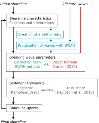
transport is resolved as in CEM, where cross-shore transport is driven by the disequilibrium in the wave conditions only (ShoreFor approach), and where the waves are fully coupled with the shoreline changes and computed using a spectral wave model. Additionally, specification of non-erodible areas is allowed (e.g. hard coastal defenses, headlands). The primary processes of LX-Shore and its overall structure are presented in Figures 2 and 3, respectively. In short, at each time step waves are propagated from the offshore boundaries to the coast where the breaking wave parameters are extracted. The breaking wave parameters are used to force the longshore and cross-shore sediment transport modules and, in turn, shoreline change through the sediment balance. The different components of the model are detailed below.
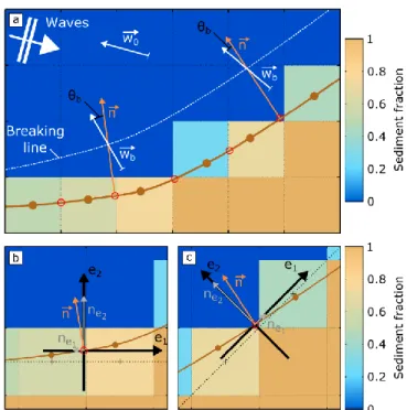
Figure 2. Overview of the features and processes integrated in the LX-Shore model. a Example of a plan-view coastal area used in the model. b Zoom showing where the longshore and cross-shore sediment transports are
10
Figure 3. LX-Shore model architecture. In black and blue: architecture in case the option of computing waves using SWAN is chosen. In black and red: architecture in case the option of computing waves using a direct formula is
chosen.
3.1. Sediment fraction and shoreline evolution
In order to address complex large-scale shoreline shapes, the LX-Shore model computes the time evolution of the sediment fraction F (ranging from 0 to 1) inside a plan-view grid where the shoreline consists of the line of cells with 0 < F < 1 having an edge contact with at least one water cell (Fig. 2). In essence, the sediment fraction is defined as the ratio between the sediment volume (Vs) contained by a cell and the
maximum sediment volume (Vs,max) this cell can contain (F = Vs/Vs,max). This sediment fraction is computed
on grid cells of a constant size (dxy), typically of the order of 10 to 100 m (Fig. 2). Assuming that shoreline change essentially results from a seaward or shoreward translation of a constant beach profile down to Dc,
the maximum sediment volume within a cell is Vs,max = dxy2Dc (Ashton and Murray, 2006a). At each time
step F is updated at each shoreline cell according to the incoming and outgoing sediment fraction caused by longshore and cross-shore transport:
11
where t is the time, Δt is the simulation time step, ΔFl and ΔFc are the sediment fraction variations from t to t+Δt induced by the longshore and cross-shore processes, respectively. Following Ashton et al. (2001), the
sediment fraction variation in the alongshore directionreads:
,in ,out ,max
(
l l)
l sQ
Q
F
t
V
(4)where Ql,in and Ql,out are the incoming and outgoing longshore sediment transport, respectively. Cross-shore
processes are included considering that the shoreline position fluctuates around a time-varying equilibrium position according to present and past wave conditions (Davidson et al., 2013). Although this approach implicitly accounts for the beach profile dynamics related to wave-driven cross-shore processes, it does not requires assumptions on Dc and the profile shape variability. Here, the beach profile is assumed to maintain
its shape and to translate simultaneously with shoreline change caused by the cross-shore processes. This allows straightforward conversion of predicted cross-shore-transport-driven shoreline change into variation in sediment fraction within the shoreline cells of the model. The sediment fraction variation resulting from cross-shore processes is given by:
c c S t F t dxy (5)
where ΔSc/Δt is the average shoreline change rate caused by cross-shore processes during Δt.
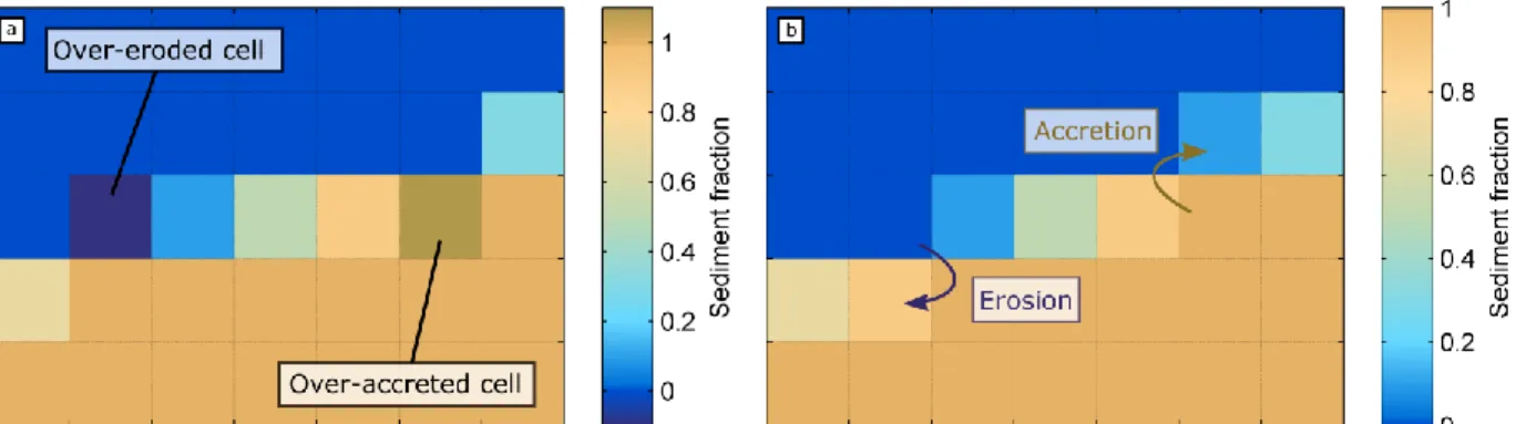
After the update, if the sediment fraction of shoreline cells becomes lower than 0 or greater than 1, a number of behavior laws are applied to the sediment fraction grid to ensure that 0 < F < 1 at the end of the process. The procedure consists of performing local adjustments of the sediment fraction with the surrounding cells. Any excess in sediment fraction is transferred to some specific neighboring water cells, while any deficit in sediment fraction is taken from some specific neighboring land cells. Figure 4 illustrates the application of the accretion and erosion laws for a simple sediment fraction grid configuration. The over-accreted shoreline cell (F > 1) spreads the sediment fraction excess into the most offshore water cell, while the over-eroded shoreline cell (F < 0) is fed by the most inland dry cell. Noteworthy, additional accretion and erosion rules were implemented to handle complex local shoreline shapes that are usually associated with various specific cell configurations (alignment of neighboring shoreline cells and positions of the surrounding water cells) in the sediment fraction grid (Robinet, 2017).
12
Figure 4. Illustration of empirical accretion and erosion laws applied to over-accreted (F > 1) and over-eroded (F < 0) shoreline cells, respectively. a before updating the sediment fraction grid. b after the update.
The longshore sediment transport is calculated at each boundary between two adjacent shoreline cells (green arrows in Fig. 2b) using the wave characteristics at breaking and the local shoreline orientation. This approach is conservative in terms of sediment budget since any volume of sediment removed from a shoreline cell is added to its downdrift shoreline cell. In contrast, the cross-shore sediment transport, which is calculated inside each shoreline cell (red double arrows in Fig. 2b), is not conservative as there are gains and losses of sediment volume according to the variability in incident wave energy at breaking. To account for non-erodible areas, we assume that the sediment fraction can be written F = FNE + FE with FNE and FE
the non-erodible and erodible sub-fractions, respectively. For each cell, FNE is a constant, defined by the
area of the cell overlapped by non-erodible areas, while FE is time dependent, and computed through the
model iterations. When a sediment fraction, say Fout, is transported across the boundary between two
adjacent shoreline cells due to alongshore processes from a shoreline cell where FNE > 0 (or directly removed
from that cell due to cross-shore processes) if Fout exceeds FE then Fout is set equal to FE. This approach
allows accounting for the reduction effect of the presence of non-erodible areas on outgoing sediment fraction.
3.2. Shoreline detection and characteristics
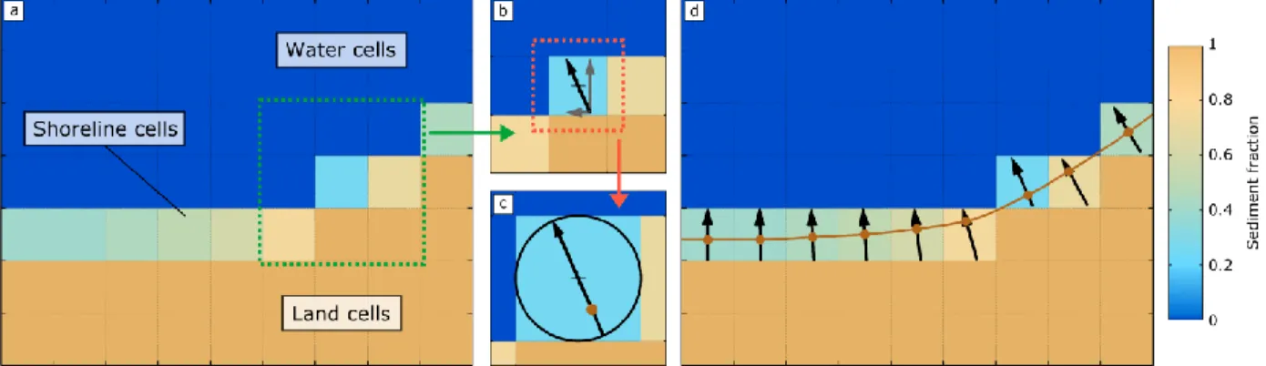
The local shoreline position and orientation are critical to the model as they control the breaking wave parameters and sediment fluxes at each time step, which requires the development of a specific method. First, for each shoreline cell the local shoreline orientation is determined by its cell-based shore normal vector (black arrows in Fig. 5b-d) which is estimated according to the row-wise and column-wise gradients calculated over a 3-by-3-cell sub-grid (green dotted square in Fig.5a) centered on the cell (red dotted square in Fig. 5b). Second, within the shoreline cell, it is assumed that the shoreline crosses the cell-based shore normal vector, which must be previously normalized to the cell size and centered, at a distance from the center of the cell that depends on the sediment fraction value (Fig. 5c). The distance is defined as l = (Fij -
13
0.5) dxy where Fij is the sediment fraction of the shoreline cell. With this definition it is assumed that the
shoreline crosses the cell exactly at its center for Fij = 0.5, while it intercepts the base and the tip of the
cell-based shore normal vector for Fij = 0 and Fij = 1, respectively. Applying this method to every shoreline cell
provides estimates of a realistic shoreline position inside each shoreline cell (hereafter referred to as the cell-based shoreline position, Fig. 5d). This method offers several benefits, e.g. (1) the numerical implementation is simple and robust, (2) it handles all shoreline configurations as long as one neighboring shoreline cell exists and (3) it is computationally cheap as it is based on trigonometry only.
Figure 5. a Example of a sediment fraction (F) grid. b Computation of the shore normal vector (black arrow) giving the shoreline orientation. The vector components (grey arrows) correspond to the column-wise and row-wise gradients in F, computed over the 3-by-3-cell sub-grid denoted by the green contour in a. c Estimate of the shoreline
position (brown dot) inside the shoreline cell surrounded by the red contour in b. d Computation of the complete shoreline (brown curve) by interpolation of all the estimates of shoreline position.
3.3. Waves and bathymetry
Computation of the longshore and cross-shore sediment transport requires knowledge of the breaking wave parameters such as the significant wave height Hs, the mean period Tm (or the peak period Tp) and the mean
wave direction Dm. To ensure flexibility of the model depending on the application, we not only
implemented a basic wave model (option 1), but also coupled the shoreline model with the nearshore spectral wave model SWAN (option 2).
Option 1 relies on the formula of Larson et al. (2010), which is a simplified solution of the wave energy flux conservation equation combined with Snell’s law. This approach has been combined with a shadowing procedure as described in Ashton and Murray (2006a), such that in areas protected from waves (shadowed area), no sediment is transported between cells, and thus no wave computations are required. Option 2 uses the SWAN model (Booij et al., 1999; Ris et al., 1999). First, it should be recalled that the coupling between
14
shoreline changes and waves lies in the evolution of the bathymetry associated to the shoreline changes. Thus, a preliminary step within the coupling is to estimate, at each time step, the bathymetry (h) associated with the shoreline (see Fig. 3 and below for a technical implementation description). Then, the SWAN model uses its own computation grid (hereafter referred to as the hydrodynamic grid), which should be fine enough to ensure that the cross-shore surf zone is described with at least 2-3 cells for morphogenic conditions, i.e. with 10 to 20 m grid cells (Fig 6a,d). SWAN provides gridded outputs for Hs, Tm and Dm,
which are further used to locate and extract the breaking quantities. The default processes and parameters of SWAN are used, except the breaking which is switched off to detect the breaking line based on where the breaker index γ = Hs/h (h being the water depth) becomes lower than the critical value γb. This strategy
is commonly used (see e.g. Limber et al. 2017).
Similarly to the shoreline model of Kaergaard and Fredsoe (2013a), a bathymetry reconstruction module was implemented that updates the bathymetry at each time step according to the new shoreline shape (Fig. 3 and Fig. 6). The water depths (h) are retrieved by projecting the shoreline over the hydrodynamic grid and propagating offshore a constant beach profile (Fig. 6b). LX-Shore uses a beach profile that follows the power law h = α dSL β (as for the equilibrium profile defined by Dean, 1991) where dSL is the shortest distance
from a grid point to the shoreline. The α and β parameters define the beach profile shape and are provided as LX-Shore inputs. To handle the presence of non-erodible areas, a second bathymetry is implemented with the same method but using an additional profile propagated from the non-erodible contours (hereafter referred to as rocky contours, Fig. 6c). The shape of this rocky profile also follows a power law, whose coefficients are also provided as LX-Shore inputs, that allows representing the bathymetry near rocky contours with a concave, convex or linear profile shape. In both cases, when the computed water depth is larger than a critical value (hc), the water depth is set up constant (equal to hc). Finally, the two bathymetries
are merged into a single one (Fig. 6d) by applying the following conditions: (1) at each hydrodynamic grid point the rocky-contour-derived depth hRC does not contribute to the final bathymetry if it is larger (i.e.
deeper) than the shoreline-derived depth hSL (i.e.: h = hSL if hRC ≥ hSL); (2) if not, a weighted average between
the two depths is calculated, the weighting factor a being proportional to the depth difference normalized by the shoreline-derived depth (h = a hRC + (1-a) hSL if hRC < hSL, with a = (hSL - hRC) / hSL). Far from hard
structures, the bathymetric contours are parallel to the shoreline and undulations in the bathymetric contours are smoothed seaward, while getting closer to hard structures, the bathymetric contours become progressively parallel to the rocky contours. The weighted average prevents from having abrupt bathymetric changes when passing from bathymetric contours parallel to the shoreline to those parallel to the rocky-contours. This bathymetry reconstruction method enables SWAN to simulate the modifications of wave
15
fields reaching undulating coasts that include simple geological features (headlands, offshore islands) and artificial structures (groins, breakwaters).
Figure 6. Procedure for the bathymetric computation for the SWAN hydrodynamic grid. a Sediment fraction grid over which the corresponding shoreline (brown line) and the rocky contours (black areas) are projected. b
Shoreline-derived bathymetry, and the corresponding assumed beach profile (α = 0.25, β = 0.67 ). c Rocky-contour-Shoreline-derived bathymetry, and the corresponding assumed rocky profile (α = 0.1, β = 1 ). d Final bathymetry obtained by merging
16 3.4. Longshore transport
The volumetric longshore transport is estimated using either the CERC (USACE, 1984) or the Kamphuis (1991) formulas which read, respectively:
2.5 , sin(2 ) 16( )(1 ) b s b l b s K g H Q p
(6) 2 1.5 0.75 0.25 , 50 0.62.27
sin (2 )
(
)(1
)
s b p b l b sH T m
d
Q
p
(7)where Hs,b is the significant wave height at breaking, θb is the breaking wave incidence angle, Tp is the peak
period, ρs and ρ are the sediment and water density, respectively, p is the sediment porosity, γb is the breaker
index, mb is the beach slope, d50 is the mean sediment grain size, and K is an empirical site-specific
coefficient typically ranging from 0.2 to 1.6 (Arriaga et al., 2017; Bayram et al., 2007; Komar, 1998; Pilkey and Cooper, 2002). Contrary to the CERC formula, the Kamphuis (1991) formula does not require the calibration of K. In addition, the Kamphuis (1991) formula integrates more physics via the dependence on other beach characteristics (mb and d50) as well as Tp. The CERC formula is implemented in LX-Shore
primarily for the sake of model skill comparison with the CEM model (Ashton and Murray 2006a), which is based on the CERC formula. For other applications and in absence of a dataset to calibrate accurately K, the use of the Kamphuis (1991) formula is preferred. Inter-comparisons of these formulas are available in Bayram et al, (2007), Bertin et al. (2008) and Wang et al. (2002).
The longshore sediment transport is estimated at each boundary between two adjacent shoreline cells (Fig. 2). The knowledge of the local shoreline orientation is required to compute the breaking wave parameters used in the longshore transport formula (Hs,b and θb). With option 1 for waves, the local shoreline orientation
allows expressing the input offshore wave direction in terms of offshore wave incidence angle (θ0) that is
used in the Larson et al. (2010) formula. With option 2, the breaking wave parameters are extracted from the SWAN gridded outputs, using an extraction ray that scans the outputs seaward from the shoreline cell boundary, following the direction perpendicular to the local shoreline orientation, in order to locate the breaking point. The local shoreline orientation is also used to express the extracted breaking wave direction in terms of θb (in Fig. 7a). This shoreline orientation is given by the so-called boundary-based shore normal
17
the first axis e1 is parallel to the alignment of the two adjacent shoreline cells and the second axis e2 points
toward the water domain. The e1-component of the vector (ne1) is set equal to the difference in sediment
fraction between the two adjacent shoreline cells while the e2-component (ne2) is always set to one. The
boundary-based shore normal vector is then expressed in the model coordinate system by applying trigonometry transformations. In addition, with option 2 the exact shoreline position at the boundary between the two adjacent shoreline cells is required to set the starting point of the extraction ray. This shoreline position (referred to as the boundary-based shoreline position) is located at the center (red circles in Fig. 7) of the shoreline section comprised between the two adjacent cell-based shoreline positions (brown dots in Fig. 7). Note that the boundary-based shoreline position is not necessarily on an edge or a node of a cell.
Figure 7. a Schematic of the computation of the breaking wave angle of incidence θb (with option 2 for the waves)
defined as the angle between the breaking wave direction vector 𝑤⃗⃗⃗⃗⃗ (white arrows) and the boundary-based shore 𝑏
normal vector 𝑛⃗ (orange arrows). b Schematic of the computation of the boundary-based shore normal vector 𝑛⃗ (orange arrows). ne1 is equal to the shoreline cell sediment fraction difference. ne2 is set to one. The orthogonal basis
(e1, e2) is oriented so that the axis e1 is parallel to the shoreline cell alignment (dotted lines linking the cell centers)
and e2 points in the offshore direction. The brown curve, the brown dots and the red circles represent the interpolated
shoreline, the cell-based shoreline positions and the boundary-based shoreline positions, respectively.
18
The cross-shore sediment transport is calculated using an adaptation of the empirical equilibrium-based ShoreFor model described in Splinter et al. (2014). The ShoreFor model assumes that cross-shore shoreline displacement at a given time depends on both the magnitude of forcing available to move the sand and the disequilibrium between the instantaneous dimensionless fall velocity at breaking (Ωb) and the equilibrium
dimensionless fall velocity (Ωeq) defined as:
eq b
(7)The dimensionless fall velocity reads:
, s b b p
H
wT
(8)where w is the settling velocity. The site-specific equilibrium dimensionless fall velocity is computed using a weighted integration of the past dimensionless fall velocity over a site-specific period (Φ), referred to as beach memory, which can vary from days to years (Davidson et al., 2013; Splinter et al., 2014). The shoreline change rate is finally expressed as:
/ 0.5 c
S
c
P
b
t
(9)where P is the wave energy flux at breaking, σΔΩ the standard deviation of ΔΩ (used to normalize ΔΩ), b a
term added to encapsulate long-term processes not included in the ShoreFor model (e.g. local sediment input or loss). The coefficient c+/- is either equal to c or cr if ΔΩ > 0 or ΔΩ < 0, respectively, where c is a
site-specific rate parameter and r is the erosion ratio. The coefficients Φ, c and b are the model free parameters and are obtained by an optimization procedure against shoreline measurements. In LX-Shore, an adjustment of Eq. (7) has been done. Indeed, computing ΔΩ at breaking requires recording one time series of past breaking wave conditions per shoreline cell (which is memory and time consuming), while computing ΔΩ would be a complex process when new shoreline cells are created (land or water cells becoming shoreline cells) during the simulation. Thus, in order to keep computation time low and avoid issues related with the creation of new shoreline cells during the simulation, a unique time series of ΔΩ is computed in LX-Shore using the offshore wave data. In contrast, P is still calculated using the breaking wave conditions associated with each shoreline cell. Thus, the direction of the shoreline displacement essentially depends on the
19
offshore wave conditions, while the magnitude also depends on local breaking conditions. When option 2 is used to propagate the waves (SWAN), the breaking wave parameters used to compute P are the breaking quantities found offshore the cell-based shoreline positions, following the direction given by the cell-based shore normal vectors.
3.6. Numerical stability, spatial resolution and time step
Similar to hydrodynamic and morphodynamic numerical models that use a CFL condition to determine the maximum time step, the simulation time step in LX-Shore has to be set according to the spatial resolution of the morphological grid and maximum sediment flux to ensure numerical stability in the simulations. Based on the average incident wave conditions, the morphological grid cell size in LX-Shore typically ranges from approximately 10 m for low-energy wave climate to 100 m for high-energy wave climate. Previous tests show that the simulations are stable if the total sediment fraction variation in the shoreline cells during one time step is smaller than 0.5. In cases where only the longshore processes are included in the simulation, the time step has to respect a condition deduced from Eq. (4), which reads Δt ≤ 0.5 dxy2 (D
c
/ Ql,max), where Ql,max is the maximum longshore sediment transport expectable during a model iteration. In
the case where only the cross-shore processes are included, the time step has to be small enough to ensure the respect of a condition deduced from Eq. (5), which reads Δt ≤ 0.5 dxy / (ΔSc /Δt)max, where (ΔSc /Δt)max
is the maximum simulated shoreline change rate owing to cross-shore processes. A first estimate of Ql,max
can be calculated using the time series of offshore wave conditions and shoreline orientation maximizing the longshore sediment transport, while a rough estimate of (ΔSc /Δt)max can be made by analyzing the time
series of measured shoreline position used for the model free parameter calibration. In the case where both longshore and cross-shore processes are included there is no a priori knowledge of their respective contributions. Therefore, it is recommended to respect the two stability conditions above, where a 0.25-threshold can be used instead of 0.5.
4. Synthetic Cases
This section aims at providing an overview of the range of applications of LX-Shore rather than applying the model to a given complex field test case with detailed calibration and model skill assessment. For this purpose, the model is tested with three types of synthetic cases (see simulation set-up in Table 1). The simulations presented here are then briefly discussed and qualitatively compared with observations and/or with results from comparable simulation studies.
The longshore-transport only cases (L) show that the model can simulate the formation and subsequent nonlinear evolution of shoreline instabilities and erosion/accretion pattern downdrift/updrift of coastal structures. The cross-shore-transport only cases (C) show that the model can accurately hindcast shoreline
20
variability on timescales from hours to years at a cross-shore-transport dominated site. Finally, the last test cases (LC) involve both the cross-shore and longshore transport modes. These simulations show the potential to further understand the respective contributions of the cross-shore and longshore transport to address the shoreline temporal and spatial variability on a wide range of sandy coasts and space-time scales.
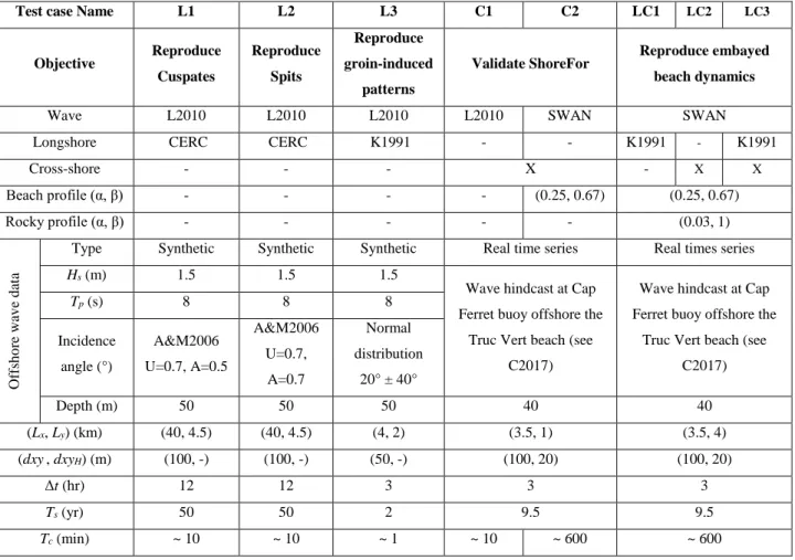
Table 1. Summary of the model set-up of the test cases with K1991: Kamphuis (1991); A&M2006: Ashton and Murray (2006a); L2010: Larson et al. (2010); C2017: Castelle et al. (2017). Lx and Ly are the physical domain size,
dxyand dxyH are the cell size of the sediment fraction grid and the hydrodynamic grid, respectively. Ts and Tc are the
simulated time span (in years) and computation time (in minutes), respectively. SWAN is run on 12 cores.
Test case Name L1 L2 L3 C1 C2 LC1 LC2 LC3
Objective Reproduce Cuspates Reproduce Spits Reproduce groin-induced patterns
Validate ShoreFor Reproduce embayed
beach dynamics
Wave L2010 L2010 L2010 L2010 SWAN SWAN
Longshore CERC CERC K1991 - - K1991 - K1991
Cross-shore - - - X - X X Beach profile (α, β) - - - - (0.25, 0.67) (0.25, 0.67) Rocky profile (α, β) - - - (0.03, 1) Offs h o re wa v e d ata
Type Synthetic Synthetic Synthetic Real time series Real times series
Hs (m) 1.5 1.5 1.5
Wave hindcast at Cap Ferret buoy offshore the
Truc Vert beach (see C2017)
Wave hindcast at Cap Ferret buoy offshore the
Truc Vert beach (see C2017) Tp (s) 8 8 8 Incidence angle (°) A&M2006 U=0.7, A=0.5 A&M2006 U=0.7, A=0.7 Normal distribution 20° ± 40° Depth (m) 50 50 50 40 40 (Lx, Ly) (km) (40, 4.5) (40, 4.5) (4, 2) (3.5, 1) (3.5, 4) (dxy, dxyH) (m) (100, -) (100, -) (50, -) (100, 20) (100, 20) Δt (hr) 12 12 3 3 3 Ts (yr) 50 50 2 9.5 9.5 Tc (min) ~ 10 ~ 10 ~ 1 ~ 10 ~ 600 ~ 600
For the simulations using SWAN for wave propagation (option 2), the beach and rocky profile coefficients are required to compute the bathymetry. The best-fit beach profile coefficients (shown in Table 1) obtained from a comparison with the longshore- and time-averaged profiles at Narrabeen beach (using the bathymetric dataset available from Turner et al., 2016) are used. The rocky profile is assumed linear (β = 1) and its slope is set steeper than the overall beach profile slope (Table 1) so that the rocky contours contribute to the final bathymetry only in the close vicinity of the rocky features (Fig. 6). For application to real sites,
21
the rocky profile shape (curvature and steepness), which is set arbitrarily here, should be designed based on the field site characteristics. For simulations involving longshore transport, Dc is set arbitrarily to 10 m as
in Ashton and Murray (2006a) as it belongs to the range of closure depth for wave-dominated coastlines (Arriaga et al., 2017; Kaergaard and Fredsoe, 2013c; Ratliff and Murray, 2014; Ruggiero et al., 2010) and because the model is applied to synthetic cases only.
4.1. Longshore only
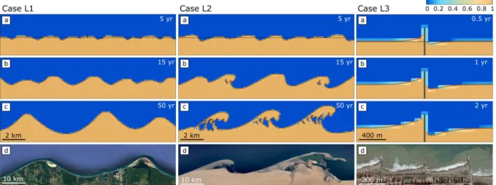
In test cases L1, L2 and L3 (Table 1), only the longshore transport is turned on, while wave characteristics at breaking are computed using the Larson et al. (2010) formula. First, we focus on the model skill to reproduce self-organized patterns such as large cuspates (L1) and flying and reconnecting spits (L2). Similarly to reference studies aiming at reproducing such morphological features (Ashton et al., 2001; Ashton and Murray, 2006a, 2006b), the CERC formula is used for these two test cases with the same calibration coefficient as in Ashton and Murray (2006a) (K = 0.85). Simulations (L1a-c and L2a-c in Fig. 8) start from a straight shoreline exposed to idealized wave climates characterized by a constant wave height and period (Hs = 1.5 m and Tp = 8 s) but time-varying wave direction. Following the method of Ashton and
Murray (2006a), the wave direction time series is computed by randomly selecting values from a probability distribution function of wave direction defined by the asymmetry and the highness parameters (A and U respectively). The parameter A ranging from 0 to 1 defines the proportion of waves coming from the left, meaning that for A = 0 (A = 1) all the waves come from the right (left) while for A = 0.5 there is as much wave influence coming from the left as from the right. The parameter U ranges from 0 to 1, and defines the proportion of waves having an offshore wave incidence angle greater than 45°. For U = 0 (U = 1) all the waves are low angle (high angle) while for U = 0.5 the probability of having offshore high and low incidence wave angle is the same. The initial shoreline is perturbed by adding white noise, the maximal noise amplitude being equal to the morphological grid cell size. The simulation is performed over a 50-year period. The first test case (L1) is conducted with a symmetrical wave climate (A = 0.5) and a large proportion of high-angle waves (U = 0.7). The second test case (L2) is the same but with an asymmetrical wave climate (A = 0.7). For both simulations the shoreline is unstable with shoreline rhythms rapidly developing with short and irregular wavelengths. The shoreline instabilities subsequently self-organize into more alongshore-uniform features and increase in wavelength through feature merging. In agreement with the findings of Ashton and Murray (2006a, 2006b), the symmetrical wave climate leads to the development of large cuspate bumps (Fig. 8L1a-c), while the asymmetrical wave climate leads to the formation of spits which sometimes reconnect to the beach (Fig. 8L2a-c). The latter simulation demonstrates the robust numerical implementation of the model to handle the dynamics of complex shoreline plan-view shapes,
22
including trapped water bodies and propagating spits. In terms of computation time, the model enables simulating 50 years in 10 minutes.
Using the CEM model with a wave climate defined by Hs = 2 m, T = 8 s, A = 0.5 and U = 0.7 Ashton and
Murray (2006a) simulated the development of cuspates with a mean wavelength and aspect ratio (amplitude to wavelength) of approximately 9 km and 0.12, respectively, after 50 years of simulation. Here, mean wavelength and aspect ratio of approximately 5.1 km and 0.25, respectively, are obtained with LX-shore after the same simulation period. Performing the same simulation with the wave climate of Ashton and Murray (2006a), i.e. changing Hs = 1.5 m to Hs = 2 m, results in a mean wavelength and aspect ratio of
approximately 8.9 km and 0.3, respectively. Therefore, LX-Shore simulates the development of cuspates with similar wavelengths as with CEM, but with larger offshore expansion. In CEM, the shoreface is assumed to translate over a sloping shelf, imposing an increase in the active profile depth as the shoreline progrades seaward and, in turn, a progressive saturation of the amplitude of the shoreline instabilities. This mechanism is not included in LX-Shore, which explains why the obtained aspect ratios are larger. LX-Shore does not include an overwash algorithm as in CEM, which prevents sand spits from breaching at their base in their simulations where such shoreline patterns emerged. This algorithm is shown to significantly change the shape of the simulated sand spits (Ashton and Murray, 2006a) as without breaching the longshore transport directed to the tip of sand spits is never interrupted, which, in turn, allows sand spits to continuously prograde seaward. This likely explains the smaller offshore extensions of the sand spits simulated with LX-Shore, which frequently breach at their base. The quantitative assessment of model skill to simulate such shoreline instabilities is out of the scope of this study.
Figure 8. Results of test cases L1, L2, L3 (longshore transport only, see Table 1) and field examples. a-c Simulated shoreline position (brown line). The initial shoreline is indicated by the black dotted line (row a). d: Natural
23
examples of (L1d) cuspate shoreline (Ludington and Penwater beaches, Lake Michigan, USA), (L2d) flying/reconnecting sand spits (Walvis Bay nearby coast, Namibia), (L3d) erosion and accretion resulting from a groin trapping the longshore drift (Moncofa beach, Spain). Source: Google Earth imagery. The longshore and
cross-shore scaling are the same in each sub-figure.
Second, LX-Shore is used to simulate shoreline evolution after the implementation of a 20-m wide groin extending 200 m offshore disrupting the longshore drift along an initially straight sandy coast. The wave height and period are constant (Hs = 1.5 m and Tp = 8 s) while the wave direction is time-varying (see Table
1), with a modal direction corresponding to an offshore wave incidence angle of 20° (coming from the left). The results (Fig. 8L3a-c) show that the model is able to reproduce the accretion and erosion patterns occurring updrift and downdrift of the groin, respectively. After 2 years, the simulated maximal accretion is about 125 m on the left (updrift) side of the groin while maximal erosion is about 100 m on the right (downdrift) side. In this case, the computation time is about 1 minute. Overall, these test cases show that the LX-Shore model is able to reproduce both free (self-organized) and forced (hard structures) shoreline dynamics controlled by alongshore processes with low computational cost.
4.2. Cross-shore only
In the test cases C1 and C2 (Table 1), only the cross-shore transport is switched on, while the breaking wave parameters are calculated using the Larson et al. (2010) formula and the SWAN model, respectively. The selected site for validation is Truc Vert beach, located on the French Atlantic coast (see Castelle et al., 2017 for an extensive field site description), where the gradients in longshore drift are negligible (Idier et al., 2013). The model set-up consists of a 1-km-long straight beach. The simulations are performed over the 9-year period of shoreline measurements. The time series of offshore wave height and incidence angle are shown in Figure 9a,b.
The free parameters Φ, c and b are determined by optimization of the cross-shore model with real shoreline measurements while the r coefficient is calculated from the time series of breaking waves. To reduce the number of unknown of the system, Φ is set to 900 days based on the findings of Splinter et al. (2014) and Castelle et al. (2014). It is well established that Truc Vert is a high-energy intermediate sandy beach responding predominantly at the seasonal time scale (Castelle et al., 2014; Splinter et al., 2014), that is, with a beach memory Φ typically longer than 500 days (simulations with Φ = 500, 1000 or 2000 days give similar results). In order to speed up the calibration process, Φ is set to 900 days. The first step consists of extracting the breaking wave parameters time series along a cross-shore transect. To do so, the model is run over the simulation period turning off the sediment transport. The comparison between the C1 and C2 results shows
24
that the computed breaking wave conditions are very similar for both test cases (not shown). The time series of wave breaking parameters being computed, the r coefficient is calculated following Splinter et al. (2014). Finally, the two last model parameters (c and b) are determined by minimizing the root-mean-square error (RMSE) between concurrent model predictions and measurements of shoreline position using the Simulated Annealing algorithm (Bertsimas and Tsitsiklis, 1993) as in Castelle et al. (2014). The calculated values for
r, c and b are presented in Table 2, showing similar values in the two test cases and, as a result, very similar
shoreline evolutions (Fig. 9c). The comparison with measured shoreline position (grey dots in Fig. 9c) shows that the model successfully simulates shoreline variability on timescales from hours to years through seasons. For instance, the winter-storm-driven erosion events during the winter 2013-2014 (Castelle et al. 2015) is captured, which was identified as the most energetic winter along the Atlantic coast of Europe for the last 50 years (Masselink et al., 2016b, 2016a). Over the entire simulation period, the determination coefficients are 0.67 and 0.65, and the RMSE are 7.74 m and 7.58 m, for test cases C1 and C2 respectively. The same skills are obtained by Castelle et al. (2014) and Splinter et al. (2014) when applying the original version of the ShoreFor model to the Truc Vert beach. Finally, these test cases highlight the cost of using SWAN instead of Larson et al. (2010): the computation time is 60 times longer when using the SWAN model (Table 1) on a 12 core CPU. Using Larson et al. (2010) as the LX-Shore wave driver is therefore relevant for reasonably simple shoreline plan-view shapes.
25
Figure 9. a-b: Time series of offshore wave height and incidence angle used in test cases C1,C2, LC1, LC2 and LC3. The thick red line indicates the 90-day moving average. c Results of test cases C1 and C2: time series of cross-shore shoreline position measured (grey dots), simulated using the Larson et al. (2010) formula (test case C1, red line) and
simulated using SWAN (test case C2, black line).
Table 2. Cross-shore model coefficients obtained for test cases C1 and C2, with Φ set to 900 days. Test Case Computing method for breaking waves r c (m1.5.s-1.W-0.5) b (m.yr-1)
C1 Larson et al. (2010) 0.221 5.68∙10-8 -2.89
C2 SWAN 0.210 5.92∙10-8 -2.90
4.3. Embayed beach
The last type of test cases addresses the shoreline dynamics along an idealized embayed beach where cross-shore and alongcross-shore processes co-exist and where wave refraction and shadowing from headlands affect breaking wave conditions (LC1, LC2, LC3, Table 1). Three test cases are conducted: longshore only (LC1), cross-shore only (LC2), and cross-shore and longshore (LC3). The model is applied to a 3.5-km-long straight beach bordered by two rectangular headlands extending approximately 400 m offshore (Fig. 10a). The beach is exposed to the same wave climate as the simulations described in subsection 4.2 (Fig. 9a-b). SWAN model is used to obtain the wave conditions at breaking. The calibration coefficients of test case C2 are used for cases LC2 and LC3 (where the cross-shore model is turned on).
Results of test case LC1 are depicted in Figure 10b and Figure 10e that show the timestack of the shoreline position, with the corresponding time series at three representative locations within the embayment. From the beginning of the simulation in 2005 until the winter 2009-2010, a 2.3° clockwise shoreline rotation occurs, followed by a relatively stable 2-year period and a subsequent new increase of the rotation signal between the winter 2011-2012 and the winter 2013-2014. Throughout the simulation, the shoreline progressively becomes curvilinear (light grey line in Fig. 10a) which is consistent with the typical shape of embayed beaches (Fig. 1b). After 9 years of simulation, the curvature is quite low. This is in line with Hurst et al. (2015) who found that the curvature of crenulated beaches remains very low for wave climates having a dominant wave incidence angle lower than 15°.
With cross-shore transport only (LC2 test case), the shoreline essentially moves uniformly offshore or onshore in response to changes in incoming wave energy (Fig. 10c,f), except close to the headlands as a result of wave shadowing. In addition to the short timescale variability, the cross-shore-transport also drives slight long-term shoreline erosion that is not present in the results obtained in test case LC1. Taking into
26
account both longshore and cross-shore transport (LC3, Fig. 10d,g) leads to a modulation of the beach rotation signal at storm-event and seasonal timescales. The final beach plan-view shape (black line in Fig. 10a) is curvilinear, as in test case LC1, but slightly more eroded. This is due to the slight long-term shoreline erosion induced by the cross-shore transport (test case LC2). It should be noted that the shoreline evolution induced by both longshore and cross-shore transport is slightly different to the sum of the shoreline evolutions induced by each transport simulated in isolation. Indeed, as the coast rotates due to alongshore processes, the shoreline orientation becomes more perpendicular to the mean wave direction, wave refraction is reduced and wave conditions at breaking are slightly different from the breaking wave conditions obtained when the shoreline evolution is spatially uniform (i.e. when only the cross-shore transport is taken into account).
Figure 10. Results of test cases LC1, LC2, LC3. a Model geometry: straight shoreline bordered by two 400-m long headlands. Brown, light grey, grey and black line show the initial shoreline and the final shoreline for test cases LC1,
27
LC2 and LC3, respectively. b-d Timestacks of cross-shore shoreline position enabling the longshore transport only (LC1), the cross-shore transport only (LC2) and both (LC3), respectively. e-g Time series of cross-shore shoreline position at the alongshore positions indicated by the vertical lines in panels b-d. Y0 corresponds to the initial
cross-shore position of the cross-shoreline.
5. Discussion
5.1. Current assumptions and limitations
This new shoreline change model is based on several assumptions that are here reminded and discussed, allowing an assessment of the application range at the current stage of LX-Shore development. Shoreline changes are assumed to be controlled only by wave-driven sediment transport occurring over the active and sediment rich shoreface (the shoaling and surf zones). LX-Shore accounts for sediment transport resulting from both alongshore and cross-shore processes to allow investigating shoreline change on a wide range of beaches and temporal scales. Overwash effects are however neglected at this time, preventing model application to gentle-slope beaches backed by low-elevation dunes, such as barrier islands, where overwash can dominate short- (Lindemer et al., 2010; Matias et al., 2016; McCall et al., 2010) to long-term (Jiménez and Sánchez-Arcilla, 2004; Leatherman, 1979; Lorenzo-Trueba and Ashton, 2014) coastal change. LX-Shore still remains applicable to a wealth of sites, as high dunes and/or rocky cliffs backing beaches are common features worldwide. In the model, rocky areas are non-erodible and influence shoreline change through obstruction of longshore sediment transport (Ratliff and Murray, 2014) and deformation of the incident wave field resulting from shadowing, refraction and diffraction effects. However, for sandy coasts that include a large proportion of rocky areas exposed constantly or even intermittently to waves, weathering of these areas represents a source of sediments, and beach-cliff interactions can contribute to the long-term coastal dynamics (Limber and Murray, 2011; Valvo et al., 2006). The model neglects the effect of the sea-level rise, which also contributes to shoreline change in the long-term through passive flooding and/or onshore translation of an equilibrium shoreface shape (Bruun, 1962), although for the latter the basic assumption is still subject to debate (Cooper and Pilkey, 2004; Ranasinghe et al., 2012). Finally, addressing the influence of estuaries and tidal inlets is challenging. It is well established that maximum shoreline evolutions are often observed along coasts adjacent to the inlets and to the estuary mouth, with erosion and accretion alternating on timescales of decades (e.g. Castelle et al., 2018). These long-term changes are more or less linked to auto-cyclic variability of the tidal environment and riverine hydraulics, which cannot be addressed without using a fully coupled hydrodynamic-based model that would dramatically increase the computational cost. Accordingly, LX-Shore must be applied on coasts away from the influence of tidal inlets and estuary mouths.
28
The model is fundamentally based on the one-line concept and thereby assumes the beach profile remains unchanged and only translates as the cross-shore shoreline position evolves. While the magnitude of shoreline change in response to longshore gradients in sediment transport depends on Dc, the magnitude of
shoreline change driven by cross-shore processes is independent from beach profile geometry and essentially depends on present and past wave forcing. Addressing large-scale coastal change on timescales greater than decades or a century requires using large Dc of ~ 20-50 m (Kaergaard and Fredsoe, 2013a,
2013c; Ortiz and Ashton, 2016; van den Berg et al., 2012). On the timescales at which cross-shore processes are resolved in LX-Shore, i.e. up to years and likely some decades pending a long calibration period, profile perturbation in the surf zone or in the upper shoreface are no longer assumed to propagate that far offshore within the lower shoreface. Using large Dc when including cross-shore processes leads to underestimate
shoreline change driven by longshore gradients in longshore sediment transport as deposited or eroded sediment volumes are distributed deeper than for cross-shore processes. Thus, the choice in Dc is crucial to
avoid such mismatch in the timescales and to compare the respective contributions of alongshore and cross-shore processes. On timescales from a year to decades, shallower Dc of ~ 5-20 m must be used (Hanson,
1989; Kaergaard and Fredsoe, 2013c; Ruggiero et al., 2010; Szmytkiewicz et al., 2000; van den Berg et al., 2012). The use of the theoretical framework developed by Ortiz and Ashton (2016) provides an objective method to determine Dc according to the timescales of interest.
In LX-Shore, an idealized bathymetry is reconstructed when the waves are propagated with SWAN (option 2). At this stage of development, this bathymetry is obtained using an empirical method that propagates seaward an equilibrium beach profile from the shoreline and a simple, idealized rocky profile from rocky-contours. Although this method allows computing rapidly a bathymetry for any coastline geometry, it cannot include offshore bathymetric singularities (e.g. submerged rocky outcrops) or spatially-varying rocky profile shapes that both affect offshore wave propagation and/or depth-induced breaking. Similar to the majority of the other shoreline models, LX-Shore assumes a constant shape of the active shoreface (here, a beach profile with constant shape coefficients). However, as a result of substantial change in wave exposure and on long timescales (years), the beach state can change from a more dissipative to reflective state and vice versa, i.e. with a temporal variation of shape of the shoreface profile. Thus, in its present version, LX-Shore should be used with caution at sites where such beach state changes are expected.
Short-term morphological variations (e.g. changes caused by surf zone sandbar dynamics) are regarded as negligible perturbations superimposed on the main trend of shoreline evolution, which is one of the underlying assumptions of the use of an idealized beach profile. In the case of the meso-macro-tidal straight