ScienceDirect
Comput. Methods Appl. Mech. Engrg. 321 (2017) 294–315
www.elsevier.com/locate/cma
A–
φ formulation of a mathematical model for the induction
hardening process with a nonlinear law for the magnetic field
Jaroslav Chovan
a, Christophe Geuzaine
b, Marián Slodiˇcka
a,∗aDepartment of Mathematical Analysis, Ghent University, Ghent, Belgium
bDepartment of Electrical Engineering and Computer Science, Montefiore Institute, University of Liege, Liege, Belgium
Received 28 October 2016; received in revised form 2 March 2017; accepted 30 March 2017 Available online 25 April 2017
Abstract
We derive and analyze a mathematical model for induction hardening. We assume a nonlinear relation between the magnetic field and the magnetic induction field. For the electromagnetic part, we use the vector–scalar potential formulation.
The coupling between the electromagnetic and the thermal part is provided through the temperature-dependent electric conductivity and the joule heating term, the most crucial element, considering the mathematical analysis of the model. It acts as a source of heat in the thermal part and leads to the increase in temperature. Therefore, in order to be able to control it, we apply a truncation function.
Using Rothe’s method, we prove the existence of a global solution to the whole system. The nonlinearity in the electromagnetic part is handled by the theory of monotone operators. To supplement our theoretical results we provide a numerical simulation using real physical constants.
c
⃝2017 Elsevier B.V. All rights reserved.
MSC 2010:35K61; 35Q61; 35Q79; 65M12
Keywords:Maxwell’s equations; Minty–Browder; Monotone operators; Rothe’s method; Scalar potential; Vector potential
1. Introduction
There are many papers dealing with mathematical models of the induction hardening process. Some of them
provide various numerical schemes e.g. [1–6]. But they omit mathematical or numerical analysis of their models
and numerical schemes. Other papers deal with the well-posedness of the problem and provide theoretical results
e.g. [7–11]. The topic of induction hardening has been broadly covered in papers [12,13] and [14]. However, all
manuscripts tackling the theoretical side of the induction hardening phenomena present mathematical models with
linear dependency between magnetic and magnetic induction field. The papers [15,16] studied a mathematical model
∗ Corresponding author.
E-mail addresses:[email protected](J. Chovan),[email protected](C. Geuzaine),[email protected](M. Slodiˇcka). URLs:http://cage.ugent.be/∼jchovan(J. Chovan),http://montefiore.ulg.ac.be/∼geuzaine(C. Geuzaine),http://cage.ugent.be/∼ms(M. Slodiˇcka).
http://dx.doi.org/10.1016/j.cma.2017.03.045
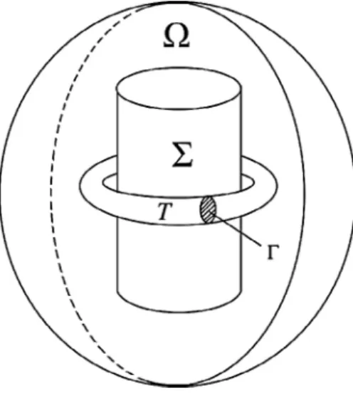
Fig. 1. Illustration of the domain.
with a nonlinear relation between those two vectorial fields (which better reflects the reality), but the study was restricted just to a conductor, i.e. the domain had only one component. The authors proved solvability for a formulation with either magnetic induction or magnetic field as unknown. We present the vector–scalar potential formulation for a nonlinear setting including conducting and non-conducting parts, i.e. the domain consists of multiple components. This means that material coefficients may have jumps across the interfaces. To our best knowledge nothing similar has been done before.
1.1. Derivation of a mathematical model
We work only with a simplified model of induction hardening process (seeFig. 1). The time frame is denoted by
[0, T ]. Let Ω be a bounded sphere in R3. The workpiece and the coil are represented by Σ and T , respectively. Both
Σ and T are closed subsets of Ω and the following holds
Σ ∩ T = ∅, and ∂Σ , ∂T, ∂Ω are of class C1,1. (1)
Conductors are affected by temperature, hence we separate them from the rest of the domain Ω by denotingπ = Σ∪T .
Current in the coil is modeled via an interface condition on Γ . Byν we denote the standard outer normal unit vector
associated with surfaces of materials under consideration.
We start deriving our mathematical model with introducing the classical Maxwell equations (for reference, see [17])
∇ ·D =ρ, (2)
∇ ·B = 0, (3)
∇ ×E = −∂tB, (4)
∇ ×H =∂tD + J. (5)
Here, D stands for displacement current andρ is the density of electrical charge. The magnetic induction field, the
electrical field and the magnetic field are denoted with B, E and H, respectively. At last, J indicates the source current. For the clarity, we note that equations above are true in the whole domain Ω .
In models dealing with eddy currents, the time variation of displacement current is insignificant, therefore we neglect it. We present the nonlinear relation between H and B in the following form:
H :=µM(B) = 1
Magnetic permeabilityµ = µ1∗ might behave differently in the workpiece and in the air, therefore, we specify it as a
split function
µ(x) ={µµπ(x), if x ∈ ¯π,
A(x), if x ∈ Ω \ ¯π.
(7)
Bothµπ andµA are strictly positive and bounded. There is no jump in the tangential component of H along the
boundaries between different materials, i.e.
[µM(∇ × A) × ν]∂π =0.
The vectorial field M is supposed to be potential and its potential is denoted ΦM, i.e. ∇ΦM =M, cf. [18]. Moreover,
we assume that M is strictly monotone and Lipschitz continuous. Furthermore, we introduce Ohm’s law
J =σE. (8)
Functionσ represents the electric conductivity and it is defined as follows
σ(u(x, t)) = {
σπ(u(x, t)), if x ∈ π, t ∈ [0, T ],
0, if x ∈ Ω \π, t ∈ [0, T ], (9)
where u(x, t) is a function of temperature in the workpiece and the coil. We consider σ to be continuous, bounded
and strictly positive inπ. Since Ω is a simply-connected domain and(3)is true in the whole Ω , we use ([19, Theorem
3.6]) to obtain exactly one magnetic vector potential A ∈ H(curl ; Ω ) with the following properties:
B = ∇ × A, ∇ ·A = 0, A ×ν = 0 on ∂Ω. (10)
Substituting(10)into(4)we get
∇ ×(E +∂tA) = 0 in Ω. (11)
Using(11), we apply ([19, Theorem 2.9]) to acquire a unique scalar potentialφ ∈ H1(Ω )/R such that:
E +∂tA = −∇φ. (12)
Taking into account the insignificance of∂tD and using(12),(10),(8),(6),(5)we arrive at the following boundary
value problem for vector potential A:
σ ∂tA + ∇ ×µM(∇ × A) + σχT∇φ = 0 for a.e. (x, t) ∈ Ω × (0, T ) := QT,
A ×ν = 0 for a.e. (x, t) ∈ ∂Ω × (0, T ),
A(0) = A0 for x ∈ Ω, t = 0.
(13)
Characteristic functionχT has value 1, if x ∈ T and 0 otherwise. We use it, because the external source of the current,
which is defined by the gradient of the scalar potential, is present only in the coil (T , seeFig. 1).
Combination of(8)and(12)gives us an expression for the total current density J
J = −σ∂tA −σ∇φ.
The impressed part Jsour ce= −σ∇φ is caused by an external source and the induced part Ji nduced = −σ∂tA is caused
by the magnetic induction field B in the coil. Demanding that the continuity equation holds for the source current Jsour ce, i.e.
∇ ·Jsour ce =0
we define the scalar potentialφ by the following elliptic equation with homogeneous Neumann boundary condition
on∂T and interface condition on Γ , cf. [12]:
−∇ ·(σπ∇φ) = 0 for a.e. (x, t) ∈ T × (0, T ), −σπ∂φ ∂ν =0 for a.e. (x, t) ∈ ∂T × (0, T ), [ −σπ∂φ ∂ν ] Γ = j for a.e. (x, t) ∈ Γ × (0, T ). (14)
External source current density is represented by function j (x, t), which is assumed to be Lipschitz continuous in time. Jump across interface Γ is indicated by [·]Γ.
Eddy currents generated in the workpiece raise temperature by a significant amount. This phenomenon is called Joule heat and it is expressed as
J · E(8)=σπ|E|2(12)= σπ⏐⏐∂tA +χT∇φ⏐⏐
2
. (15)
This term is crucial and causes numerous troubles during mathematical treatment (unboundedness). Therefore, we introduce a cut-off function and work with truncated Joule-heating term
Rr(x) := ⎧ ⎨ ⎩ r> 0 if x > r, x if |x| ⩽ r, −r if x < −r. (16)
Evolution of temperature in the workpiece and the coil (π, see Fig. 1) is characterized by the following parabolic
nonlinear equation with the homogeneous Neumann boundary condition:
∂tβ(u) − ∇ · (λ∇u) = Rr(σπ(u)
⏐ ⏐∂tA +χT∇φ⏐⏐ 2) for a.e. (x, t) ∈ π × (0, T ), −λ∂u ∂ν =0 for a.e. (x, t) ∈ ∂π × (0, T ), u(0) = u0 for x ∈π, t = 0. (17)
Continuous functionλ(x, t) is supposed to be strictly positive and bounded. The nonlinear function β is of a linear
growth and its derivative is bounded from below by a positive constant.
Eqs.(13), (14)and (17)model the process of induction hardening in our simplified domain Ω . They are tied
together through terms ∇φ, σ and ∂tA. One could ask, whether the artificial intervention in the form of cut-off
function was correct. In real applications of induction hardening, there is always a switch-off button, which is used to prevent the workpiece from thermal deformations. When the temperature reaches a certain degree, this button is turned-off, the stream of electric current is stopped and the workpiece is cooled down. Therefore, applying the cut-off
function on Joule-heating term in(17), is actually a simulation of this switch-off button and indeed, necessary to be
done.
2. Functional setting 2.1. Variational formulation
Let us start with some basic notations. Through the whole paper we adopt notation (·, ·)Ω for the standard
inner product in L2(Ω ) or L2(Ω ). Norm induced by this inner product is indicated as ∥·∥L2(Ω ). Set of functions
k :[0, T ] → Y equipped with the norm maxt ∈[0,T ]∥·∥Y is denoted as C([0, T ]; Y ). In a case when p > 1, norm in
Lp((0, T ); Y ) is defined as(∫T
0 ∥·∥ p Y dt
)1p
. Set of all functionsφ + c, where φ ∈ H1(T ) and c is a constant is marked
asφc.
Considering the vector potential A, we introduce the Hilbert space
XN,0= {ϕ ∈ H(curl ; Ω); ∇ · ϕ = 0, and ϕ × ν = 0 on ∂Ω},
where H(curl ; Ω ) = {ϕ ∈ L2(Ω ) : ∇ × ϕ ∈ L2(Ω )}. Using Friedrichs’ inequality for vectorial fields (cf.
[19, Lemma 3.4] or [20, Cor. 3.51]) we see that we may furnish XN,0with norm ∥ϕ∥XN,0 := ∥∇ ×ϕ∥L2(Ω ). Taking
into account(1), we use [19, Theorem 3.7] or [21, Theorem 2.12] to conclude that XN,0 is a closed subspace of
H1(Ω ).1 Multiplying(13)by a test functionϕ ∈ XN,0, integrating over Ω and using Green’s theorem, we obtain the
1The relation X
N,0 ⊂H1(Ω ) is crucial for our mathematical approach. We would like to point out that the same inclusion is valid also for
convex domains (with non smooth boundary). In such a case one can rely on the [21, Theorem 2.17]. All presented results hold true also for convex domains.
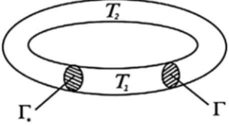
Fig. 2. Dissection of T .
variational formulation for vector potential A:
(σπ∂tA, ϕ)π +(µM(∇ × A), ∇ × ϕ)Ω+(σπ∇φ, ϕ)T =0 ∀ϕ ∈ XN,0. (18)
To obtain the variational formulation for(14), we split T in two separate parts T1 and T2. Flux of the scalar
potential on the new interface Γ∗ is supposed to be continuous. Moreover, Γ∗∩Γ = ∅ and T1∩T2 =Γ∗∪Γ (see
Fig. 2). Now, we multiply(14)by a test functionξ ∈ H1(T )/R and integrate in T
1and T2. Using Green’s theorem,
boundary condition(14)and continuous condition on Γ∗, we arrive to the following variational formulation for scalar
potentialφ:
(σπ∇φ, ∇ξ)T +( j, ξ)Γ =0 ∀ξ ∈ H1(T )/R. (19)
The choice of the test space H1(T )/R is just to obtain a unique solvability.
Lemma 1. There are positive constants c1and c2such that:
c1∥φc∥2H1(T )/R⩽ ∥∇φ∥
2
L2(T )⩽ c2∥φc∥2H1(T )/R.
Proof. Norm in H1(T )/R is defined as ∥φ
c∥H1(T )/R:=infφ∈φc∥φ∥H1(T ). This norm is minimal for c = −|T |1
∫
Tφ dx.
Indeed, let us take a closer look.
0 = d dc (∫ T (φ + c)2+ |∇φ|2dx ) =2 ∫ T φ dx + 2∫ T cdx H⇒ c = − 1 |T | ∫ T φ dx. Now, we write ∥φc∥H1(T )/R= φ− 1 |T | ∫ Tφ dx
H1(T ). Using Poincar´e-Wirtinger inequality, cf. [22] we conclude the
following: ∥φc∥2 H1(T )/R= φ − 1 |T | ∫ T φ dx 2 L2(T ) + ∥∇φ∥2 L2(T )⩽ cP W∥∇φ∥2L2(T )+ ∥∇φ∥ 2 L2(T ) =(cP W+1)∥∇φ∥2L2(T ),
where cP W is a positive constant. Taking c2=1 and c1= 1+c1
P W, the proof is completed. □
For Eq.(17)we follow identical steps as above, using ψ ∈ H1(π) as a test function, which brings us to the
variational formulation for function u:
(∂tβ(u), ψ)π+(λ∇u, ∇ψ)π = ( Rr(σπ ⏐ ⏐∂tA +χT∇φ⏐⏐ 2) , ψ) π ∀ψ ∈ H 1(π). (20) Norm in H1(π) is defined as ∥ψ∥2H1(π):= ∥ψ∥ 2 L2(π)+ ∥∇ψ∥ 2 L2(π).
2.2. Assumptions
To achieve better clarity and readability of our paper, we list all assumptions altogether:
(a1) 0< µπ∗⩽ µπ(x)⩽ µπ∗< ∞ ∀x ∈ Σ,
(a2) 0< µA∗⩽ µA(x)⩽ µ
∗
A < ∞ ∀x ∈ Ω \ Σ,
(b) µ∗=min {µπ∗, µA∗}, µ∗ =max
{ µπ∗, µ∗A } (c1) µ ∈ H1(π) (c2) µ ∈ H1(Ω \π) (d) 0< σ∗⩽ σ (u(x, t)) ⩽ σ∗ < ∞ ∀(x, t) ∈ π × (0, T ), (e1) 0< λ∗⩽ λ(x, t) ⩽ λ∗< ∞ ∀(x, t) ∈ π × (0, T ), (e2) |λ(x, t2) −λ(x, t1)|⩽ Cλ|t2−t1| Cλ> 0, ∀x ∈ π, ∀t2, t1∈[0, T ] (f) | j (x, t2) − j (x, t1)|⩽ Cj|t2−t1| Cj > 0, ∀x ∈ Γ , ∀t2, t1∈[0, T ], (g) j ∈ L2((0, T ); H−1/2(Γ )), ∫ Γ jdΓ = 0, (h) u0∈ H01(π), (i) A0∈xN,0, (j) β is continuous, β(0) = 0, |β(x)| ⩽ Cβ(1 + |x|), 0 < β∗ ⩽ β′(x) Cβ> 0, ∀x ∈ R, (k1) (M(x) − M(y)) · (x − y)⩾ cM|x − y|2 cM> 0, ∀x, y ∈ R3, (k2) |M(x) − M(y)|⩽ CM|x − y| CM > 0, ∀x, y ∈ R3, (k3) M(0) = 0. (21)
Following [18, Theorem 5.1], we see that potential ΦMof vectorial field M with properties (k1)–(k3), is strictly convex.
Applying [18, Theorem 8.4], we get
M(x) · (x − y)⩾ ΦM(x) − ΦM(y) ∀x, y ∈ R3. (22)
Thanks to (k1) and (k2), we bound ΦMfrom below
ΦM(x) = ∫ 1 0 M(x p) · x d p = ∫ 1 0 M(x p) · (x p) p−1d p ⩾ ∫ 1 0 cM|x p|2p−1d p = cM 2 |x| 2. (23) We get ΦM(x)⩽ CM 2 |x| 2 (24)
from (k2) in the same way.
3. Existence of a weak solution
3.1. Time discretization scheme and a priori estimates
In this section we discretize the time interval [0, T ] and solve a system of steady-state differential equations on each time step. Afterwards, we construct piece-wise constant and piece-wise linear in time functions and show convergence of sub-sequences of these functions in appropriate functional spaces to the weak solution. This approach is called
Rothe’s method [23,24]. Consider a number of time steps n ∈ N. We introduce a time discretization of [0, T ] in the
following sense:
[0, T ] = ⋃
0⩽i⩽n−1
[ti, ti −1], where ti =iτ, 0 ⩽ i ⩽ n, nτ = T .
The value of any function f at ti is denoted as fi. To approximate the time derivative of f at ti we use the explicit
Euler method, i.e. ∂tf(ti) :=δ fi=
fi− fi −1
Applying this method to the system(18),(20),(19) we are able to approximate it at every time step ti, for i = 1, . . . , n ( σπ(ui −1)∇φci, ∇ξ)T +( ji, ξ)Γ =0 for any ξ ∈ H1(T )/R, (25) (σπ(ui −1)δAi, ϕ)π+(µM(∇ × Ai), ∇ × ϕ)Ω+ (σ π(ui −1)∇φci, ϕ)T =0 for any ϕ ∈ XN,0, (26) (δβ(ui), ψ)π +(λi∇ui, ψ)π − ( Rr(σπ(ui −1) ⏐ ⏐δAi+χT∇φci ⏐ ⏐ 2) , ψ) π =0 for any ψ ∈ H 1(π). (27)
Remark 1. In system(25)–(27)we use ui −1as an argument for functionσ. The reason to take this action is to be able
to decouple the whole system. As we will see in the sequel, this small adjustment does not affect convergence results.
To prove the solvability at each time step we use the theory of monotone operators (for more details, see [18,25]).
Lemma 2. Assume that (21) holds. Then, for any i = 1, . . . , n, there exists a uniquely determined triplet
φci ∈ H
1(T )/R, A
i ∈ XN,0and ui ∈H1(π) solving system(25)–(27).
Proof. Let us define operators: Fσ : XN,0→(XN,0)∗and Gλ: H1(π) → (H1(π))∗
⟨Fσ(A), ϕ⟩ := ( σAτ, ϕ ) π +(µM(∇ × A), ∇ × ϕ)Ω, ⟨Gλ(u), ψ⟩ := (β(u) τ , ψ ) π +(λ∇u, ∇ψ)π.
We need to show that these operators are hemicontinuous, strictly monotone and coercive.
Hemicontinuity follows from continuity of M andβ. To show the strict monotonicity of the first operator we use
the strongly monotone character of M (which also implies strict monotonicity). We write for some positive constant
Candτ ∈ (0, 1) ⟨Fσ(A1) − Fσ(A2), A1−A2⟩ = (σ τ (A1−A2) , A1−A2 ) π +(µ (M(∇ × A1) − M(∇ × A2)) , ∇ × (A1−A2))Ω ⩾στ∗∥A1−A2∥2L2(π)+µ∗∥∇ ×(A1−A2)∥2L2(Ω) ⩾C∥A1−A2∥2xN,0 > 0
for any A1, A2∈XN,0, A1̸=A2. In other words the operator Fσ is strictly monotone. To show that also Gλis strictly
monotone we take into account the properties of scalar potentialβ and use the mean value theorem. Then we write
forτ ∈ (0, 1) and for some positive constants C and η ∈ (0, 1)
⟨Gλ(u1) − Gλ(u2), u1−u2⟩ = (β′[u 1+η(u2−u1)] τ , |u1−u2|2 ) π +(λ (∇u1− ∇u2) , ∇u1− ∇u2)π ⩾βτ∗∥u1−u2∥2L2(π)+λ∗∥∇u1− ∇u2∥2L2(π) ⩾ C∥u1−u2∥2H1(π)> 0
for any u1, u2 ∈ H1(π), u1 ̸= u2. Coercivity of these operators is guaranteed since M(0) = 0 andβ(0) = 0. We
have ⟨Fσ(A), A⟩ =(σ τA, A ) π +(µ (M(∇ × A) − M(0)) , ∇ × A − 0)Ω⩾ C∥A∥2X N,0, ⟨Gλ(u), u⟩ = (β(u) − β(0) τ , u − 0 ) π
+(λ∇u, ∇u)π ⩾ C∥u∥2
H1(π). Thus lim ∥A∥XN,0→∞ ⟨Fσ(A), A⟩ ∥A∥XN,0 ⩾ +∞ and lim ∥u∥ H 1(π)→∞ ⟨Gλ(u), u⟩ ∥u∥H1(π) ⩾ +∞.
Rest of the proof serves as a guideline for obtaining a solution-triplet at every time step t = ti, for i = 1, . . . , n.
Applying Lax–Milgram lemma (see [20, Lemma 2.21]) to(25)we obtain a unique solutionφci ∈ H1(π)/R at a time
step t = ti(ui −1is known at this time step).
To obtain a unique solution Ai at a time step tiwe have to solve the following identity:
⟨Fσπ(ui −1)(Ai), ϕ⟩ = ( σπ(ui −1) Ai −1 τ , ϕ ) π −(σ π(ui −1)∇φci, ϕ)T.
Since the right-hand side (RHS) is known and the operator Fσπ(ui −1)is hemicontinuous, strictly monotone and coercive
we use [18, Theorem 18.2] to provide the solution. The basic idea of this theorem is to replace the original equation
by finite-dimensional approximate equations and then prove the convergence of this approximation scheme. Such technique is called the Galerkin method. Now, we involve the same theorem again to acquire a unique solution
ui ∈H1(π) of the setting below (taking into account that the RHS is known)
⟨Gλi(ui), ψ⟩ = (β(u i −1) τ , ψ ) π + ( Rr(σπ(ui −1) ⏐ ⏐δAi+χT∇φci ⏐ ⏐ 2) , ψ) π.
This provides us with the solution-triplet {φci, Ai, ui}at a time step t = ti, for i = 1, . . . , n. □
To wrap everything together we state a pseudo-scheme for obtaining the solution-triplet {φci, Ai, ui}for every time
step t = ti:
1. Let i be given and assume that ui −1, ji andλiare known
2. Find φci from: ( σπ(ui −1)∇φci, ∇ξ)T+( ji, ξ)Γ =0 3. Find Aifrom: ( σπ(ui −1) Ai τ , ϕ ) π +(µM(∇ × Ai), ∇ × ϕ)Ω = ( σπ(ui −1) Ai −1 τ , ϕ ) π −(σπ(ui −1)∇φci, ϕ)T 4. Find ui from: (β(u i) τ , ψ ) π +(λi∇ui, ∇ψ)π = (β(u i −1) τ , ψ ) π +(Rr(σπ(ui −1) ⏐ ⏐δAi+χT∇φci ⏐ ⏐ 2 ) , ψ) π
5. Set i = i + 1 and repeat the process.
(28)
Before we proceed to the main theorem, we have to derive some basic energy estimates forφci, Ai and ui. They are
covered by the following lemmas.
Lemma 3. Assume(21). Then there exists a positive constant C such that
n ∑ i =1 ∇φci 2 L2(T )τ ⩽ C.
Proof. Takeξ = φciτ in(25)and sum it up for i = 1, . . . , l ⩽ n to get
l ∑ i =1 (σ π(ui −1)∇φci, ∇φci ) Tτ = − l ∑ i =1 ( ji, φci ) Γτ.
We bound the left-hand side (LHS) from below σ∗ l ∑ i =1 ∇φci 2 L2(T )τ ⩽ l ∑ i =1 ( σπ(ui −1)∇φci, ∇φci ) Tτ.
Using Cauchy–Schwarz’s and Young’s inequalities, we bound the RHS
l ∑ i =1 ( ji, φci ) Γτ ⩽ 1 2ε l ∑ i =1 ∥ ji∥2H−1/2(Γ )τ + ε 2 l ∑ i =1 φci 2 H1/2(Γ )τ ⩽ Cε+ε l ∑ i =1 φci 2 H1/2(Γ )τ,
whereε > 0. Since H1(T )/R ⊂ H1/2(Γ ) we useLemma 1to write l ∑ i =1 φci 2 H1/2(Γ )τ ⩽ C l ∑ i =1 ∇φci 2 L2(T )τ.
Now fixing a sufficiently smallε we conclude the proof. □
Lemma 4. Assume(21). Then there exists a positive constant C such that
(i) ∑n
i =1∥δAi∥2L2(π)τ + max1⩽l⩽n∥∇ ×Al∥2L2(Ω )⩽ C
(ii) ∑n
i =1∥∇ ×(µM(∇ × Ai))∥2L2(π)τ ⩽ C.
Proof. (i) Takingϕ = δAiτ in(26)and summing up for i = 1, . . . , l ⩽ n yields
l ∑ i =1 (σπ(ui −1)δAi, δAi)πτ + l ∑ i =1 (µM(∇ × Ai), ∇ × Ai− ∇ ×Ai −1)Ω = − l ∑ i =1 ( σπ(ui −1)∇φci, δAi ) Tτ.
UsingLemma 3, Cauchy–Schwarz’s and Young’s inequalities, we bound the first term on the LHS and the term on
the RHS as follows σ∗ l ∑ i =1 ∥δAi∥2 L2(π)τ ⩽ l ∑ i =1 (σπ(ui −1)δAi, δAi)πτ, − l ∑ i =1 (σ π(ui −1)∇φci, δAi)Tτ ⩽σ ∗ 2ε l ∑ i =1 ∇φci 2 L2(T )τ + εσ∗ Cπ 2 l ∑ i =1 ∥δAi∥2 L2(π)τ ⩽ Cσ ∗ 2ε + εσ∗C π 2 l ∑ i =1 ∥δAi∥2 L2(π)τ. .
To estimate the second term on the LHS, we take into account(23)and(24)
l ∑ i =1 ∫ Ω µ {M(∇ × Ai) · (∇ × Ai− ∇ ×Ai −1)} dx ⩾ l ∑ i =1 ∫ Ω µ(ΦM(∇ × Ai) − ΦM(∇ × Ai −1)) dx = ∫ Ω µΦM(∇ × Al) dx − ∫ Ω µΦM(∇ × A0) dx ⩾cMµ∗ 2 ∥∇ ×Al∥ 2 L2(Ω)− CMµ∗ 2 ∥∇ ×A0∥ 2 L2(Ω).
We relocate the terms to get
(σ∗− ε 2σ ∗ Cπ) l ∑ i =1 ∥δAi∥2 L2(π)τ + cMµ∗ 2 ∥∇ ×Al∥ 2 L2(Ω)⩽ C σ∗ 2ε + CMµ∗ 2 ∥∇ ×A0∥ 2 L2(Ω). Fixingε ∈(0, 2σ∗ σ∗C π )
and assuming that A0∈XN,0, we obtain
l
∑
i =1
∥δAi∥2
L2(π)τ + ∥∇ × Al∥2L2(Ω)⩽ C.
This is valid for any 1⩽ l ⩽ n, which concludes the proof of (i).
(ii) Takeϕ ∈ C∞0 (π). It holds (σπ(ui −1)δAi, ϕ)π+
(
σπ(ui −1)∇φci, ϕ)T = −(µM(∇ × Ai), ∇ × ϕ)Ω Gr een′s t heor em
Based onLemmas 3and4(i) we see that the LHS can be seen as a linear bounded functional in L2((0, T ); L2(π)).
According to the Hahn–Banach theorem the same holds true for the RHS, i.e.
n
∑
i =1
∥∇ ×(µM(∇ × Ai))∥2L2(π)τ ⩽ C. □
Lemma 5. Let(21)be fulfilled. Then there exists a positive constant Cr, depending only on parameter r of truncation
functionRr, such that
(i) n ∑ i =1 ∥δui∥2 L2(π)τ + n ∑ i =1 ∥∇ui− ∇ui −1∥2L2(π)+max 1⩽i⩽n∥∇ui ∥L2(π)⩽ Cr, (ii) max 1⩽i⩽n∥ui ∥2 L2(π)⩽ Cr, (iii) max 1⩽i⩽n ∥δβ(ui)∥2( H1(π))∗⩽ Cr.
Proof. (i) Takeψ = δuiτ in(27)and sum it up for i = 1, . . . , l ⩽ n to have l ∑ i =1 (δβ(ui), δui)πτ + l ∑ i =1 (λi∇ui, ∇ui− ∇ui −1)π = l ∑ i =1 ( Rr(σπ(ui −1) ⏐ ⏐δAi+χT∇φci ⏐ ⏐ 2 ) , δui ) πτ.
Utilizing the mean value theorem and(21), we bound the first term on the LHS
l ∑ i =1 (δβ(ui), δui)πτ = l ∑ i =1 (β′ (η)(ui−ui −1), δui ) π ⩾ β∗ l ∑ i =1 ∥δui∥2 L2(π)τ.
For the term on the RHS we use Cauchy’s and Young’s inequalities
l ∑ i =1 ( Rr(σπ(ui −1) ⏐ ⏐δAi+χT∇φci ⏐ ⏐ 2 ) , δui ) πτ ⩽ Cr2 2ε |π| T + ε 2 l ∑ i =1 ∥δui∥2 L2(π)τ =Cr,ε+ ε 2 l ∑ i =1 ∥δui∥2 L2(π)τ.
Thanks to Lipschitz continuity ofλ in time, we bound the last term as follows (cf. [26])
l ∑ i =1 (λi∇ui, ∇ui− ∇ui −1)π = 1 2 ∫ πλl |∇ul|2dx + 1 2 l ∑ i =1 ∫ πλi |∇ui− ∇ui −1|2dx −1 2 ∫ πλ1 |∇u0|2dx − 1 2 l ∑ i =1 ∫ π (λi +1−λi)|∇ui|2dx ⩾λ∗ 2 ∥∇ul∥ 2 L2(π)+ λ∗ 2 l ∑ i =1 ∥∇ui− ∇ui −1∥2L2(π) −Cλ 2 l−1 ∑ i =0 ∥∇ui∥2L2(π)τ − λ∗ 2∥∇u0∥ 2 L2(π).
Collecting all estimates above, takingε ∈ (0, 2β∗) and using Gr¨onwall’s lemma we obtain (i).
(ii) This part follows readily from (i) and ul=u0+
l
∑
i =1
δuiτ H⇒ ∥ul∥L2(π)⩽ ∥u0∥L2(π)+
l
∑
i =1
∥δui∥L2(π)τ ⩽ Cr
(iii) Norm in (H1(π))∗is defined as ∥u∥(H1(π))∗:= sup ψ̸=0 ψ∈H1(π) ⏐ ⏐(u, ψ)π ⏐ ⏐ ∥ψ∥H1(π) .
Thus, deducing from(27)and using estimates above we write
⏐ ⏐(δβ(ui), ψ)π ⏐ ⏐⩽ ⏐ ⏐ ⏐ ( Rr(σπ(ui −1) ⏐ ⏐δAi+χT∇φci ⏐ ⏐ 2 ) , ψ) π ⏐ ⏐ ⏐+ ⏐ ⏐(∇ui, ∇ψ)π ⏐ ⏐ ⩽ Cr √ |π| ∥ψ∥L2(π)+ ∥∇ui∥L2(π)∥∇ψ∥L2(π) ⩽{Cr √ |π| + ∥∇ui∥L2(π) } ∥ψ∥H1(π) ⩽ Cr∥ψ∥H1(π), therefore ∥δβ(ui)∥(H1(π))∗⩽ Cr, for any i = 1, . . . , n. □ 3.2. Convergence
The existence of a weak solution-triplet {A, φ, u} of (18)–(20) is shown in this section. We construct Rothe’s
functions and prove that they converge towards a weak solution of our system. Before we state the main theorem where the existence of a weak solution is proven we introduce 2 propositions.
In the first proposition we use well known results from the functional analysis valid in parabolic partial differential
equations containing Gelfand’s triple, cf. [23,27]. In this manner we obtain the convergence results for the
approximate solution of temperature.
In the second proposition we use the monotone character of vector field M and the technique of Minty–Browder, cf. [28,29] to overcome the nonlinearity when passing to the limit.
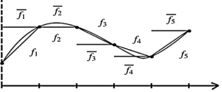
We start by introducing Rothe’s functions. They are piece-wise constant and piece-wise linear in time functions
and are constructed in the following way for i = 1, . . . , n (where n denotes the number of time steps)
φn(t ) =φci for t ∈ (ti −1, ti],
An(t ) = Ai An(t ) = Ai −1+(t − ti −1)δAi for t ∈ (ti −1, ti] An(0) = An(0) = A0,
un(t ) = ui un(t ) = ui −1+(t − ti −1)δui for t ∈ (ti −1, ti] un(0) = un(0) = u0,
βn(t ) =β(ui) βn(t ) =β(ui −1) + (t − ti −1)δβ(ui) for t ∈ (ti −1, ti] βn(0) =βn(0) =β(u0),
jn(t ) = ji λn(t ) =λi σπn(t ) =σπ(ui) for t ∈ (ti −1, ti].
For better interpretation we include a simple example of Rothe’s functions for a general function f (t ) inFig. 3.
Now, using these new notations we rewrite (25)–(27) in a continuous sense for the whole time interval [0, T ],
i.e. ( σπn(t −τ)∇φn, ∇ξ)T +( jn, ξ)Γ =0 for anyξ ∈ H 1(T )/R, (29) (σ πn(t −τ)∂tAn, ϕ)π + (µM(∇ × A n), ∇ × ϕ)Ω+ (σ πn(t −τ)∇φn, ϕ)T =0 for anyϕ ∈ XN,0, (30) (∂tβn, ψ)π+ (λ n∇un, ψ)π − ( Rr(σπn(t −τ)⏐⏐∂tAn+χT∇φn ⏐ ⏐ 2 ) , ψ) π =0 for anyψ ∈ H 1(π). (31)
Proposition 1. Suppose(21). Moreover assume that σ is globally Lipschitz continuous. Then there exist a scalar
Fig. 3. Rothe’s functions of a general function f (t).
by the same symbol again) such that
(i) un→u in C([0, T ]; L2(π)) ,
un(t )⇀ u(t) in H1(π), ∀t ∈ [0, T ],
un→u in L2((0, T ); L2(π)),
(ii) σπn →σπ(u), σπn(t −τ) → σπ(u) in L2((0, T ); L2(π)),
(iii) βn−βn →0 in C([0, T ]; (H1(π))∗
) ,
(iv) βn→β(u) in L2((0, T ); L2(π)),
(v) jn→ j in L2((0, T ); H−1/2(Γ ))
holds true for n → +∞.
Proof. (i) UsingLemma 5, we have∂tun ∈ L2((0, T ); L2(π)) and un ∈ C([0, T ]; H1(π)). Now, since H1(π) is
compactly embedded in L2(π), we apply well-known [23, Lemma 1.3.13] to conclude the first two statements of (i).
To prove the last one we only need to show that unand unhave the same limit in L2((0, T ); L2(π)). We may write
∫ T 0 ∥un−un∥2L2(π)dt = n ∑ i =1 ∫ ti ti −1 ∥ui−ui −1−(t − ti −1)δui∥2L2(π)dt = n ∑ i =1 ∫ ti ti −1 ∥δui(τ − t + ti −1)∥2L2(π)dt ⩽ τ2 n ∑ i =1 ∥δui∥2 L2(π)τ ⩽ Crτ2 n→∞−→0.
(ii) Sinceσ is supposed to be globally Lipschitz continuous and unconverges strongly to u in L2((0, T ); L2(π)),
we conclude thatσπn →σ(u) in the same space as well. The only thing left to be done is to show that σπ
n(t −τ) and
σπn(t ) share the same limit in L
2((0, T ); L2(π)). It holds ∫ T 0 σπn(t ) −σπn(t −τ) 2 L2(π)dt = n ∑ i =1 ∥σ(ui) −σ(ui −1)∥2L2(π)τ Li pschi t z ⩽ Cσ n ∑ i =1 ∥ui−ui −1∥2L2(π)τ =Cστ2 n ∑ i =1 ∥δui∥2 L2(π)τ ⩽ CσCrτ2 n→∞−→0.
(iii) Results fromLemma 5let us write
⏐ ⏐ (β n−βn, ψ)⏐⏐⩽ τ ∥∂tβn∥(H1(π))∗∥ψ∥H1(π)⩽ τ Cr∥ψ∥H1(π) and thereforeβn−βn (H1(π))∗⩽ τ Cr n→∞ −→0.
(iv) Taking into account the continuity ofβ and the fact that un converges strongly towards u, allow us to use
Lebesgue’s dominated convergence theorem to conclude thatβn →β(u) in L2((0, T ); L2(π)).
(v) Assuming that j is Lipschitz continuous in time, we write
∫ T 0 jn−j 2 H−1/2(Γ )dt = n ∑ i =1 ∫ ti ti −1 ∥ j (ti) − j (t )∥2H−1/2(Γ )dt⩽ Cτ 2 n→∞→ 0. □
Proposition 2. Suppose that all assumptions of Proposition 1 are satisfied. Then there exist a vector potential
A ∈ L2((0, T ); X
N,0) with∂tA ∈ L2((0, T ); L2(π)) and a sub-sequence of An(denoted by the same symbol again)
such that (i) An ⇀ A, ∇ × An ⇀ ∇ × A in L2((0, T ); L2(Ω)), µM(∇ × An)⇀ µM(∇ × A) in L2((0, T ); L2(Ω \ π)), An →A in C([0, T ]; L2(π)) , An(t )⇀ A(t), An(t )⇀ A(t) in H1(π), ∀t, ∂tAn⇀ ∂tA in L2((0, T ); L2(π)), (ii) M(∇ × An)⇀ M(∇ × A) in L2((0, T ); L2(π)), (iii) ∇ ×An → ∇ ×A in L2((0, T ); L2(π)), M(∇ × An) → M(∇ × A) in L2((0, T ); L2(π))
holds true for n → +∞.
Proof. (i)Lemma 4yields
∫ T 0 An 2 XN,0 dt⩽ C. The reflexivity of L2((0, T ); X
N,0) gives for a sub-sequence that An⇀ A in that space. One can easily see that
An ⇀ A, ∇ ×An ⇀ ∇ × A in L2((0, T ); L2(Ω)),
due to the density of C0∞(Ω ) in L2(Ω ), see [30, Thm. 2.6.1]. Take nowϕ ∈ C∞0 (Ω \π). Using µ ∈ H1(Ω \π) we
have ∫ T 0 ( µM(∇ × An), ϕ)Ωdt = ∫ T 0 ( µ∇ × An, ϕ)Ωdt = ∫ T 0 (An, ∇ × (µϕ))Ω dt.
Passing to the limit for n → ∞ we get lim n→∞ ∫ T 0 ( µ∇ × An, ϕ)Ωdt = ∫ T 0 (A, ∇ × (µϕ))Ωdt = ∫ T 0 (µ∇ × A, ϕ)Ω dt.
Using the density argument of C∞
0 (Ω \π) in L
2(Ω \π) we have
µM(∇ × An) =µ∇ × An⇀ µ∇ × A = µM(∇ × A) in L2((0, T ); L2(Ω \ π)).
Lemma 4together with XN,0⊂H1(Ω ) (cf. [19, Theorem 3.7]) imply
∫ T 0 ∥∂tAn∥2L2(π)dt⩽ C, An H1(π)⩽ An H1(Ω )⩽ C.
Employing [23, Lemma 1.3.13] we get for a sub-sequence that
An →A in C([0, T ]; L2(π))
An(t )⇀ A(t), An(t )⇀ A(t) in H1(π), ∀t
∂tAn ⇀ ∂tA in L2((0, T ); L2(π)).
(ii) The sequence M(∇ × An) is bounded in L2((0, T ); L2(Ω)). Therefore, there exists p from L2((0, T ); L2(Ω))
technique, cf. [31,18]. The general idea is based on monotone character of the vectorial field M. Let us investigate the following inequality 0⩽ ∫ T 0 (M(∇ × An) − M(b), ψµ (∇ × An−b )) Ωdt = I1+I2+I3+I4, (32) where I1= ∫ T 0 (M(∇ × An), ψµ∇ × An ) Ωdt, I2 = ∫ T 0 (M(b), ψµ∇ × An ) Ωdt, I3= ∫ T 0 (M(∇ × An), ψµb)Ωdt, I4 = ∫ T 0 (M(b), ψµb)Ωdt.
This inequality holds true for any b ∈ L2((0, T ); L2(Ω)) and any non-negative ψ ∈ C∞
0 (π). We want to pass to the
limit for n → ∞ in(32). We do it for each term in(32)separately.
It holds I1= ∫ T 0 (M(∇ × An), ψµ∇ × An ) Ωdt = ∫ T 0 (M(∇ × An), ψµ∇ × (An−A )) Ωdt + ∫ T 0 (M(∇ × An), ψµ∇ × A)Ωdt = ∫ T 0 (∇ × [ψµM(∇ × An)], An−A ) Ω dt + ∫ T 0 (M(∇ × An), ψµ∇ × A)Ωdt = ∫ T 0 ( ψ∇ × [µM(∇ × An) ] , An−A ) Ω dt + ∫ T 0 (∇ψ × [µM(∇ × An)], An−A ) Ωdt + ∫ T 0 (M(∇ × An), ψµ∇ × A)Ωdt.
We know that An →A in C([0, T ]; L2(π)) and ∂tAnis bounded in L2((0, T ); L2(π)). Therefore also An → A in
C([0, T ]; L2(π)). Thus, using µ ∈ H1(π), it is not difficult to see that
lim n→∞I1 = ∫ T 0 (p, ψµ∇ × A)Ωdt. Clearly lim n→∞I2 = ∫ T 0 (M(b), ψµ∇ × A)Ωdt lim n→∞I3 = ∫ T 0 (p, ψµb)Ωdt lim n→∞I4 = ∫ T 0 (M(b), ψµb)Ωdt.
Assembling these auxiliary results we arrive at
lim n→∞ ∫ T 0 (M(∇ × An) − M(b), ψµ (∇ × An−b )) Ω dt = ∫ T 0 (p − M(b), ψµ (∇ × A − b))Ωdt⩾ 0.
Since b was taken as an arbitrary element of L2((0, T ); L2(Ω)) we choose it as b = ωq + ∇ × A, where
q ∈ L2((0, T ); L2(Ω)) and ω > 0. Using this substitution in the equation above we obtain
∫ T 0 (p − M(∇ × A + ωq), µψ (−ωq))Ωdt ⩾ 0 / · 1 ω, ∫ T 0 (p − M(∇ × A + ωq), µψ (−q))Ωdt ⩾ 0 / ω → 0, ∫ T 0
(p − M(∇ × A), µψ (−q))Ωdt ⩾ 0 / q is arbitrary, hence we choose q = −q,
∫ T
0
(p − M(∇ × A), µψ (−q))Ωdt ⩽ 0.
The conclusion is that ∫0T (p − M(∇ × A), µψq)Ω dt = 0 for any non-negative ψ ∈ C
∞
0 (π) and every q ∈
L2((0, T ); L2(Ω)). Hence p = M(∇ × A) a.e. in (0, T ) × π and M(∇ × An)⇀ M(∇ × A) in L2((0, T ); L2(π)).
(iii) Analogously as in (ii) using the strong monotonicity of M (k1) we conclude 0 = lim n→∞ ∫ T 0 (M(∇ × An) − M(∇ × A), µψ (∇ × An− ∇ ×A )) Ωdt ⩾ limn→∞cM ∫ T 0 (µψ, ⏐⏐∇ ×An− ∇ ×A ⏐ ⏐ 2) Ωdt ⩾ 0. Therefore limn→∞ ∫T 0 (µψ, ⏐⏐∇ ×An− ∇ ×A ⏐ ⏐ 2) Ω dt = 0 for every 0 ⩽ ψ ∈ C∞ 0 (π), which implies ∇ × An →
∇ ×A in L2((0, T ); L2(π)). Vectorial field M is also Lipschitz continuous, hence M(∇ × A
n) → M(∇ × A) in
L2((0, T ); L2(π)) as well. □
Now, we are in a position to state our main result.
Theorem 1. Suppose that all assumptions of Proposition1are satisfied. Then there exist a solution-triplet {φ, A, u}
whereφ ∈ L2((0, T ); H1(T )/R), A ∈ L2((0, T ); XN,0) with∂tA ∈ L2((0, T ); L2(π)) and u ∈ C([0, T ]; L2(π)) ∩
L∞((0, T ); H1
0(π)) with ∂tu ∈ L2((0, T ); L2(π)) and a sub-sequences of φn, An and un (denoted by the same
symbol again) such that
(i) φ and u solve (19)
(ii) ∇φn→ ∇φ in L2((0, T ); L2(T ))
(iii) φ, u and A solve (18)
(iv) ∂tAn →∂tA in L2((0, T ); L2(π))
(v) φ, u and A solve (20)
holds true for n → +∞.
Proof. (i) Existence of a potentialφ ∈ H1(T )/R such that ∇φ
n ⇀ ∇φ in L2((0, T ); L2(T )) follows from the
reflexivity of L2((0, T ); L2(T )). The function φ has in fact a zero mean over T , cf. proof ofLemma 1.
Takeξ ∈ H1(T )/R in(29)and integrate in time
∫ ζ 0 (σ πn(t −τ)∇φn, ξ)T dt + ∫ ζ 0 ( jn, ξ)Γ dt = 0.
Thanks toProposition 1(ii) and (v), we pass to the limit for n → ∞ to get
∫ ζ 0 (σπ(u)∇φ, ξ)T dt + ∫ ζ 0 ( j, ξ)Γ dt = 0.
(ii) It holds 0⩽ σ∗ ∫ T 0 ∇ [ φn−φ] 2 L2(T )dt ⩽ ∫ T 0 (σ πn(t −τ)∇ [φn−φ] , ∇ [φn−φ])T dt = ∫ T 0 ( σπn(t −τ)∇φ, ∇φ)T dt + ∫ T 0 ( σπn(t −τ)∇φn, ∇φn ) T dt −2 ∫ T 0 (σ πn(t −τ)∇φn, ∇φ)T dt (29) = ∫ T 0 ( σπn(t −τ)∇φ, ∇φ)T dt − ∫ T 0 ( jn, φn ) Γ dt −2 ∫ T 0 (σ πn(t −τ)∇φn, ∇φ)T dt.
Passing to the limit, we conclude
0⩽ lim n→∞σ∗ ∫ T 0 ∇ [φ n−φ] 2 L2(T )dt ⩽ − ∫ T 0 (σπ(u)∇φ, ∇φ)T dt − ∫ T 0 ( j, φ)Γ dt (i ) =0. Therefore, ∇φn → ∇φ in L2((0, T ); L2(T )).
(iii) We integrate(30)in time
∫ ζ 0 ( σπn(t −τ)∂tAn, ϕ)π dt + ∫ ζ 0 ( µM(∇ × An), ∇ × ϕ)Ωdt + ∫ ζ 0 ( σπn(t −τ)∇φn, ϕ)T dt = 0.
UsingProposition 1(ii),Proposition 2andTheorem 1(ii), we pass to the limit for n → ∞ to see
∫ ζ 0 (σπ(u)∂tA, ϕ)π dt + ∫ ζ 0 (µM(∇ × A), ∇ × ϕ)Ωdt + ∫ ζ 0 (σπ(u)∇φ, ϕ)T dt = 0.
Thus,φ, u and A solve(18).
(iv) The strong convergence of ∇ × An → ∇ ×A in L2((0, T ); L2(π)) is guaranteed byProposition 2(iii). Let us
take anyζ ∈ [0, T ] such that ∇ × An(ζ) → ∇ × A(ζ) in L2(π). This set is dense in [0, T ]. Take any non-negative
ψ ∈ C∞
0 (π). We use the positiveness of σ to estimate the following
0⩽ σ∗ ∫ ζ 0 ∫ πψ|∂t An−∂tA|2dx dt⩽ ∫ ζ 0 ∫ πψσπn (t −τ)|∂tAn−∂tA|2dx dt = −2 ∫ ζ 0 (ψσ πn(t −τ)∂tAn, ∂tA ) πdt + ∫ ζ 0 (ψσ πn(t −τ)∂tA, ∂tA ) π dt + ∫ ζ 0 (ψσ πn(t −τ)∂tAn, ∂tAn ) π dt.
We use Lebesgue’s dominated convergence theorem combined withProposition 1(ii) andProposition 2(i) to pass to
the limit for n → ∞ in the first two terms lim n→∞ −2 ∫ ζ 0 ( ψσπn(t −τ)∂tAn, ∂tA ) π dt = −2 ∫ ζ 0 (ψσπ(u)∂tA, ∂tA)π dt, lim n→∞ ∫ ζ 0 (ψσ πn(t −τ)∂tA, ∂tA ) π dt = ∫ ζ 0 (ψσπ(u)∂tA, ∂tA)π dt.
We assume thatζ ∈ (tj −1, tj] and use variational formulation(30)to rewrite the third term as ∫ ζ 0 (ψσ πn(t −τ)∂tAn, ∂tAn ) πdt = − ∫ ζ 0 (µM(∇ × A n), ∇ × (ψ∂tAn))Ωdt − ∫ ζ 0 (σ πn(t −τ)∇φn, ψ∂tAn ) T dt = − ∫ ζ 0 ( ψµM(∇ × An), ∇ × ∂tAn ) Ωdt − ∫ ζ 0 ( µM(∇ × An), ∇ψ × ∂tAn ) Ω dt − ∫ ζ 0 ( σπn(t −τ)∇φn, ψ∂tAn ) T dt =:R1+R2+R3.
Let us rewrite the first term on the RHS and examine it closely
R1= − ∫ tj 0 ( ψµM(∇ × An), ∇ × ∂tAn ) Ωdt + ∫ tj ζ ( ψµM(∇ × An), ∇ × ∂tAn ) Ωdt = − tj ∑ i =1 ∫ Ω ψµM(∇ × Ai) ·(∇ × Ai− ∇ ×Ai −1)) dx + ∫ tj ζ (∇ × (ψµM(∇ × An)), ∂tAn ) Ωdt (22) ⩽ − tj ∑ i =1 ∫ Ω ψµ {ΦM(∇ × Ai) − ΦM(∇ × Ai −1)} dx + ∫ tj ζ (∇ψ × (µM(∇ × An)), ∂tAn ) Ωdt + ∫ tj ζ ( ψ∇ × (µM(∇ × An) ) , ∂tAn ) Ωdt = − ∫ Ω ψµΦM(∇ × Aj) dx + ∫ Ω ψµΦM(∇ × A0) dx + ∫ tj ζ (∇ψ × (µM(∇ × An)), ∂ tAn ) Ωdt + ∫ tj ζ (ψ∇ × (µM(∇ × A n) ), ∂ tAn ) Ωdt = − ∫ Ω ψµΦM(M(∇ × An(ζ)) dx + ∫ Ω ψµΦM(∇ × A0) dx + ∫ tj ζ (∇ψ × (µM(∇ × An)), ∂ tAn ) Ωdt + ∫ tj ζ (ψ∇ × (µM(∇ × A n) ), ∂ tAn ) Ωdt.
Now, we are able to pass to the limit for n → ∞ to find lim n→∞R2 = − ∫ ζ 0 (µM(∇ × A), ∇ψ × ∂tA)Ω dt, lim n→∞R3 = − ∫ ζ 0 (σπ(u)∇φ, ψ∂tA)T dt, and lim n→∞R1⩽ − ∫ Ω ψµΦM(∇ × A(ζ)) dx + ∫ Ω ψµΦM(∇ × A(0)) dx = − ∫ ζ 0 ∫ Ω ψµdΦM(∇ × A) dt dx dt = − ∫ ζ 0 ∫ Ω ψµM(∇ × A) · ∂t(∇ × A) dx dt = − ∫ ζ 0 (µM(∇ × A), ψ∇ × (∂tA))Ω dt.
Thus lim n→∞R1 +R2+R3⩽ − ∫ ζ 0 (µM(∇ × A), ∇ × (ψ∂tA))Ωdt − ∫ ζ 0 (σπ(u)∇φ, ψ∂tA)T dt (18) = ∫ ζ 0 (ψσπ(u)∂tA, ∂tA)π dt.
Thus, collecting all estimates above, we see that
0⩽ lim n→∞ ∫ ζ 0 ∫ πψ|∂t An−∂tA|2dx dt ⩽ 0.
Please note that this is valid for any non-negativeψ ∈ C∞0 (π). Since the set of ζ ∈ [0, T ] for which ∇ × An(ζ) →
∇ ×A(ζ) in L2(Ω) is dense in [0, T ], we achieve a strong convergence of ∂
tAnin L2((0, T ); L2(π)) i.e. ∂tAn →∂tA
in L2((0, T ); L2(π)).
(v) Takeψ ∈ H1(π) in(31)and integrate in time
(β n(t ) −βn(0), ψ)π+ (β n(t ) −βn(t ), ψ)π + ∫ t 0 (λ n∇un, ∇ψ)π ds = ∫ t 0 ( Rr(σπn(s −τ)⏐⏐∂tAn+χT∇φn ⏐ ⏐ 2 ) , ψ) πds.
Using Lebesgue’s dominated convergence theorem, together withProposition 1(ii),Theorem 1(ii) and (iv) enables
passing to the limit for n → ∞ in the RHS of the equation above lim n→∞ ∫ t 0 ( Rr(σπn(s −τ)⏐⏐∂tAn+χT∇φn ⏐ ⏐ 2 ) , ψ) πds = ∫ t 0 ( Rr(σπ(u) ⏐ ⏐∂tA +χT∇φ⏐⏐ 2 ) , ψ) π ds.
Proposition 1let us pass to the limit for n → ∞ on the LHS. Note that term(βn(t ) −βn(t ), ψ)π vanishes since
limn→∞
(
βn(t ) −βn(t ), ψ)π =0 for every t ∈ [0, T ]. Therefore gathering all results above brings us to
(β(u(t)) − β(u(0)), ψ)π+ ∫ t 0 (λ∇u, ∇ψ)πds = ∫ t 0 ( Rr(σπ(u) ⏐ ⏐∂tA +χT∇φ⏐⏐ 2 ) , ψ) π ds.
The only thing left to be done to finish the proof is differentiating with respect to time. Thus, we see thatφ, u and A
indeed solve(20). □
4. Numerical simulation
To support our proposed numerical scheme(28)obtained from the variational formulation (27), (26), (25)we
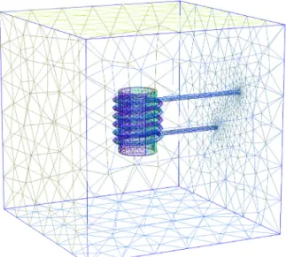
provide a numerical simulation of induction hardening process. The domain used in the simulation is reported in
Fig. 4. This domain is more complex than its simplified version inFig. 1, but our theoretical results for this type hold
regardless, because the inclusion XN,0 ⊂ H1(Ω ) holds true also for convex domains (without a smooth boundary),
cf. [21, Theorem 2.17]. Since we want our simulation to be realistic we use physical constants. Unknown functions
representing nonlinearities are chosen accordingly to satisfy(21)
σπ(u) = 2σc+σc ( 2 − ( 1 + 1 1 + u )1+u) , β(u) = βc √ u, M(∇ × A) =(1 + e−|∇×A|) ∇ × A, σc, βc, µ, λ H⇒ Physical constants, T = 0.02, A0=0, u0=293 Kelvin.
We split the time interval [0, T ] in 1280 equidistant parts (τ = 1.5625e10−5) and use the open source finite element
Fig. 4. Meshed domain.
(a) Magnetic induction field. (b) Temperature.
Fig. 5. Reference solutions in time t = 0.015.
and(27)at each time step, after spatial discretization using Whitney finite elements on tetrahedra (edge elements
for the magnetic vector potential, nodal elements for the electric scalar potential and the temperature) [34]. The
Neumann boundary condition in(14)and(17)is simply treated by adding the corresponding surface term arising
from integration by parts in the weak formulation. The mesh contained 26 765 tetrahedra, leading to a total of 29 714 unknowns. We denote obtained solutions for the magnetic induction field and the temperature function as reference solutions br e f and ur e f, respectively. Typical solutions are plotted inFig. 5.
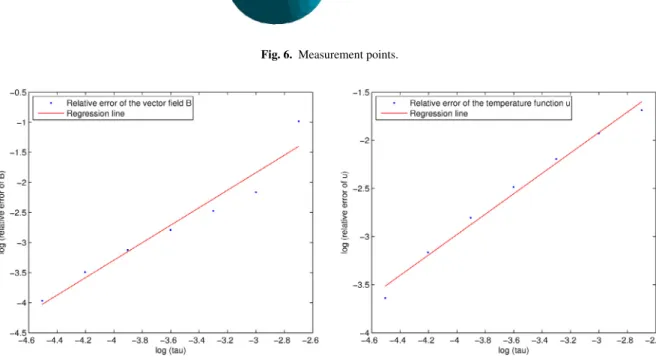
To show that our scheme is converging to br e f and ur e f we compute other numerical solutions for number of time
steps 10, 20, 40, 80, 160, 320 and 640 and compare them with br e f and ur e f. We analyze these solutions in certain
measurement points of our domain (seeFig. 6) and at certain time steps, namely ti =0.002i, where i = 1, . . . , 10.
Fig. 6. Measurement points.
(a) Relative error of the magnetic induction field B with respect to a decreasing time stepτ.
(b) Relative error of the temperature function u with respect to a decreasing time stepτ.
Fig. 7. Logarithmically scaled plot of a decreasing time stepτ and the relative errors.
in the following manner ⏐ ⏐br e f ⏐ ⏐ = ∑ Pj∈P 10 ∑ i =1 ⏐ ⏐br e f(Pj, ti) ⏐ ⏐ ⏐ ⏐ur e f ⏐ ⏐ = ∑ Pj∈P 10 ∑ i =1 ⏐ ⏐ur e f(Pj, ti) ⏐ ⏐ ⏐ ⏐br e f −bn ⏐ ⏐ = ∑ Pj∈P 10 ∑ i =1 ⏐ ⏐br e f(Pj, ti) − bn(Pj, ti) ⏐ ⏐ ⏐ ⏐ur e f −un ⏐ ⏐ = ∑ Pj∈P 10 ∑ i =1 ⏐ ⏐ur e f(Pj, ti) − un(Pj, ti) ⏐ ⏐ rel bn = ⏐ ⏐br e f −bn ⏐ ⏐ ⏐ ⏐br e f ⏐ ⏐ rel un= ⏐ ⏐ur e f −un ⏐ ⏐ ⏐ ⏐ur e f ⏐ ⏐ ,
where P is the set of measurement points. Please bear in mind that the index n refers to the numerical solution
computed on a mesh with 2n−1·10 time steps. The evolution of these errors with increasing number of time steps can
be seen inFig. 7.
If the error of a given numerical solution fτ from the exact solution f depends smoothly on a time stepτ then
there exist an error coefficient D such that fτ− f = Dτp+O(τp+1),
where p represents the order of convergence. Using the fact that the difference of fτ − fτ/2decays to zero with the
same speed as fτ− f we can estimate the order of convergence without knowing the exact solution f , i.e.
fτ− fτ/2 fτ/2− fτ/4 = Dτp−D(τ/2)p+O(τp+1) D(τ/2)p−D(τ/4)p+O(τp+1) =2 p+O(τ), which gives us log2 ( f τ− fτ/2 fτ/2− fτ/4 ) =p +O(τ).
Applying the formula above to our numerical solutions we obtain an estimation for the order of convergence of bn
and un
pu≈0.9830 and pb≈1.0010.
This provides a strong indication that the convergence of our numerical scheme is linear. 5. Conclusion
We have provided a derivation of a mathematical model of induction hardening process with inclusion of a nonlinear relation between the magnetic field and the magnetic induction field. We have also proven an existence of a weak solution of our model.
To support the theoretical results we have coded the numerical scheme implied by a variational formulation and ran few simulations. However, we did not have an analytic solution. Numerical solutions are therefore compared with a numerical reference one computed on a fine reference mesh. Afterwards we have investigated how the numerical solutions computed for the increasing number of time steps (starting at 10) were behaving according to the reference
solutions br e f and ur e f. We have obtained an improving match with increasing number of time steps. Since we do not
have a proof of a unique solution of our model we could not prove the convergence of the scheme rigorously. However the numerical experiments suggest that the scheme might really be convergent.
In the following work we would like to provide a proof of a unique solution. The coupling between the vector
potential equation and the heat equation in the form of the temperature dependent functionσ(u) prevents us from
obtaining the desired energy estimates needed to prove the uniqueness of the solution and therefore it still remains an open problem.
Acknowledgments
J. Chovan was supported by the BOF-project no. 01J04113, Ghent University, Belgium. Ch. Geuzaine and M. Slodiˇcka were partially supported by the IAP P7/02-project of the Belgian Science Policy.
References
[1] C.M. Elliott, S. Larsson, A finite element model for the time-dependent Joule heating problem, Math. Comp. 64 (212) (1995) 1433–1453.
[2] G. Akrivis, S. Larsson, Linearly implicit finite element methods for the time-dependent Joule heating problem, BIT 45 (2005) 429–442.
[3] J. Barglik, I. Doležel, P. Karban, B. Ulrych, Modelling of continual induction hardening in quasi-coupled formulation, Compel 24 (1) (2005) 251–260.
[4] A. Bermúdez, D. Gómez, M. Muñiz, P. Salgado, Transient numerical simulation of a thermoelectrical problem in cylindrical induction heating furnaces, Adv. Comput. Math. 26 (1–3) (2007) 39–62.
[5] D. Sun, V. Manoranjan, H.-M. Yin, Numerical solutions for a coupled parabolic equations arising induction heating processes, Discrete Contin. Dyn. Syst. 2007 (2007) 956–964.
[6] H. Gao, Optimal error analysis of Galerkin fems for nonlinear Joule heating equations, J. Sci. Comput. 58 (3) (2014) 627–647.
[7] H.-M. Yin, Global solutions of Maxwell’s equations in an electromagnetic field with a temperature-dependent electrical conductivity, European J. Appl. Math. 5 (1994) 57–64.
[8] H.-M. Yin, On Maxwell’s equations in an electromagnetic field with the temperature effect, SIAM J. Math. Anal. 29 (3) (1998) 637–651.
[9] H.-M. Yin, Regularity of weak solution to Maxwell’s equations and applications to microwave heating, J. Differential Equations 200 (1) (2004) 137–161.
[10] D. Sun, V. Manoranjan, H.-M. Yin, Numerical solutions for a coupled parabolic equations arising induction heating processes, Dyn. Syst. (2007) 956–964.
[11] M. Bie´n, Global solutions of the non-linear problem describing Joule’s heating in three space dimensions, Math. Methods Appl. Sci. 28 (9) (2005) 1007–1030.
[12] D. Hömberg, A mathematical model for induction hardening including mechanical effects, Nonlinear Anal. RWA 5 (1) (2004) 55–90.
[13] D. Hömberg, T. Petzold, E. Rocca, Analysis and simulations of multifrequency induction hardening, Nonlinear Anal. RWA 22 (0) (2015) 84–97.
[14] A. Bossavit, J.F. Rodrigues, On the electromagnetic “induction heating” problem in bounded domains, Adv. Math. Sci. Appl. 4 (1) (1994) 79–92.
[15] J. Chovan, M. Slodiˇcka, Induction hardening of steel with restrained joule heating and nonlinear law for magnetic induction field: Solvability, JCAM 311 (2017) 630–644.
[16] M. Slodiˇcka, J. Chovan, Solvability for induction hardening including nonlinear magnetic field and controlled joule heating, Appl. Anal. Available online athttp://dx.doi.org/101080/0003681120161243661.
[17] L.D. Landau, E.M. Lifshitz, Electrodynamics of Continuous Media, Vol. 8, Oxford: Pergamon Press, 1960.
[18] M. Vajnberg, Variational Method and Method of Monotone Operators in the Theory of Nonlinear Equations, John Wiley & Sons, 1973.
[19] V. Girault, P.-A. Raviart, Finite Element Methods for Navier–Stokes Equations, Springer, Berlin, 1986.
[20] P. Monk, Finite Element Methods for Maxwell’s Equations, Oxford University Press Inc., New York, 2003.
[21] C. Amrouche, C. Bernardi, M. Dauge, V. Girault, Vector potentials in three-dimensional non-smooth domains, Math. Methods Appl. Sci. 21 (9) (1998) 823–864.
[22] R.A. Adams, Sobolev Spaces, Academic Press, Springer Verlag, 1978.
[23] J. Kaˇcur, Method of Rothe in Evolution Equations, in: Teubner Texte zur Mathematik, vol. 80, Teubner, Leipzig, 1985.
[24] K. Rektorys, The Method of Discretization in Time and Partial Differential Equations, in: Mathematics and Its Applications (East European Series), vol. 4, D. Reidel Publishing Company, Dordrecht - Boston - London, 1982.
[25] J. Neˇcas, Introduction to the Theory of Nonlinear Elliptic Equations, John Wiley & Sons Ltd, Chichester, 1986.
[26] M. Slodiˇcka, S. Dehilis, A nonlinear parabolic equation with a nonlocal boundary term, J. Comput. Appl. Math. 233 (12) (2010) 3130–3138.
[27] T. Roubíˇcek, Nonlinear Partial Differential Equations with Applications, Birkhäuser, Berlin, 2005.
[28] G.J. Minty, On a “monotonicity” method for the solution of nonlinear equations in Banach spaces, Proc. Natl. Acad. Sci. 50 (6) (1963) 1038–1041.
[29] F.E. Browder, Nonlinear elliptic boundary value problems. ii, Trans. Amer. Math. Soc. 117 (1965) 530–550.
[30] A. Kufner, O. John, S. Fuˇcík, Function Spaces, Monographs and Textbooks on Mechanics of Solids and Fluids, Noordhoff International Publishing, Leyden, 1977.
[31] L.C. Evans, Partial Differential Equations, Vol. 19, American Mathematical Society, RI, 1998.
[32] C. Geuzaine, J.-F. Remacle, Gmsh: a three-dimensional finite element mesh generator with built-in pre- and post-processing facilities, Internat. J. Numer. Methods Engrg. 79 (11) (2009) 1309–1331.
[33] P. Dular, C. Geuzaine, F. Henrotte, W. Legros, A general environment for the treatment of discrete problems and its application to the finite element method, IEEE Trans. Magn. 34 (5) (1998) 3395–3398.
[34] A. Bossavit, Computational electromagnetism, in: Variational Formulations, Complementarity, Edge Elements, in: Electromagnetism, vol. 18, Academic Press, Orlando, FL, 1998.