A dynamics based method for accelerometer-only navigation of a spinning projectile

A Dynamics Based Method for Accelerometer-Only

Navigation of a Spinning Projectile

by

Paul James Goulart

Submitted to the Department of Aeronautics and Astronautics in partial fulfillment of the requirements for the degree of

Master of Science in Aeronautics and Astronautics at the

MASSACHUSETTS INSTITUTE OF TECHNOLOGY

September 2001

@

The author hereby grants to MIT permission to reproduce and to distribute publicly paper and electronic copies of this thesis document in whole or in part.

Author ...

Department of Aeronautics and Astronautics September 1, 2001 C ertified by ... Certified by... Accepted by...

. . .

...

...

...

...

.

...

. . . .

Prof. Steven H. Hall Professor of Aeronautics and Astronautics Thesis Supervisor j A A.A MASSACHUSETTS INSTITUTE MASSACHUSETTS NSTITUTE OF TECHNOtOGY

AUG

1 3 2002

Prof. Wallace E. Vander Velde Professor of Aeronautics and Astronautics IChair, Committee on Graduate Students

A Dynamics Based Method for Accelerometer-Only

Navigation of a Spinning Projectile

by

Paul James Goulart

Submitted to the Department of Aeronautics and Astronautics on September 1, 2001, in partial fulfillment of the

requirements for the degree of

Master of Science in Aeronautics and Astronautics

Abstract

A method of navigating a gun-launched, spinning projectile using only

accelerome-ters is presented. A linear combination of the outputs of a general configuration of at least 12 accelerometers is shown to provide measurements of angular acceleration

and angular rate products of the form w and oxy These measurements are used

in the development of a 12 state, extended Kalman filter to estimate position, ve-locity, attitude, and angular rate, with twelve additional states included to estimate accelerometer biases.

Assumptions about the dynamic behavior of the vehicle are used to assist in attitude estimation. These assumptions come in two parts. First, that the nose of the vehicle remains pointed along the air-relative velocity vector during flight. Second, that the vehicle lateral angular rates have a secular component due to the vehicle pitching over during flight to maintain this alignment. A digital filter is used to isolate the secular pitch-over component of the estimated rate in an intermediate, non-rolling frame. These dynamics-based estimates are then incorporated as measurements in the navigation filter.

A configuration of 12 accelerometers arranged on the faces of a 10 cm cube is used

in a six degree of freedom simulation to navigate a projectile spinning at 2 Hz. The navigation filter is shown to reliably estimate angular rates with biases as large as 1 g. Bias state estimation is also shown to compensate for instrument misalignments up to 1 degree. Using the dynamics-based measurements, the navigation filter successfully estimates projectile roll attitude to within 20 degrees for instrument random walk errors up to 2.5 milli-g/v/Hz.

Thesis Supervisor: Dr. Matthew Bottkol

Title: Technical Staff, Charles Stark Draper Laboratory Thesis Supervisor: Prof. Steven R. Hall

Acknowledgments

I would like to thank all of the people who have helped and supported me during the writing of this thesis, and during my time at MIT.

Thanks to the many Draper staff who I have had the opportunity of working with over the last two years: Chris D'Souza, Chris Stoll, Time Brand, Don Gustafson, George Schmidt, Tom Thorvaldsen, and Dave Geller. Special thanks to Dave for letting me borrow the same book so many times.

Thanks very much to my thesis supervisor at Draper, Matt Bottkol, for his time, advice, and encouragement, and for helping me to find a good topic. Thanks also to my thesis advisor, Prof. Steven Hall, for his many helpful suggestions, comments, and clarifications.

Thanks to the many other Draper Fellows who I've spent the last two years with: Andre Girerd, John Stedl, Andrew Grubler, and Raja Chari. Thanks especially to Jeremy Rea for studying for the quals with me. Many thanks also to all of the friends I have made in Cambridge and at MIT over the last few years.

Thanks to my family for their continuing love, support, and encouragement. Finally, thanks to my fiancee Emma for her love, patience, and sacrifice.

ACKNOWLEDGMENT

This thesis was prepared at The Charles Stark Draper Laboratory, Inc., under

NAVSEA PMS529 Contract N00024-01-C-5247.

Publication of this thesis does not constitute approval by Draper or the sponsoring agency of the findings or conclusions contained herein. It is published for the exchange and stimulation of ideas.

Permission is hereby granted by the author to the Massachusetts Institute of Tech-nology to reproduce any ar all of this thesis.

Contents

1 Introduction 15

1.1 B ackground . . . . 15

1.2 Thesis Objectives and Overview . . . . 16

2 Simulation Environment 19 2.1 Equations of Motion . . . . ... . . . . 19 2.2 Atmospheric Model . . . . 21 2.3 Aerodynamic Forces . . . . 21 3 Measurement Transformations 25 3.1 Accelerometer Outputs . . . . 25

3.2 Deterministic Solution for Angular Rates . . . . 27

3.3 Instrument Configuration . . . . 28

4 Filter Implementation 31 4.1 Kalman Filter Equations . . . . 32

4.2 State Transition Equations . . . . 33

4.2.1 Position Perturbation State . . . . 34

4.2.2 Velocity Perturbation State . . . . 34

4.2.3 Attitude Perturbation State . . . . 34

4.2.4 Rate Perturbation State . . . . 35

4.2.5 Instrument Errors . . . . 36

4.2.6 Effect of Sensor Misalignments . . . . 37

4.3 Measurement Equations . . . . 38

4.3.1 Rate Measurements . . . . 38

4.3.2 GPS Measurement . . . . 40

4.4 State Update Equations . . . . 41

4.4.1 Propagating the Reference State . . . . 41

4.4.2 Applying the Error States . . . . 41

4.5 Managing Rate Linearization Error . . . . 42

5 Dynamics Based Navigation 45 5.1 Gravity Turn Rate . . . . 45

5.2 Velocity Alignment Pseudo-Measurement . . . . 46

5.3.1 Isolating the Pitch-Over Rate Component . . . . . 6 Results

6.1 Rate Estimation Performance . . . .

6.1.1 Unbiased Rate Estimation . . . .

6.1.2 Rate Estimation with Biases . . . .

6.1.3 Rate Estimation with Scale Factor and

6.2 IIR Filter Design . . . .

6.2.1 Lateral Rate Frequency Content . . . .

6.2.2 Filter Specifications . . . .

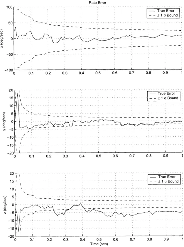
6.2.3 Filter Performance . . . .

6.3 Attitude Estimation Performance . . . .

7 Conclusions

7.1 Sum m ary . . . .

7.2 Suggestions for Further Research . . . .

A Dynamics Model

A. 1 General Vehicle Dynamics . . . . A.2 Linearized Aerodynamics Model . . . . A.3 Estimating Velocity Vector Misalignment . . .

. . . .

. . . .

. . . .

. . . .

. . . .

. . . .

. . . .

. . . .

List of Figures

2-1 View of Simulation Environment . . . . 20

2-2 Typical vehicle trajectory . . . . 22

3-1 Accelerometer configuration . . . . 29

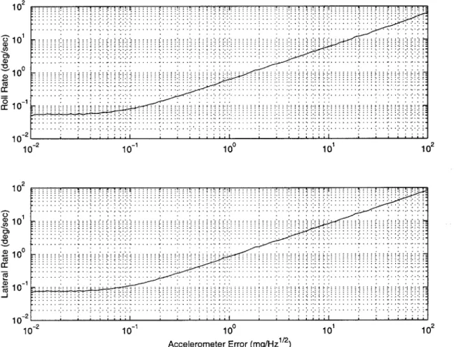
6-1 Rate estimation error vs accelerometer oUr . . . . 53

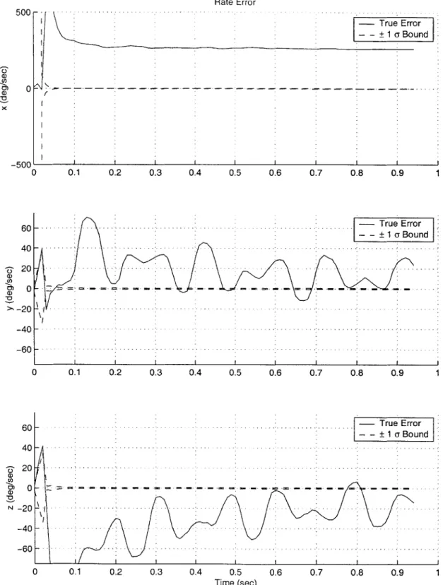
6-2 Example - Rate estimation divergence . . . . 54

6-3 Example -Rate divergence correction using EKF compensation technique 55 6-4 Roll rate estimation error vs bias - no EKF compensation . . . . 56

6-5 Roll rate estimation error vs bias - partial EKF compensation . . . . 56

6-6 Roll rate estimation error vs bias - full EKF compensation . . . . 57

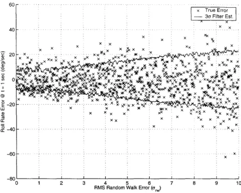
6-7 Roll rate estimation error vs Urw . . . . 58

6-8 Lateral rate estimation error vs o r _{. . . . 58}

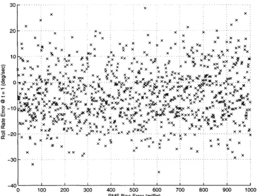
6-9 Roll rate estimation error vs bias . . . . 59

6-10 Lateral rate estimation error vs bias . . . . 59

6-11 Roll rate estimation error vs bias . . . . 60

6-12 Lateral rate estimation error vs bias . . . . 60

6-13 Roll rate estimation error vs scale factor error . . . . 62

6-14 Lateral rate estimation error vs scale factor error . . . . 62

6-15 Roll rate estimation error vs misalignment error - no process noise . . 63

6-16 Lateral rate estimation error vs misalignment error - no process noise 63 6-17 Roll rate estimation error vs misalignment error - no process noise . . 64

6-18 Lateral rate estimation error vs misalignment error - no process noise 64 6-19 Lateral rate PSD for true rates . . . . 65

6-20 Lateral rate PSD for different levels of Urw . . . . 66

6-21 IIR filter design . . . . 67

6-22 Gravity-turn vector (i) error convergence (Urw = 0.5 milli-g/ Hz) 68 6-23 Steady-state gravity-turn vector (i) error . . . . 68

6-24 Roll angle estimation error vs initial error. (arm = 0.5 milli-g/ Hz) . 70 6-25 Roll angle estimation error distribution. (o, = 0.5 milli-g/ Hz) . . 70

6-26 Roll angle estimation error vs initial error. ( = 1 milli-g/Hz) 1r . . 71

6-27 Roll angle estimation error distribution. (a, =

1

Hz)

6-28 Roll angle estimation error vs initial error. (a,, = 2.5 milli-g/ Hz) . 72 6-29 Roll angle estimation error distribution. (ar, = 2.5 milli-g/Hz) . . 72

6-30 Roll angle estimation error vs initial error. (arw = 5 milli-g/Hz) . . 73

List of Tables

Nominal launch conditions . . . .

Vehicle properties . . . . Atmospheric conditions . . . . Aerodynamic coefficients . . . . Accelerometer configuration . . . .

Rate estimation results summary . . . . Roll attitude estimation results summary . . . .

Accelerometer error requirements and initial estimate

2.1 2.2 2.3 2.4 3.1 6.1 6.2 7.1 . . . . 21 . . . . 21 . . . . 22 . . . . 23 . . . . 28 . . . . 52 . . . . 69 . . . . 76

Symbols

AIB 3 x 3 body to inertial frame transformation matrix

ai total acceleration of ith accelerometer

E pseudo-inverse of accelerometer transformation matrix. E = M#

F _{state transformation matrix (continuous time)}

fi

g gravity vector

C matrix of measurement partial derivatives

I identity matrix or 3 x 3 inertia tensor

I, _{roll component isolation matrix. I, = diag}

_([

It _{transverse component isolation matrix. It = diag}

_([

K Kalman gain matrix

M accelerometer transformation matrix. r/ = Mf

P covariance matrix

Q

q _{inertial to body frame attitude quaternion. q = [q, qs]}

R measurement noise matrix

ri projectile position (inertial frame)

ri body frame position of ith accelerometer

SB linear acceleration at origin of body reference frame

vB projectile velocity (body frame)

vi projectile velocity (inertial frame)

W matrix of angular rate products [o

x][w

wS vector of rate square terms, i.e. w2

X

w, _{vector of rate cross terms, i.e. wxwy}

z measurement for Kalman filter

aB angular acceleration in body frame

#

-y vehicle flight path angle

77 vector of vehicle accelerations and rate products 6. body frame orientation of ith accelerometer Ai misalignment vector for ith accelerometer

v white noise process

orw accelerometer random walk error

<b state transformation matrix (discrete time)

4p attitude perturbation state

WB angular rate in body frame

Notation x scalar quantity

X matrix quantity X vector quantity z estimated value of x

.: nominal or reference value of x tr(X) trace of matrix X

E[x] expected value of x

0 -xx xy [xx] matrix form of the cross product. [xx] = x 0 -x

Chapter 1

Introduction

1.1

Background

For several years, munitions research programs underway at Draper Laboratory such as the Extended Range Guided Munitions Demonstration (ERGM Demo) [4], and the Competent Munition Advanced Technology Demonstration (CMATD), have sought to develop low cost guidance and navigation systems for spin-stabilized, gun-launched projectiles. The environments in which these systems must operate present several unique challenges for inertial navigation.

During the boost phase, gun-launched systems can experience shocks in excess of 10,000 g, which can cause significant changes to instrument alignment, bias, scale factors, etc., requiring significant in-flight instrument calibration [5]. On the ERGM system, the guidance and control system requires that the navigation system be ca-pable of providing an initial estimate of local vertical (termed down determination) to within approximately 15-20 degrees, without the benefit of any kind of external measurement such as GPS. Systems such as ERGM solve this problem by noting that the lateral rates of the projectile must have a component attributable to the slow pitching over of the vehicle as it seeks to remain aligned with the flight path [6, 8].

Typically, inertial navigation systems rely on a combination of high quality inertial instrumentation and precise knowledge of initial conditions for attitude determina-tion. In these systems, no models of the vehicle dynamics are required, since the uncertainty in the models greatly exceeds the uncertainty in initial conditions and instrument calibration.

A gun-launched projectile suffers from very poor knowledge of initial conditions, particulary initial roll attitude. The very high g forces experienced during launch prevent measurement integration during the firing phase, due to instrument satura-tion. While the initial vehicle pointing direction can be assumed to be approximately aligned with the firing direction during filter initialization, the roll orientation is likely to be completely unknown. Unlike a standard inertial navigation system, whose in-struments can be very finely calibrated prior to launch, a gun-launched system must do a substantial amount of instrument calibration in-flight.

The solution to the problems of in-flight state estimation and instrument calibration is to exploit the known dynamics of the vehicle to make corrections to the vehicle

state. This is achieved through formulation of pseudo-measurements: information about the state that is not actually measured, but rather is assumed based on vehicle properties and presented to the navigation algorithm as a real measurement.

An effort is also under way at Draper to develop a Low Cost Guidance Electronics Unit (LCGEU) using Commercial-Off-The-Shelf (COTS) accelerometers exclusively

[9], in place of the more costly and less robust accelerometer/gyro package used in

previous munitions. Replacement of the three gyros with three additional accelerom-eters allows the accelerometer package to take on the dual roll of measuring both linear and angular acceleration, which can be integrated to obtain the angular rate.

An additional six accelerometers provide further information about the angular rate, but in the form of non-linear rate products of the form w and ww resulting

from centripetal acceleration. These measurements can be used to help stabilize

integration of the angular acceleration.

The means by which angular rate is estimated requires another departure from or-dinary inertial navigation techniques. Typically, gyros in a navigation system provide a direct measurement of the angular rate. In the accelerometer-only case, only angu-lar accelerations can be measured directly, requiring the anguangu-lar rate to be added to the navigation algorithm explicitly as a filter state.

1.2

Thesis Objectives and Overview

This thesis seeks to develop an navigation solution for a gun-launched projectile. An integrated navigation filter predicated on work by Asher [1] is proposed to estimate position, velocity, attitude, and angular rate using only accelerometers and, when available, GPS. By itself, this algorithm provides estimates of angular rate, but is not capable of accurately estimating vehicle orientation, especially when no initial

attitude estimate is available.

It is still possible, however, to estimate vehicle orientation by noting that a pro-jectile tends to pitch over during flight to align itself with its wind-relative velocity vector. Roll orientation can then found by isolating this component of the lateral angular rate, and assuming that it is aligned with a vector normal to the projectile flight path.

A new technique for sensing this pitch-over component is developed, as well as

a method of incorporating this and other dynamics-based information into the in-tegrated navigation framework. Filter performance is then used to estimate upper bounds on the accelerometer performance required to achieve the stated project goal of 20 deg roll attitude estimation accuracy.

The present chapter gives an overview of the problem and the motivation for its solution. It also briefly covers related work in accelerometer-only navigation, and the difficulties of navigating a spinning projectile without use of external reference.

Chapter 2 describes the 6-DOF environment developed for simulation, and presents the dynamical, atmospheric, and aerodynamic models employed in the simulation.

Chapter 3 derives the relationship between the motion of a general rotating body and the outputs of accelerometers fixed to the rotating frame of reference. These

equations are inverted to show how, given twelve independently oriented instruments, the angular acceleration, specific force, and six different rate products can be mea-sured. A direct solution of the angular rates is developed for the special case of a body spinning about a primary axis with error-free instruments. The nominal sensor configuration used in subsequent sections is also presented.

Chapter 4 develops a Kalman filter solution to the basic navigation problem. First, appropriate navigation states are defined for 6-DOF navigation, and linearized state transition equations are derived for the special case of accelerometer-only navigation. Measurement equations are derived for the accelerometer outputs, as well as for ex-ternal reference data from GPS position and velocity measurements. Simple formulas for state propagation and error correction are presented.

Chapter 5 extends the basic navigation algorithm to include predictions regarding the behavior of the projectile during flight. These predictions come in two parts: first, that the nose of the vehicle should remain pointed along the air-relative velocity vector during flight; and second, that the vehicle lateral rates should have a secular compo-nent consistent with the expected gravity turn rate, or pitch-over rate. A method of separating the pitch-over component of the lateral rate from the higher frequency pre-cession and nutation components using a simple IIR digital filter is proposed. These predictions are then formulated as pseudo-measurements, and incorporated into the

original navigation algorithm.

Chapter 6 presents simulation results for rate attitude estimation. The effects of each of the major sources of instrument error on rate estimation are investigated. IIR filter parameterization and performance are discussed in the context of the pitch-over measurement. Angular rate and roll attitude estimation performance is examined for increasing levels of instrument error.

Chapter 7 summarizes the performance of the proposed navigation algorithm. Con-clusions are drawn about the feasibility of accelerometer-only navigation, and sugges-tions for future research are made.

Chapter 2

Simulation Environment

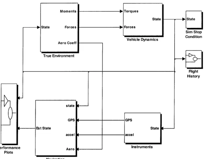
In order to provide a realistic testing environment for the navigation methods de-veloped in this thesis, a 6-DOF simulation environment was created using Simulink, with navigation algorithms implemented in Matlab. A top level view of the simulation environment is shown in Figure 2-1. Vehicle parameters for the simulation are based on a generic gun-launched projectile model developed at Draper Laboratory[2]. Sec-tion 2.1 describes the equaSec-tions of moSec-tion used in the simulaSec-tion, SecSec-tion 2.2 describes the atmospheric model, and Section 2.3 describes modelling of the aerodynamic forces on the vehicle.

2.1

Equations of Motion

The vehicle position, velocity, attitude, and angular rate are modelled in a 6-DOF simulation in Simulink using a flat earth gravitational model. The translational equa-tion of moequa-tion is

j1 = 91 + Lift + Drag (2.1)

The rotational equation of motion is

IWB = Moment + WB X IWB (2.2)

where lift, drag, and moment are vector valued quantities in the appropriate frames. Vehicle orientation is represented by an attitude quaternion in simulation, which is propagated using

0 Wz -Wy WX

-WY 0 ox Yq _(2-3)

where the scalar component of q is in the last term.

Physical property values for the projectile model, plus nominal launch conditions, are provided in Tables 2.1 and 2.2. An example of a typical vehicle trajectory is shown in Figure 2-2.

GPS GPS

State State

accel

Aero Instruments

Navigation

Table 2.1: Nominal launch conditions

Launch Elevation 45 deg

Launch Velocity 550 m/s

Roll Rate (w.) 2 Hz

Table 2.2: Vehicle properties

Mass (m) 30 kg

Moment of Inertia (Ix) 0.054 kg - m2

Moment of Inertia (IT) 0.252 kg - m2

Radius 0.06 m

Length 0.3 m

2.2

Atmospheric Model

The atmospheric density used to calculate aerodynamic forces on the vehicle body is approximated by a simple adiabatic model of the atmosphere. While this method is less accurate than using tabulated atmospheric data, it has the advantage of run-ning significantly faster than a table lookup when implemented in the Simulink en-vironment, and does not vary markedly from tabular data at the altitudes involved. Assumed atmospheric conditions at sea level are shown in Table 2.3.

The temperature at altitude h is

T _ gh

TO-

1 RT

where To is the surface air temperature. The air pressure at altitude h is

(2.5)

where Po is the surface pressure. The air density is then just P

RT

PO

RTo

2.3

Aerodynamic Forces

Aerodynamic coefficients are based on a generic projectile model developed at Draper. Lift, drag, and pitching coefficients are modelled as functions of Mach number (A) and angle of attack (a-) in degrees. These values are included as Table 2.4.

P

-y gh ]

0) C

0 10 20 30 40

Time (sec)

50 60

Figure 2-2: Typical vehicle trajectory

Table 2.3: Atmospheric conditions Surface Air Temperature (To) 298.16 K

Surface Air Pressure (Po) 1.013e5 N/m 2

Gas Constant (R) 287 J/kg/K

Specific Heat Ratio (y) 1.4

The dynamic pressure can be defined as

1

g0 = -pIvI 2

2

(2.8)

where p is the atmospheric density found in 2.6. Taking velocities in the body frame,

the transverse component of velocity can be written as

Vt =

[ 0

and the angle of attack defined as

o= sin-1 |Vt| |VBI

22

(2.9)

(2.10)

Table 2.4: Aerodynamic coefficients

Reference Area (Aref) 0.0113 m2

Reference Length (Lref) 0.3 m

Cm --0.028290 Ma -0.00196 M +0.16126 a +0.00127 Cdo 0 Ma 0 M -0.13650 a +0.74235 Cda 0

Defining the additional unit vectors

in Vt

. [0 +iZn -in, ]T

[0 +in -in, ]T|

i= [1 0 0 ]T

the moment, lift force, and drag force of 2.1 and 2.1 can be defined as

Lift = ArefCmaq.in

Drag = -Aref (Cd₀ + Cdna 2_{) qix}

Moment = ArefLefCaqooi, (2.11) (2.12)

(2.13)

Chapter 3

Measurement Transformations

As discussed in Chapter 1, the elimination of gyros in the navigation system of a gun-launched projectile would have significant advantages in terms of cost and launch reliability. In order for gyro-free navigation to succeed, a method of estimating an-gular rates using only accelerometer outputs must be developed. This is possible in a spinning projectile because the outputs of the accelerometers will have components due to both centripetal and Euler accelerations in the body-fixed reference frame.

This chapter defines the relationships between the motion of a general rotating body and the outputs of accelerometers fixed to the rotating frame of reference. Section 3.1 is based on previous work by Asher [1], and derives the relationships between vehicle state and accelerometer outputs, and shows them to be linear functions of the vehicle linear acceleration, angular acceleration, and rate products of the form w and wiwj. Section 3.2 describes a deterministic method of recovering the angular rate from the accelerometer outputs in the case of error-free sensors. This method is greatly improved upon by the Kalman filtering method to be presented in Chapter 4. Finally, Section 3.3 presents the nominal configuration of 12 accelerometers used throughout the remainder of the thesis.

3.1

Accelerometer Outputs

The acceleration of a point ri within a rotating reference frame is

ai = SB

+aB

+ wB

where SB is the acceleration resulting from the body specific force vector at the origin of the coordinate system, CB is the angular acceleration, and WB is the angular rate. The output of an accelerometer at this point with sensitive axis aligned along the unit orientation vector

ei

fi

'The matrix form of the cross product is used throughout. Expressions such as [a x] are equivalent

0 -az ay

to the 3 x 3 matrix of vector components a 0 -a, The expressions a x b and [ax]b

-aa a 0_

The final term in (3.2) contains the centripetal acceleration, which can alternatively be written in matrix form as

WY WI _W2 2 X z WYWZ 2 21 (3.3) [wLBX] [WOBX] LL wyw W1W1

~

This gives six different rate products, representing both square and cross product terms. These terms can be represented by a symmetric matrix W of rate products, so that (3.3) can be rewritten as

W1 1 [W BXHWBXI= W12 W₁₃ W12 W₂₂ 11/23 V13 W23 W33 (3.4)

Using this expression for W, and rewriting (3.2) in matrix form gives

fi

O

where w, represents the vector of cross term components the square terms. The full set of accelerometer outputs matrix form as o . n T W12 W13 WV23 Win W 2 2 'V3 3 = [ mT

[

f i

f.

-of

{rix}

-f

nT_{1l SB I} . T nT . S n or more compactly as

f

Using a set of at least twelve accelerometers, and assuming no instrument or errors, the body forces, angular accelerations, and rate products W can be directly by taking the pseudo-inverse of M in (3.8), giving

r = M#f = Ef (3.7) (3.8) biases found (3.9) 26

where the pseudo-inverse M# is used to allow for the case of more than 12 accelerom-eters. This gives the specific force, angular acceleration, and rate products as linear functions of the accelerometer outputs. Selected components of the vector rq can then be calculated through appropriate partitioning of the matrix E.

SB Ei

K

=.. E2

f

Wc E3

sJ E4 J

3.2

Deterministic Solution for Angular Rates

It is possible in principle to determine the angular rate components directly from the sensor outputs if the accelerometers are assumed to be error-free. One way of accomplishing this is to note that the vector triple product

[WBX][WBX]WB = WOB (3.11)

should always be zero, since it is the orthogonal projection of the rate vector oB onto itself. Using the estimates for the rate products found in (3.9) to construct W, the direction of the rate vector can be found by looking for an eigenvector with a corresponding eigenvalue of 0. The magnitude of the rate vector can also be found by evaluating the trace of W, giving

tr[W] = -2 [w2 + W2 + W] (3.12)

1WBI t

V/-tr [W}

2

The sign ambiguity in (3.13) can be resolved by recognizing that for a spinning projectile, the sign of the angular rate about the spin axis is known, e.g. W > 0.

Using this fact, and assuming an eigenvector of the form

e=[1 ey ezT (3.14)

The product We can be rewritten as

W1 2 W13 -Wu

1

W22 W2[3 1 e - W12 (3.15)

W23 W33 _ j

L

J

Since the terms W22 and TV3 3 contain -wi, their product should always be positive.

Taking the last two equations, the components of e can be found using

-W/V1 2 WV3 3 + WV1 3 2 3

Table 3.1: Accelerometer configuration Position Orientation Accel# x y z x y z 1 +d 0 0 0 0 +1 2 +d 0 0 0 +1 0 3 -d 0 0 0 +1 0 4 0 +d 0 +1 0 0 5 0 +d 0 0 0 +1 6 0 -d 0 0 0 +1 7 0 0 +d 0 +1 0 8 0 0 +d +1 0 0 9 0 0 -d +1 0 0 10 -d 0 0 +1 0 0 11 0 -d 0 0 +1 0 12 0 0 -d 0 0 +1 --W1 3W2 2 + W1 2W2 3 e-=(3.17) 2+W22W33 - W13W23

The rate vector is then

i+/-tr [W] e

WB = -- (3-18)

2

je

l

with the sign determined by comparison to the known spin direction of the vehicle. An alternate method of resolving the sign ambiguity in (3.18) is to make use of

the angular acceleration information in E2

f.

successive updates with the angular acceleration would allow sign determination, but special care would need to be taken to properly account for sensor noise.

In practice, a deterministic solution for the rates is not practical, given the large biases and noise levels expected. Chapter 4 introduces a better Kalman filter based method of solving for rates in a noisy environment.

3.3

Instrument Configuration

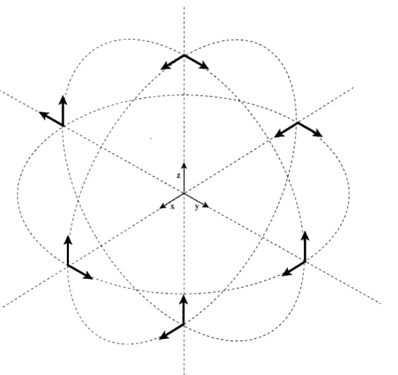
For all subsequent work, the 12 instrument configuration proposed in [1] is used. This configuration places the instruments in orthogonal pairs on the faces of a cube, with one instrument from each pair of opposing sides facing radially outward from the center. A diagram of this arrangement is presented in figure (3-1). All instruments

are equidistant from the cube center, with nominal displacement d = 5 cm. Table

(3.1) gives the position and orientation of each sensor.

4.

z

IA - A

/A XI Y

(A . - - /

Figure 3-1: Accelerometer configuration

4

t

I

Chapter 4

Filter Implementation

Chapter 3 showed that an accelerometer-only navigation system can provide measure-ments of angular acceleration, which can then be integrated to provide an estimate of the angular rate. Linear combinations of the accelerometer outputs were also shown to provide measurements of angular rate products of the form W and wiwj. It would be useful to develop a navigation filter that could use these additional measurements to help stabilize the integration of the angular rate, as well as to incorporate GPS measurements as they become available.

This chapter develops the 24-state Kalman filter used throughout the thesis. The filter includes 3 element states for perturbations in position, velocity, orientation, and angular rate, as well as 12 states for the accelerometer biases.

Section 4.1 presents the standard set of Kalman filter equations required by the navigation algorithm. Section 4.2 derives the linearized state equations used in the filter. The angular rate is included in this section as a state, since no direct measure-ment is available. The section concludes with a brief discussion of the possibility of accounting for sensor misalignments through bias estimation.

Section 4.3 describes how GPS measurements and measurements of the angular rate products w and wow are handled by the navigation filter. Since rate products are non-linear functions of the rate, measurement partials calculated in this section require the use of an extended Kalman filter. Position and velocity estimates from a pre-computed firing solution may provide a substitute in the absence of GPS prior to signal acquisition.

Section 4.4 describes how navigation system states are propagated and updated based on perturbation states calculated in the Kalman filter. While the attitude perturbation state is represented as a vector in 4.2, the total attitude estimate is characterized here in quaternion form, giving a 13 element vector for the reference state.

Section 4.5 describes the pitfalls of using a linearized filter for rate estimation. Techniques for reducing some of the errors characteristic of an extended Kalman filter during initialization are suggested.

4.1

Kalman Filter Equations

The Kalman filter is a recursive estimation algorithm devised by R.E. Kalman in 1960

[7], a derivation of which can be found, for example, in [3]. Since a spinning projectile

has non-linear equations of motion, an extended Kalman filter formulation is used, where the filter states represent small perturbations 6x of the vehicle state about its nominal value :-. After each Kalman filter measurement update, the filter states are

applied as corrections to the reference state, and are then reset to zero.

Using the discrete form of the filter, a small perturbation 6x about the nominal trajectory evolves according to the state transition equation

SXk = kPOXk_1 + Wk (4.1)

where D is the state transition matrix, and Wk is a process noise term with covariance given by

Qk = E[wkw ] (4.2)

Estimates of the state perturbation before and after the kth measurement is in-cluded are written as Si and &i:, respectively, and are updated between measure-ments using the state transition equation

65ik = 4)k&Xk (4.3)

The covariance of the estimation error is given by

Pk = E[(6Xk - Xk)(6Xk - Sek)]

(4.4)

and is updated between time steps using the covariance transition equation

Pk = _kPkim + k (4.5)

The measurement error Vk is defined as the difference between the actual

measure-ment Zk, and the estimated measurement .k

Vk = Zk -- k (4.6)

Vk = Zk - C0oCk

(4.7)

The covariance of the measurement error is

Rk = E[(zk - Zk)(Zk - Zk)T]

(4.8)

Since the filter state estimates

oc

After obtaining the kth measurement, the estimated state is updated using

ok+

where the Kalman gain matrix Kk in (4.9) is defined as

K.

P

(

C

R,)-

(4.10)

The covariance matrix is also updated using the Kalman gain matrix,

P+ = (I -

)P_

(4.11)

4.2

State Transition Equations

The equations of state for a general rotating body can be written as

dr = o _(4.12) dt dv1 = AIBSB +g ₁

_(4.13)

dt

_(4.14)

dt

=

_(4.15)

where rj is the inertial position of the body, v is the velocity, SB is the acceleration from specific force in the body-fixed reference frame, WB is the angular rate of the body frame, aB is the angular acceleration, and the matrix AIB is a 3 x 3 rotation matrix from the body to the inertial frame. The reverse rotation can be obtained using

A-'

A TB

(4.16)

since AIB is orthonormal.

Note that in (4.15), WB has been included as a state. This is unusual in an inertial navigation problem, where typically the body rate is taken directly from gyro mea-surements. In the accelerometer-only case, no direct rate measurement is available, so the rate must be estimated along with the other states.

The states x in (4.12-4.15) are treated as having small perturbations about a reference state :-, so that r, = r, + 6r1 , with equivalent expressions for the velocity,

v1, and angular rate, WB. The attitude is written as the product of the reference

attitude AIB and a small rotation

N/B

AIB = AIB(I±[OBX])

(4.17)

This can be rewritten in terms of the reference attitude by recognizing that

AIB AIB(I + [B XD-- (4.18)

~ AIB(I + [PB X)) (4.19)

4.2.1

Position Perturbation State

The differential equation for position can be written as

d(ri +

orj)

dt

Substituting for vI and differentiating,

+ d, = ;-I + 6vI (4.22)

dt

leaves the desired equation for the position perturbation,

d(6r

)

8vi

dt

4.2.2

Velocity Perturbation State

The equation for velocity is written as

d(i

+ 6v

) _

_(4.24)

dt

Differentiating and expanding the right hand side results ini

d(Jvi)

AIB5B

+

-51

+

=

d(JvI)

dt

=

(4.26)

SB comes from the specific force perturbation. Taking only first order terms and rearranging slightly leaves the equation for the velocity perturbation,

d(ov1)

di = -AIB[ BXI1B + AIBESB (4.27)

4.2.3

Attitude Perturbation State

From (4.14), the differential equation for the attitude is

dAIB = AIR[WBX]

(4.28)

dt

which can be compared to the result obtained from direct differentiation,

dAIB _ d(AIB{JI+[V)BX _(4.29)

dt

dt

'It is assumed here that the gravity term gr is constant, so that 6g, = 0, or g, = 91

The right hand side of the first equation can be expanded to include perturbation terms:

dAI

dIB - AIB(J + [BXD([OBX] + [WBX]) (4.30)

dt

Differentiating the second equation,

d AIB - d'@P

d =AIB B X + AIB[CBX(I + BBX])

(4.31)

dt dt

and combining the two gives

(I

(4.32)

Taking only first order terms leaves

[OBXI(QBX1 + [WBX) = [dIB

_dt

This can be further reduced by noting the matrix identity

[COBXI[lPBX] - [BXI[CBX] = [(OB X IB)X]

(4.34)

Applying the identity and converting to vector form gives the desired equation for

the attitude perturbation2

d@B - _{FBXPPB +} 6

WB _(4.35)

dt

4.2.4

Rate Perturbation State

The differential equation for the angular rate is

d(CB + SWB)= aB _(4.36)

dt

Differentiating and expanding the right hand side

- d(6wB)

-tB

+ = 5B + SaB (4.37)

dt

leaves the desired equation for the rate perturbation

d(JwB) =

JaB

_(4.38)

dt

2

Attitude perturbations in inertial navigation are more often expressed in the inertial frame

AIB = J+[ Pix)AIB

which, after similar manipulation, results in a dynamical equation of the form

dt

The choice of the body-frame representation chosen here will become apparent in Section 5.3, where

4.2.5

Instrument Errors

Perturbations of the specific force and angular acceleration vectors required in (4.27) and (4.38) can be written as functions of the accelerometer outputs,

oSB =

E

aB E26f(4.39)

where E1 and E2 are the matrix partitions introduced in (3.10), and

of

6f = 6f+V (4.40)

The perturbation in (4.40) is the uncompensated accelerometer measurement bias 6,3 plus a noise process vf. This noise process can be modelled as the sum of quan-tization errors and a white noise process. Quanquan-tization errors are assumed to be uniformly distributed over the quantization interval q. For an accelerometer with n bit output over a range of ±a, the measurement error due to quantization over the

range ±/2 can be characterized by

a

-,=

2n

(4.41)

where the quantization interval q is given by 2a

q = 2a (4.42)

Assuming an additional random walk term orw, the covariance matrix for the

ac-celerometer outputs

Qf

Q

=

+ O)I

(4.43)

Combining the filter state equations, the state transition equation can be written in matrix form as

~r

0 1

0

0

[

0

[V~

d

ov1

XIB[§BX1

bB = 0 0 -- WBXI 1 0B + 0

vf +

(4.44)

LW

d(Sx)

Fox +

where v, has been included as an optional additional white noise process for each of the filter states. Since the process noise in (4.45) has zero mean, the state transition equation (4.3) can be approximated by

4 = eFAt (I + FAt) (4.46)

6Sk = (%kSgk_1

(4.47)

The covariance propagation equation of (4.5) becomes

P= <k ki + QE ± Qs (-.4)

where the covariance noise matrix Qk has be separated into two components. The first is an effect of the accelerometer sensors noise:

Qf

EAQfE

and the second comes from the additional process noise term vs:

QS

4.2.6

Effect of Sensor Misalignments

An important error source not explicitly modelled in the filter is the effect of sen-sor misalignments. A misalignment in an accelerometer which is nominally aligned with the vehicle spin axis will experience a very large unmodelled disturbance due to centripetal acceleration effects. The following calculation shows how this error may be partially mitigated through bias estimation. Taking the instrument output transformation (3.6), the output of a given accelerometer is

fi

T

Defining the matrix permutations of the position vector ri

r i2 ril 0 ril 0 0

Rm

ri]

ri2

0

(4.52)

0

the accelerometer output may be rewritten as 67

SB -

6[ri

= OT(sB - [rix cB + RWc + Rn s) (4.54)

Define now a small misalignment Ai of the orientation vector 6,, so that

6,

=

(I+ [Ai x])Oi

(4.55)

The output error resulting from this misalignment is

sB

ri=

-

[Aix] [ I -(rix] RT

]

This can be greatly simplified if it can be assumed that terms resulting from lateral forces, accelerations, and rates will approximately cancel over a single revolution, the

angular acceleration about the spin axis is small, and that w, is dominated by the W term. In an average sense, the error resulting from sensor misalignment is roughly

(rs) ~ -O[9Xi x 0 + Rn -ofX (4.57)

0 -o _

This expression looks much like a bias, particularly in situations with high spin rates and low drag. The effect of misalignment on rate estimation, and the effectiveness of bias state compensation, is discussed in Section 6.1.3.

4.3

Measurement Equations

The state transition equations defined in (4.44) for the perturbation states use ac-celerometer outputs for calculation of the specific force vector SB and the angular acceleration aB. Additional information can be obtained about the angular rates by considering the measured values of the rate products defined in (3.10). This gives two vector measurements which can be used as a check on the integration of aB.

Additionally, data from an external source such as GPS may be available for state estimation. These measurements have a direct use in estimating the vehicle position and velocity, and also provide an indirect means of estimating vehicle orientation. In the absence of GPS, trajectory information from a pre-computed fire-control solution can be substituted to aide in the dynamics-based navigation measurements presented in Chapter 5.

4.3.1

Rate Measurements

The rate products in (3.10) can be used as measurements by taking the difference between these values and the products of the reference rates in the navigation filter. In the following, these measurements are represented as two different vectors, one with the rate cross terms, the other with the square terms. Beginning with the cross rate terms, the measurement can be constructed as

z = E3f - CUwz (4.58)

This can be rewritten in terms of the rate perturbation SOB and the uncompensated

bias Jo3. Thus

(wX -

SWo)(wY

-

OwY)

1

zWC = E3(f - 6#) - (wx - S6w)(w - Soz) (4.59)

y(w - SWx)(wz - JWz)

Taking partials with respect to the filter states and keeping only first order terms gives, for the rate

C D(S= B = oz 0 W (4.60) 0 oW Wy

and for the instrument bias

COc - O" = -E3 (4.61)

o9(6))

Similarly, for the squared rate terms the measurement may be constructed as

z[ E4f - - 22 (4.62)

which may once again be rewritten in terms of the true rates and rate perturbations

(wY - 6WY) 2

+

1

zws

=

(wPz - 6ox)2 + (WY - 6WY)2

The partial derivative matrices for this measurement are, to first order

_z _ 0 wL y w z

C -= -2 w 0 wz (4.64)

(

_ozw.Y

for the rate, and

CO =

6"3

for the instrument bias. Note, however, that the matrices defined in (4.60) and (4.64) require the true rates WB. Since these are obviously not known to the filter, it must make due with its best estimate of the rates, CB.

The measurements can now be modelled as linear functions of the filter states

zWo ~ 00CB g + VWC~

(4.66)

z[,

1

where the measurement noise terms vwC and Ls come directly from the accelerometer

noise error v1 in (4.45). Thus

voc = E3Vf (4.67)

VWS

(4.68)

The two vector measurements are correlated, and the combined measurement noise matrix R required in (4.10) can be expressed as

4.3.2

GPS Measurement

If position and velocity measurements are available from GPS, or from an alternate

source such as a pre-launch firing solution, then the measurement vector can be augmented to include these terms. First, the position and velocity measurements are constructed in terms of the reference values:

z, = ry. - r1

(4.70)

zV = Vgps -fi- (4.71)

where rgps and vgp, are from GPS or similar measurements. Rewriting in terms of the perturbation states,

Zr = rp, - (r, -

6r

zV = v9,, - (v1 - Sv1) (4.73)

The partial derivatives with respect to the filter states are

asri)= I (4.74)

8(or1)

=

I

8(6v1)

The measurement model is

r1~

Z

1I 0 0

I

(4.

'' C'10 0 3P + V (4.76)

zV

0 1 0 0 0

-

and the measurement covariances for these two measurements are defined as

Rr

E[vvT]

RV

E[vvi]

Combining the measurement equations for all measurement types gives the total matrix of measurement partials C

0 0 0 CWc

COC~

C

0 0 0 C

CO

(4.79)

1 0 0

0

0

and matrix of measurement error covariance R

Rw

0

R

R

0

(4.80)

0 Ri required in (4.10) and (4.11).

4.4

State Update Equations

4.4.1

Propagating the Reference State

The state transition matrix defined in (4.46) is defined for the filter states. Before ap-plying the correction to the reference state found in the perturbation state calculation in (4.9), it is necessary to propagate the reference state to the next time step. This calculation is performed independently from and prior to the Kalman filter updates. The position, velocity, attitude quaternion, and angular rate can be defined as a 13 element state vector of the form

[Vi

(4.81)

q .WB_

The reference states can be propagated using the specific force and angular accel-eration terms defined in (3.9). The update equations for these states are

14i + ;I At (4.82)

bj 4= ;i1

+

+

(4-83)

WB - COB + 'BAt (4.84)

A very simple form for the attitude update takes the rate as a constant over the

integration interval. The attitude quaternion is written as a rotation from the inertial frame to the body frame. The quaternion is defined with vector part qv and scalar part q, such that q = [qv, qs], following the convention in [10] . For a short time step, the quaternion update can be approximated by

0

+ ~_A 0 U $D At q (4.85)

2 Dy -(DX 0 D2

The quaternion at the midpoint of the timestep At should be used to calculate the reference attitude AT required in (4.45) and (4.83). This can be found be replacing

At with A in (4.85). The 3 x 3 rotation matrix ATB can then be found by transforming

the quaternion to matrix form

ATB = (q2 -

qTqv)I +

(4.86)

4.4.2

Applying the Error States

Once the reference state has been propagated to the new time step, the filter states can be applied. Since state perturbations were defined as positive quantities in Section

4.2, the state corrections for position, velocity, angular rate, and bias are just

Y1 I ;1 + 601 (4.87)

I <= b1 + f';1 (4.88)

WB B

+

(4.89)

,8 <= ) + J,3 (4.90)

The attitude correction in matrix form comes from (4.17)

A

However, since the reference attitude attitude state is a quaternion, the correction must be made in this form. Defining the correction rotation as

4e~ ~ ('0,i1] (4.92)

the attitude correction becomes

4 < q -b (4.93)

where the quaternion multiplication operation is defined as

q1 -q2 = [(q1v x q2v + q2sq1

+

),

4.5

Managing Rate Linearization Error

Since the filter scheme proposed is an extended Kalman filter, stability of the rate estimate is not guaranteed, since calculation of measurement partials in (4.60) and (4.64) depends on the filter's own rate estimate. If the rate estimation error is large, the error in C will also be large, leading very quickly to filter divergence. This problem is particulary acute during filter initialization, since the initial rate may not be well known. The problem is most notable in cases with large initial biases, or large sensor noises.

As noted in [31, most proposed solutions to this problem are based on ad-hoc numer-ical tricks and are not easily generalized. In the current problem, several modifications to the filter can be made to help reduce the risk of divergence in the first few filter updates. These modifications will be referred to collectively as EKF compensation.

The first modification is to construct the C matrices of (4.60) and (4.64) based on a nominal rate Wnom, _{rather than the reference rate C'. This approximation helps to}

pre-vent a large transient estimation error from causing divergence. In the final form of the navigation filter, this approximation was made for the first 1/10 sec (10 filter steps), and was done only to the roll rate, since this is by far the largest rate component.

The second modification scales the measurement noise matrix by a constant factor k, also for the initial 1/10 sec. This modification causes the filter to make smaller initial rate corrections over the first few steps. This is necessary since the initial covariance matrix P- is relatively large, and the angular rate error might otherwise