Martin Hilpert* and David Correia Saavedra
Using token-based semantic vector spaces
for corpus-linguistic analyses: From practical
applications to tests of theoretical claims
https://doi.org/10.1515/cllt-2017-0009
Abstract: This paper presents token-based semantic vector spaces as a tool that can be applied in corpus-linguistic analyses such as word sense comparisons, comparisons of synonymous lexical items, and matching of concordance lines with a given text. We demonstrate how token-based semantic vector spaces are created, and we illustrate the kinds of result that can be obtained with this approach. Our main argument is that token-based semantic vector spaces are not only useful for practical corpus-linguistic applications but also for the investigation of theory-driven questions. We illustrate this point with a discus-sion of the asymmetric priming hypothesis (Jäger, Gerhard and Anette Rosenbach. 2008. Priming and unidirectional language change. Theoretical Linguistics 34(2). 85–113). The asymmetric priming hypothesis, which states that grammaticalizing constructions will be primed by their lexical sources but not vice versa, makes a number of empirically testable predictions. We oper-ationalize and test these predictions, concluding that token-based semantic vector spaces yield conclusions that are relevant for linguistic theory-building. Keywords: semantic vector spaces, token-based, word sense disambiguation, asymmetric priming
1 Introduction
This paper showcases token-based semantic vector spaces (Schütze 1998; Heylen et al. 2012, 2015) as a tool for corpus-linguistic analyses. More specifically, it is the aim of this paper to demonstrate how this technique can be applied to linguistic research questions that address theoretical claims. To this end, the paper will explain how the technique works, show how it can be used for several practical corpus-linguistic tasks, and discuss a case study in which it is put to
*Corresponding author: Martin Hilpert, Department of English, Université de Neuchâtel, Neuchâtel, Switzerland, E-mail: [email protected]
David Correia Saavedra, Department of English, Université de Neuchâtel, Neuchâtel, Switzerland
work in the context of an open question in grammaticalization theory, namely the asymmetric priming hypothesis (Jäger and Rosenbach 2008; Hilpert and Correia Saavedra 2016).
Semantic vector space models, of which token-based semantic vector spaces are a special subtype, are routinely used in computational linguistics, where they are applied to problems such as word sense disambiguation or information retrieval (Turney and Pantel 2010). The technique has been adopted by a number of corpus-based studies (e.g. Sagi et al. 2011; Jenset 2013; Perek 2016; among others), and it is featured in a recent corpus linguistics textbook (Levshina 2015), but overall, it remains an underused technique. Its core idea is captured by the slogan You shall know a word by the company it keeps (Firth 1957: 11), which reflects the hypothesis that the meaning of a word is directly related to its distribution in actual language use. Using a corpus of language use, it is possible to analyze the meaning of a given word in terms of other words that occur frequently in close proximity to that word. For instance, the noun toast frequently occurs in close proximity of nouns such as tea, cheese, slice, and coffee, that is, its typical collocates. A statistically processed frequency list of all collocates of toast in a given corpus is called a semantic vector. Semantic analysis enters the picture when semantic vectors of several words are com-pared. Two words are in a semantic relation if their semantic vectors are highly similar, as measured by a statistic such as the cosine (Turney and Pantel 2010: 160). For instance, near-synonyms such as cup and mug will have similar semantic vectors, but also converses such as doctor and patient and even antonyms such as hot and cold will converge in their respective collocational behaviors. If a large group of semantic vectors is analyzed with a dimension-reduction technique such as multidimensional scaling (Wheeler 2005), semantic relations between those words can be visualized in a two-dimensional graph where words with close semantic ties are positioned in close proximity whereas semantically unrelated words are placed further apart.
The present paper builds on the general logic of semantic vector space modeling, but adopts a more specific proposal from Heylen et al. (2012): Whereas most current applications of semantic vector space models analyze word types, thus averaging collocate frequencies over many occurrences of the same word, Heylen et al. present an approach that operates at the level of word tokens, thus capturing meaning differences between individual occurrences of the same word. The primary unit of data in such an approach is the concordance line, that is, a key word with a context window of several words to the left and several words to the right. By comparison, a type-based frequency vector that contains an aggregation of many usage events is of course much more informa-tive than a concordance line, which will typically contain just a small number of
words, many of which appear just once, or at best twice. How can concordance lines be a reliable basis for semantic comparisons? In order to overcome the data sparsity that comes with the use of concordance lines, the method that Heylen et al. (2012) propose uses not only the direct collocates of the target word but also second-order collocates, that is, the collocates of all items that are found in a given concordance line. Heylen et al. use this technique, which will be explained in more detail in Sections 2 and 3 below, to analyze polysemous Dutch nouns. For instance, the noun monitor can mean‘computer screen’ as well as‘supervisor’. Heylen et al. compared different uses of monitor in terms of their second-order collocates and showed that the statistical method can fairly reliably differentiate tokens with the meanings ‘computer screen’ and ‘super-visor’. They present this analysis with a broader linguistic aim in mind. A visualization of different uses of a word can guide lexicographers in their task to identify different word senses with typical collocates. Similarly, the present paper argues that token-based semantic vector spaces can be used in linguistic work that is concerned with theory-driven hypotheses. The final part of this paper gives an illustration of this by using token-based semantic vector spaces to test a prediction of a hypothesis that concerns priming and semantic change. Jäger and Rosenbach (2008) have put forward the so-called asymmetric priming hypothesis, which predicts that grammaticalized forms (such as be going to) are primed by their lexical sources (the motion verb go), but not vice versa. Hilpert and Correia Saavedra (2016) have tested this prediction in an experimental setting, but did not find behavioral evidence to support the hypothesis. This paper provides an additional perspective on the problem by bringing corpus-linguistic data to bear on the issue.
The remainder of this paper is structured as follows. Section 2 starts by introducing the reader to the basic form of semantic vector spaces, which are constructed out of aggregated collocate frequencies of word types. As such a type-based semantic vector space constitutes the basis for the subsequent inves-tigations in this paper, the section walks the reader through the steps of how a type-based semantic vector space is created. Section 3 explains how token-based semantic vector spaces are constructed by matching the words found in con-cordance lines with frequency vectors from a type-based semantic vector space. The section presents three practical applications of this approach, namely the comparison of semantically related words, the discrimination of word senses, and the matching of a concordance line with the text from which it originates. Section 4 moves on to a discussion of how token-based semantic vector spaces can support hypothesis-testing in theoretical linguistic research, using the asym-metric priming hypothesis as an example. Section 5 concludes the paper by pointing out possible avenues for future research.
2 Construction of a type-based sematic vector
space
This section describes the construction of a type-based semantic vector space that forms the basis for the subsequent analyses.1A comprehensive description
of the approach is found in Turney and Pantel (2010), Levshina (2015) offers a useful introduction. The approach involves a series of choices that the analyst has to make, including the choice of a corpus, the size of the vocabulary that is included, how to select stop words that are automatically disregarded, how to measure similarity between vectors, and several others. Kiela and Clark (2014) present an overview of these choices and how they influence the results. In our case, the type-based semantic vector space represents a vocabulary of about 20,000 lexical elements and their co-occurrence frequencies with each other. The corpus that is used for this purpose is the 100-million-word British National Corpus (Leech 1992). In practical terms, the semantic vector space is a large table in which the column labels are the 20,000 vocabulary elements and the row labels are context items that co-occur with any of these vocabulary elements. The cells of the table are filled with values that indicate collocational strength between a vocabulary element and a given context item.
1. The first step of the process is the creation of a frequency list of all tagged elements in the British National Corpus. Of that list, the top 200 elements, which contain highly frequent types such as punctuation, articles (the, an), pronouns (he, them), and clitics (‘ll), are discarded. From the rest of the list, elements 201 to 20,200 are retained for further processing. The choice of 20,000 elements as our vocabulary size is meant to achieve a compromise between maximal cover-age and feasible computational effort.
2. The resulting list of 20,000 types is stripped of elements that represent punctuation, single-letter lexemes, numbers, forms of the grammatical verbs be, have, and do, and elements that are tagged as unclear. The reduced list consists of 19,429 types. Ordered alphabetically, the list starts with <w aj0-av0>above and<w aj0-av0>alike, and it ends with <w xx0>nt.
3. In order to minimize computational effort in the subsequent steps, a reduced version of the British National Corpus is created. All elements that are not contained in the list of 19,429 types are automatically discarded from the corpus. This procedure yields a corpus with 39.5 million tokens.
1 The data structures that are discussed in the following and the R code that has been used to create them are available from the authors upon request.
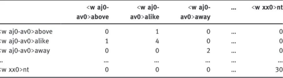
4. An empty data frame with 19,429 rows and 19<429 columns is created. The information that the data frame is meant to contain is how often each of the types co-occurs with each other in corpus data. The columns represent the 19,429 types of the word list. The rows represent the same elements in their function as context items. This means that the first column would hold informa-tion about the element <w aj0-av0>above, indicating how often it occurs with itself, how often with <w aj0-av0>alike, <w aj0-av0>away, and all other remain-ing elements, yieldremain-ing a vector of 19,429 frequency values. Table 1 illustrates the structure of the data frame.
5. In the next step, all cells of the data frame are filled with frequency values, proceeding column by column. In order to do that, concordance searches are performed for each column label, starting with <w aj0-av0>above, and continu-ing with <w aj0-av0>alike, <w aj0-av0>away, and so on. For these concor-dances, the reduced version of the BNC (cf. step 3) is used. Concordance lines consist of two elements to the left of the search term and two elements to the right of the search term, but not the search term itself. To illustrate, the element <w aj0-av0>above occurs 621 times in the reduced BNC. Using a context window of two left and two right, the concordance yields 4 x 621 = 2,484 context items in total. In these context items, the element <w aj0-av0>above itself is not found at all, which means that the first cell is filled with a zero. By contrast, the element <w aj0-av0>alike is found once, so that the number 1 is entered in the second row of the first column. Table 2 shows the co-occurrence frequencies that are determined for all types and context items that are shown.
What can be seen is that there is a tendency for elements to occur with themselves. The element <w aj0-av0>alike has itself as a context item 4 times (out of 4,400 context items); the element <w xx0>nt occurs 30 times with itself (out of 1,468 context items). With all cells in the data frame filled out, each element in the column labels is now represented by a vector of 19,429 frequency values.
Table 1: Data frame for co-occurrence frequencies.
<w aj-av>above <w aj-av>alike <w aj-av>away … <w xx>nt <w aj-av>above <w aj-av>alike <w aj-av>away … <w xx>nt
6. The sixth step is the transformation of the token frequencies in Table 2. The purpose of having co-occurrence frequencies arranged in the format of Table 2 is that elements can be compared in terms of how similar their respective frequency vectors are. Similar frequency vectors, so the argument goes, will be a reflection of semantic similarity between elements. However, there is a basic problem. Comparisons of raw token frequencies, as shown in Table 2, will not be reliable. Elements that are relatively infrequent will by necessity have many cells in common in which there are zeros, and even those cells that are populated with positive token frequencies will not differ dramatically. As a result, their mutual similarity will be overestimated by statistical distance measures. In order to solve this problem, the frequencies in Table 2 are transformed using the association measure of Pointwise Mutual Information (PMI), which is shown in (1).
(1) PMI = ln---pðx, yÞ
pðxÞ * pðyÞ
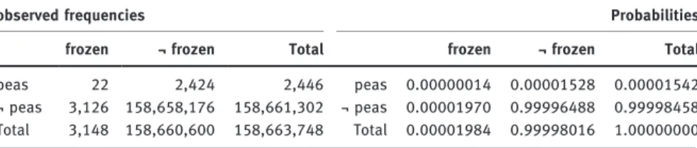
The PMI value of a pair such as frozen and peas is computed as the natural logarithm of the joint probability of frozen and peas (p(x,y)), divided by the product of the individual probabilities of frozen (p(x)) and peas (p(y)). These probabilities can be computed on the basis of the observed frequencies of frozen, of peas, the frequency of their occurrence, and the number of all observed co-occurrences in the corpus that is being used. In our case, the number that represents the totality of all observed co-occurrences equals the sum total of the frequencies that are contained in Table 2. An illustration of the observed co-occurrence frequencies of frozen and peas is given in Table 3.
As the left panel of Table 3 indicates, frozen and peas co-occur 22 times in our database. The element frozen occurs in 3,148 combinations in total, peas occurs in 2,446 combinations in total. The right panel of Table 3 shows the
Table 2: Filled-out data frame for co-occurrence frequencies.
<w aj-av>above <w aj-av>alike <w aj-av>away … <w xx>nt <w aj-av>above … <w aj-av>alike … <w aj-av>away … … … … … <w xx>nt …
respective probabilities of finding either frozen peas, frozen, or peas, if one of the 158 million word combinations of Table 2 is drawn at random. If these prob-abilities are entered into the formula given in (1) above, a PMI value of 6.13 results for the combination of frozen and peas, indicating that the two words are mutually attracted.
(2) PMI = ln 0.00000014
---0.00001984 * 0.00001542 = 6.13
In practical terms, the sixth step is the application of PMI to all cells in Table 2, which leads to the result that is shown in Table 4. In that table, each column label is represented by a vector of 19,429 PMI values that are comparable to one another.
7. In the interest of minimizing the computational effort of the subsequent analyses, this step reduces the size of the data frame of PMI values that was created in the most recent step. In practical terms, every column in the table adds a vocabulary item that can be of use in a future analysis, and every row in the table adds a context item that can potentially help to discriminate between
Table 3: Joint and individual frequencies and probabilities of frozen and peas.
observed frequencies Probabilities frozen ¬ frozen Total frozen ¬ frozen Total peas , , peas . . . ¬ peas , ,, ,, ¬ peas . . . Total , ,, ,, Total . . .
Table 4: Co-occurrence frequencies transformed into PMI values.
<w aj-av>above <w aj-av>alike <w aj-av>away … <w xx>nt <w aj-av>above . … <w aj-av>alike . . … <w aj-av>away . …
… … … …
these vocabulary items. Columns that only contain fairly low PMI values are thus vocabulary items that can be dispensed with. Rows that consist only of low PMI values do not allow us to distinguish between vocabulary items, and so also these rows can be deleted. In order to retain only the most informative columns and rows, an arbitrary cut-off point of PMI = 5.5 was selected. All columns and rows without a single value in excess of 5.5 were thus deleted, which diminished the size of the data frame to 12,621 vocabulary items by 12,619 context elements. The results of the seven steps discussed above are displayed in Table 5, which shows the top ten context items in terms of PMI values for three different vocabulary elements. For the elements <w aj0>frozen, <w nn1>syntax, and <w vvb>eat, the context items with the highest PMI values clearly show different semantic relations.
With <w aj0>frozen, the context items with the highest PMI values include food items that are typically frozen (peas, cod, turkey, etc.), and context items such as cooked or freezer are metonymically related to the frame of handling frozen food. The vocabulary element <w nn1>syntax has context items that relate to both linguistics and programming, which reflects its polysemy. Items such as seman-tics, vocabulary, and lexicon point to the linguistic sense of syntax; items such as identifier, invalid, and error point to its computational sense. Finally, the voca-bulary item <w vvb>eat is associated not only with food items but also with verbs that belong to the semantic frame of eating, i.e. cook and drink etc.
Basically, the data frame that was created in steps 1-7 is thus nothing more than a repository of words in which each word is associated with a long list of collocates and the corresponding PMI values. Creating such a list for any one
Table 5: Top ten PMI values of the context items of three vocabulary elements.
<w aj>frozen <w nn>syntax <w vvb>eat
context item PMI context item PMI context item PMI <w nn>peas . <w nn>semantics . <w vvb>eat . <w nn>cod . <w nn>syntax . <w nn-vvb>drink . <w nn>wastes . <w aj-nn>vocabulary . <w vvb>drink . <w nn>foods . <w nn>identifier . <w nn-vvb>sleep . <w vvn>cooked . <w aj>invalid . <w nn>calories . <w aj>frozen . <w nn>lexicon . <w nn>carrot . <w nn>packs . <w nn>error . <w nn>cake . <w nn>freezer . <w nn>punctuation . <w nn>foods . <w nn>turkey . <w vvb>supply . <w vvb>cook . <w nn>pellets . <w aj>semantic . <w nn>custard .
word, e.g. for the adjective frozen, is not a big challenge and can easily be replicated with online corpus interfaces, such as Mark Davies’ BYU-BNC (Davies 2004). However, we will explain below that having a type-based semantic vector space, that is, a collection in which several thousands of context vectors are pre-compiled and readily available allows for types of corpus analysis that would be difficult to achieve with an approach in which such vectors are created indivi-dually and ad hoc. The next section presents how we make use of our database for the creation of token-based semantic vector spaces, which allow us to compare individual concordance lines.
3 Practical analyses with token-based semantic
vector spaces
As was discussed in the introduction, most current applications of semantic vector spaces represent word types in databases of the kind that was described in Section 2. Such databases can be used to study semantic relations between word types, in particular degrees of synonymy or co-hyponymy. For instance, the type-based semantic vector space that was discussed above reveals that nouns such as cow, sheep, and pig occur with similar sets of context items. This section moves on to token-based semantic vector spaces (Heylen et al. 2012), which extend the approach in such a way that it allows comparisons at the level of individual usage events. This section presents three kinds of prac-tical analysis that can be done with token-based semantic vector spaces, namely token-based comparisons between different lexical elements, token-based com-parisons between different word senses, and concordance-line based compar-isons between different texts. Importantly, these analysis types draw on the database that was discussed in the last section, but they involve additional analytical steps that will be discussed below.
3.1 Distinguishing tokens of lexical elements on the basis
of their contexts
It is a basic tenet of distributional semantics that the meaning of a word is reflected in the items that are found in the immediate surroundings of that word. For example, the following five concordance lines of the key word fish, taken from the BNC, include many contextual items that serve as reliable cues to the key word.
(3) 1 fish and chips, I fancy fish and chips. No you don’t 2 ancient Chinese process is a fish preserving method comparable 3 hot dogs Wednesday, battered fish Thursday and turkey jackets on 4 herring guts was made into fish meal. That was in the field as 5 call them. What’s raw fish? Salmon. Disgusting. Pukey The left and right contexts in these five concordance lines are so strongly predictive that a speaker of English would be able to identify fish as the correct key word rather easily. An interesting aspect of this ability is that while all the contexts point to the key word fish, they do so with different cues. In fact, the contexts in the different concordance lines do not share any of their lexical elements. This leads to an interesting conceptual problem when the concor-dance lines in (3) are compared to five concorconcor-dance lines of another key word, namely the noun wish, in (4).
(4) 6 with great sorrow, the wish of the divorced Charles 7 authority or Toby Knight’s wish for a permissible framework to 8 to me and had no wish to cause me embarrassment 9 frustration and anger and a wish to do bad things; to hurt 10 see the reasoning behind your wish to introduce air into the
To a human observer, it is immediately obvious that the contexts in lines 3 and 4 above, even when the key word is disregarded, are semantically quite similar, whereas the contexts in line 3 and line 8 would be very different. Yet, a naïve computational comparison of the two pairs, based on a simple count of over-lapping lexical items, would yield the counterintuitive result that 3 and 8 are actually more similar. As is shown in (5) below, lines 3 and 4 do not share a single contextual element. Lines 3 and 8 share at least the word and.
(5) 3 and, battered, dogs, hot, jackets, on, Thursday, turkey, Wednesday 4 guts, herring, in, into, made, meal, That, the, was, was
3 and, battered, dogs, hot, jackets, on, Thursday, turkey, Wednesday 8 and, cause, embarrassment, had, me, me, no, to, to
Semantic vector space models typically exclude highly frequent words such as and, but this does not resolve the issue. Even if function words are discarded as elements that should not be counted in comparisons of this kind, the fact remains that a simple count of overlapping words cannot capture the strong
intuition that 3 and 4 convey roughly similar meanings while 3 and 8 do not. Importantly, intuitions of semantic similarity are not only based on the exact words that are found in an utterance but crucially also on the associations that these words evoke. In other words, concordance lines 3 and 4 may well consist of completely different words, but the associations of these words converge to overlapping sets of ideas. By contrast, the words in concordance lines 3 and 8 evoke completely different associations.
The type-based semantic vector space described in the previous section can be exploited for comparisons of concordance lines that do not only draw on the words that are actually present in those concordance lines, but that work on the basis of the typical collocates of those words, that is, the so-called second-order collocates of the key word. To take a concrete example, concordance line 3 of the key word fish contains the word battered. If we look up the collocates of battered with the highest PMI values in our database, the noun cod is among the highest-ranking elements. This makes cod a second-order collocate of fish. Similarly, the word herring in concordance line 4 has cod as one of its top collocates. So while concordance lines 3 and 4 do not have any of their actual words in common, their respective context items point to the same second-order collocates, which makes the concordance lines similar to one another. Drawing on the vocabulary items that are contained in our type-based semantic vector space, a concordance line can be represented by a vector that combines and averages over the PMI values of the second-order collocates of all words that are contained in that concor-dance line. We can exemplify this idea with concorconcor-dance line 5, which is repeated here for convenience:
(6) 5 call them. What’s raw fish? Salmon. Disgusting. Pukey
Of the words that are present in the left and right context, the words raw, salmon, and disgusting are contained in our database. These words are asso-ciated with the elements that are shown in Table 6.
Taken together, the context items that are listed in Table 6 and their PMI values form a semantic representation of concordance line 5. That represen-tation is richer than the words raw, salmon, and disgusting as such, because it also includes words that are commonly associated with these items. At the same time, it is clear that a semantic representation that is based on three words and their collocates is still impoverished when compared to the actual idea that a human speaker might form upon hearing concordance line 5. Still, the table illustrates that a single word with strong associations to the key
word fish is able to evoke a whole range of closely related concepts. If this logic is applied to a set of concordance lines of the key word fish, some of the included concordance lines will have very similar second-order collocates, while others will exhibit a more marginal profile. In other words, it is possible to distinguish between concordance lines that contain typical collo-cates and thus convey a prototypical meaning of fish, and concordance lines that contain unusual collocates and thus point to a meaning of fish that deviates from the prototype. The following bullet points, which follow closely the approach developed by Heylen et al. (2012), explain how this approach can be practically implemented in a contrast of concordance lines of two different words.
1. The first step is the retrieval of concordance lines from a corpus. For the first example that is discussed below, 1,000 concordance lines for the semantically unrelated nouns wish and fish are retrieved from the British National Corpus. Each concordance line consists of a context window of ten tokens to the left and ten tokens to the right of the respective key words.
2. In a second step, all context items that are not represented as vocabulary items in the type-based semantic vector space are eliminated from the concor-dance lines. This leads to the removal of punctuation, most function words, misspelled words and also a substantial number of lexical words. In practical terms, the concordance lines are reduced from 20 context items to about five context items or less. An illustration with a concordance line of wish is given below. Example (8) shows the full concordance line; example (9) shows the cleaned-up concordance line. As can be seen, only four context items are retained.
Table 6: Top ten PMI values for the context items of raw, salmon, and disgusting.
<w aj>raw <w nn>salmon <w aj>disgusting
context item PMI context item PMI context item PMI <nn>materials . <nn>trout . <aj>disgusting . <nn>sewage . <nn>salmon . <nn>stench . <nn>carrots . <nn>tuna . <aj>disgraceful . <nn>salads . <nn>herring . <aj>hairy . <nn>recruit . <nn-vvg>fishing . <av>fucking . <nn>carrot . <nn>cod . <aj>vile . <nn>cabbage . <nn>fishing . <np>camille . <nn>poultry . <vvg>fishing . <np>summerchild . <nn>meat . <aj-nn>pink . <nn>blokes . <nn-vvb>store . <np>alaska . <aj>obscene .
(8) full left context key word wish
full right context
(9) cleaned-up left context key word wish
cleaned-up right context
3. Step three discards any cleaned-up concordance line that does not contain at least four context items. This is done to ensure that the concordance lines contain a reasonable amount of information. The concordance line in example (8) would thus be retained, but concordance lines with only three, two, or one context items are discarded.
4. Step four creates a subset of the remaining concordance lines, so that the two key words are evenly represented. For this purpose, we determine for each key word the number of cleaned-up concordance lines with at least four context items. The number of lines in the smaller concordance is taken as the reference and lines in the larger concordance in excess of that reference are discarded. 5. The fifth step is the central process in the creation of a token-based semantic vector space. It is here that the context items from each concordance line are used to construct a joint, single vector that represents that concordance line. This process can be illustrated with the cleaned-up concordance line given in (8). Each of the four context elements <w nn2-vvz>suits, <w nn1>lender, <w vvi>become, and <w nn1>shareholder corresponds to a column in the type-based semantic vector space that was discussed in Section 2. In order to create a single vector for the concordance lines, the four columns representing <w nn2-vvz>suits, <w nn1>lender, <w vvi>become, and <w nn1>shareholder are copied from the type-based semantic vector space into a data frame with four columns. The PMI values that are contained in that data frame are now averaged for each row in the data frame. The resulting vector is stored as a representation of the concordance line in (8).
6. In the sixth step, the data frames that are constructed in step five are joined together. This step creates a data frame in which the column labels represent all concordance lines of fish and all concordance lines of wish, and the row labels represent all context items that are contained in the type-based semantic vector space.
<w nn-vvz>suits <w nn>lender
<w vvi>become <w nn>shareholder <w dt>this <w nn-vvz>suits <w to>to <w vvi>become <w at>a <w dt>neither <w nn>party <c pun>; <w nn>member <w cjc>and
<w at>the <w nn>lender <w nn>shareholder <w prf>of <w av>normally <w vhz>has <w at>no <w at>the <w nn>company
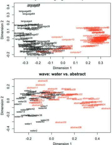
7. Pairwise similarities between all concordance-based vectors are computed, using the cosine as a similarity measure. This step yields the result of a distance matrix that captures similarities and differences across all concordance lines. This data structure is the token-based semantic vector space that can now be investigated. 8. A method of analysis that suggests itself for further investigations is the visualization of the token-based semantic vector space as a cloud of data points on a two-dimensional graph (cf. Heylen et al. 2012). For our purposes, we used metric multidimensional scaling to transform the vectors of PMI values for each concordance line into values on two dimensions that can be projected onto such a graph. Figure 1 presents visualizations of two analyses in which tokens of lexical elements are distinguished on the basis of their contexts. The analyses follow the steps that have been described above.
The first panel of Figure 1 shows that the token-based semantic vector space achieves a very good automatic discrimination between the nouns wish and fish. The graph presents a two-dimensional MDS solution of a semantic vector space that includes 133 vectors that are based on concordance lines of wish and 133 vectors that are based on concordance lines of fish. A logistic regression analysis that includes the first two dimensions of the MDS solution as predictor variables, both of which are significant predictors, achieves a classification accuracy of 89.8%. A high classification accuracy is of course to be expected, given that wish and fish are two different words with completely different meanings. It is instructive to look at some actual examples to see how the respective concordance lines are distributed in the cloud of data points. To the very left of the graph, the concordance lines fish88 and fish79 appear in close proximity. The context items in these concordance lines are shown below. It is evident that both concordance lines contain context items that are strong cues for the key word fish.
(9) fish79 <w vvd>cooked, <w nn2>sausages, <w nn2>chips, <w vvb>bet (10) fish88 <w nn1>lunch, <w itj>hello, <w nn2>beans, <w nn2>chips,
<w nn2>beans
The graph also shows a number of concordance lines for fish that are positioned far toward the right, so that they are actually misclassified by the logistic regression. Concordance lines of two such examples are shown below. None of the context items would evoke the connotation of fish in a human observer, and so it is understandable that the token-based semantic vector space does not associate these concordance lines with the key word fish.
(11) fish102 <w np0>india, <w nn2>trees, <w np0>india, <w nn1>farm (12) fish130 <w vvg>trading, <w np0>independent, <w av0>directly,
<w nn2>ports
Having established the general viability of using token-based semantic vector spaces for semantic analyses, we can move on to a more interesting test case for the method, namely the comparison of near-synonyms such as happy and glad. Since the adjectives happy and glad have partially overlapping meanings, they can occur in very similar contexts. The second panel of Figure 1 shows a two-dimensional MDS solution of a vector space based on 102 uses of happy and 102 uses of glad. It is apparent that these two are much harder to distinguish than wish and fish. A logistic regression analysis that includes the first two
dimensions of the MDS solution as significant predictor variables achieves only a classification accuracy of 64.2%. The right half of the graph shows a large area in which happy and glad overlap. To the left, however, there is a cloud of examples that is exclusively comprised of concordance lines of happy. This indicates that there are certain uses of happy in which the adjective cannot be replaced with glad. A manual inspection of these examples, three of which are given below, reveals that they typically involve the context item birthday and further context items that relate to either the song Happy Birthday or birthday congratulations in general.
(13) happy16 listen he’s playing happy birthday. Happy birthday happy17 happy birthday dear granddad, happy birthday to you
happy11 Back! Back! Sing happy birthday to you.
The contrast of happy and glad reveals that the method can not only pick up semantic differences but also sense relations such as (partial) synonymy. That is, if one of two synonymous items has a specific sub-sense that is not shared by the other item, this will be registered in the collocational behavior of the two, and it will become apparent when their collocational behavior is examined and visualized.
3.2 Distinguishing different word senses on the basis of their
contexts
Heylen et al. (2012) use token-based semantic vector spaces for the task of visualizing differences between different senses of polysemous items. We repli-cate their general approach in this section with comparisons of two English polysemous words, namely the nouns syntax and wave. The noun syntax does not only refer to the way in which languages combine words into phrases and sentences but also has a sense that relates to computer programming, specifi-cally to the “grammar” of programming languages. The two senses can be clearly distinguished on the basis of their collocational behavior: the expression syntax error is highly predictive of the computational sense, whereas ditransitive syntax is an expression that unambiguously points to the linguistic sense. The noun wave actually has a number of senses, many of which are figurative. In our analysis, we distinguish a sense that denotes the movement of water from all remaining senses, which we group together under the heading of abstract mean-ing. The latter comprises heat waves, waves of enthusiasm, and electromagnetic waves, to name but a few.
The actual analyses have been conducted in accordance with the technical steps that were discussed in the previous section, with the exception that in step one, only a single concordance was retrieved from the BNC, which was subse-quently annotated manually for the senses that we distinguish. As in the word comparisons that were discussed above, we contrast equal numbers of concor-dance lines per word sense, and each concorconcor-dance line is represented as a vector of PMI values that was put together on the basis of the context elements contained in that concordance line.
Figure 2 visualizes the two contrasts. The first panel, which is based on 134 concordance lines with 67 examples for each of the two word senses of syntax, shows a very clear discrimination of the two senses. This is due to the fact that in particular the computational sense is associated with a narrow range of words that are highly predictive cues. A logistic regression analysis establishes that only the
first dimension of the MDS solution in Figure 2 is a significant predictor variable, yet the classification accuracy is very high (94.8%). In the small area of overlap in the graph, we find examples in which linguistic examples involve context items such as processor, interface, or errors, which misleadingly point to the computa-tional sense. The second panel of Figure 2 shows the discrimination of the senses of wave. The analysis is based on 88 concordance lines. Also here, only the first dimension of the MDS solution is a significant predictor in a logistic regression analysis, but the model still achieves a classification accuracy of 80.7%.
In summary, our results corroborate the findings by Heylen et al. (2012), indicating that token-based semantic vector spaces are a useful tool for the distinction of concordance lines that represent different senses of the same word. There are many potential applications of this approach, not only in lexico-graphy, as suggested by Heylen et al. (2012), but also in research on polysemy (Glynn and Robinson 2014).
3.3 Distinguishing concordance lines from different texts
As a third practical application of our approach, we use token-based semantic vector spaces as an instrument to match concordance lines with the text from which they originate. Importantly, the concordance lines that we will deal with in this section do not share a common key word, but they are mere samples that are drawn from a larger text. Two corpus files from the BNC were randomly selected for this purpose. File ACB contains text from a children’s book and thus represents the text type of fictional prose; file A4H is taken from a periodical on world affairs. Example concordance lines from the respective texts are shown below.
(14) ACB-3 <w PNP>She <w VVD>kicked <w AV0>aside <w DT0>some <w PRF>of <w AT0>the <w NN1>mess <c PUN>, <w VVD-VVN>bent <w AVP>down <w TO0>to <w VVI>pick <w AVP>up <w AT0>a <w AJ0>crisp <w NN1>packet
ACB-50 <w AV0>headlong<c PUN>, <w PRP>over <w AT0>the <w NN1>town <c PUN>, <w TO0>to <w VVI>swim <w AV0>frantically <c PUN>, <w AV0>comically<c PUN>, <w PRP>in <w AJ0>empty <w NN1>air
(15) A4H-24 <w AJ0>tentative <w NN1>promise <w PRP>from <w AJ0>Hindu <w NN2>militants <w CJT>that <w AT0>the <w NN1>mosque <w VM0>would <w XX0>not <w VBI>be <w VVN>harmed
A4H-42 <w AT0>the <w NN2>Police <w NN0>department<c PUN>, <w XX0>not <w PRP>on <w AT0>the <w NN1>mayor <c PUN>-<w DTQ>which <w NP0>Mr <w NP0>Chirac <w NN2-VVZ>complains
<w VBZ>is
For a human observer, it would be quite easy to distinguish a sentence from a children’s book from a sentence that expresses political commentary, even in cases that contain words which would be perfectly expectable in either of the two text types, such as town, police, or complain. In order to test how token-based semantic vector spaces perform on this task, we retrieved 1,000 strings of 20 words from the respective corpus files and submitted them to the same procedure of steps that was used in the two previous sections. Figure 3 presents our results. The first panel
shows a contrast of the two corpus files on the basis of concordance lines that contain at least four context items that are contained in the type-based semantic vector space. This contrast distinguishes between 106 concordance lines, i.e. 53 from each text. In a logistic regression analysis, the first two dimensions of the MDS solution are selected as significant predictor variables, and the model achieves a classification accuracy of 91.5%. The second panel of Figure 3 illustrates how our approach performs when we reduce the number of context items that have to be present in a given concordance line. Since the vocabulary of our type-based semantic vector space is limited, many elements that are present in the full concordance lines do not feed into their respective representations. In a way, our approach thus mirrors the behavior of a reader who has a limited vocabulary and can base any guess about the provenance of a given concordance line only on that limited vocabulary. The accuracy of these guesses can be expected to decrease when our reader is allowed to guess on the basis of only two words, rather than four, that she or he recognizes in a given concordance line. If the minimum number of available context items is reduced to two items, we can draw on a set of 674 concordance lines. The second panel of Figure 3 shows that the discrimination is visibly less accurate, but classification accuracy is still high at 85.9%. The values of both axes are significant predictors of the two texts in a logistic regression model. We thus conclude that the approach is quite robust and allows accurate discrimi-nation of textual provenance even when the analysis is based on relatively few context items.
To conclude this short survey of practical applications that can be pursued with token-based semantic vector spaces, we hope to have given the reader a clear idea of how the approach works and what can be done with it. What we have not discussed so far is how the technique lends itself to the analysis of research questions that are anchored in a theoretical linguistic framework and that aim to test a given empirical hypothesis. The next section turns to this issue.
4 Token-based semantic vector spaces and the
asymmetric priming hypothesis
The case study in this section addresses a question within the general context of grammaticalization theory. Grammaticalization is the natural tendency of lan-guages to develop grammatical constructions, such as auxiliaries, tense markers, or clause connectors, out of lexical elements such as nouns or verbs. Hopper and Traugott (2003: xv) define grammaticalization as “the change whereby lexical terms and constructions come in certain linguistic contexts to serve grammatical
functions, and, once grammaticalized, continue to develop new grammatical functions”. A key aspect of grammaticalization is that it is hypothesized to change linguistic units in one direction only, namely from a lexical status toward an increasingly grammatical status. With regard to semantics, this implies that grammaticalizing units undergo a unidirectional change from highly specific and concrete meanings to more schematic and abstract meanings. The unidirec-tionality of semantic change in grammaticalization is broadly accepted as a statistical tendency. Counterexamples are recognized, but also their rarity is acknowledged (Norde 2009). What is more controversial is how the tendency of unidirectional change is to be explained. Jäger and Rosenbach (2008) propose that the psychological mechanism of priming can account for unidirectionality. Their argument, in a nutshell, is that the concrete meanings of lexical elements primes the more abstract meanings of their grammaticalizing counterparts, whereas the reverse does not happen to the same extent. Priming effects in real-time conversation are thus hypothesized to drive long-term historical shifts in meaning. Ever so gradually, meanings of grammaticalizing forms come to be associated with ever more abstract meanings, because the direction of priming is always toward greater abstraction. Jäger and Rosenbach articulate the asym-metric priming hypothesis in the following way (Jäger and Rosenbach 2008: 105):
[T]he idea we are advocating in this paper is the following: Unidirectional change ulti-mately goes back to the fact that a form or a concept/meaning A primes the use of a form or concept/meaning B if it is sufficiently similar to it, but that B doesn’t prime A. Via repeated usage and implicit learning B will become entrenched over time. That is, what appears as diachronic trajectories of unidirectional change is ultimately decomposable into atomic steps of asymmetric priming in language use. It is in this way that the actions of individual speakers may come to have a long-term impact on the shape of a grammar, without speakers consciously conspiring to change language in a certain direction.
On the asymmetric priming hypothesis, the lexical verb form going should thus prime the grammatical be going to construction in synchronic language use, but not vice versa. The question of whether concrete meanings are more likely to prime abstract meanings than the other way around is open to empirical study, and token-based semantic vector spaces lend themselves to such an analysis. Before we discuss an actual case study, it will be useful to spell out the predic-tions of the asymmetric priming hypothesis with regard to an application of token-based semantic vector spaces. What would we expect to see in the data?
First of all, it would be predicted that when two instances of used occur in relatively close proximity, we should frequently observe sequences of lexical-to-habitual, whereas sequences of habitual-to-lexical should be absent from the data, or at least less frequent than the opposite.
A second prediction is that a semantic vector space can detect a difference in meaning between a lexical source and its grammaticalized variant. For example, if we analyze a concordance of the verb form used, there should be an observable contrast between lexical uses of the form (e.g. He used a tooth-pick) and the weakly grammaticalized habitual marker used to VERB (He used to work at MIT). This prediction is of course not specific to the asymmetric priming hypothesis, but it reflects the general assumption that semantic change in grammaticalization is directional.
The third prediction concerns within-category sequences, in which a lexical instance of used is followed by another lexical instance, or in which two grammatical instances follow one another. Here, the asymmetric priming hypothesis predicts that shifts in meaning between the first and the second instance should be directed toward the area in semantic space that contains grammatical instances. In other words, there should be a recognizable semantic drift, even in within-category sequences. Importantly, this prediction cannot be tested on the grounds of simple text frequencies. Some semantic analysis has to enter the picture, and token-based semantic vector spaces offer a practical way of measuring the relevant meaning differences. The application of distributional techniques is furthermore attractive from a theoretical perspective. When lexical forms grammaticalize, they typically undergo a gradual process of change that has both formal and functional aspects. To take the well-known example of be going to, lexical uses that encode movement have ever so gradually been super-seded by uses that first encoded both movement and intention, then intention and future time reference but not necessarily movement, and then uses that encoded future time reference but not necessarily intention or movement (Bybee et al. 1994; Hilpert 2008: 118). While we could theoretically draw a line some-where on that continuum and treat one side as lexical and the other as gram-matical, the idea of gradience in grammaticalization has come to be accepted as a broad consensus (cf. Traugott and Trousdale 2010; Traugott and Trousdale 2013). Given that we expect uses of be going to (or indeed any other grammati-calizing construction) to change gradually in meaning, there will always be a spectrum of variability in meaning at any particular point in time. That is, with a token-based semantic vector space we can distinguish individual uses that are leaning more toward the lexical end of the spectrum from other uses that are leaning more toward the grammatical end of the spectrum, without having to adopt an arbitrary cut-off point to classify these uses as either lexical or gram-matical. With regard to the asymmetric priming hypothesis, this kind of differ-entiation affords a much more fine-grained and hence much more sensitive measure of potential priming effects. We can not only test whether there are priming effects between any two subsequent uses that fall into either of the two
categories of lexical or grammatical, but we can also test whether there are tendencies of semantic drift between any two subsequent uses from the entire meaning spectrum.
Finally, a fourth prediction can be made about the relative magnitude of semantic shifts between a first and a second instance of used. Since grammatical used to VERB would be expected to function as an attractor, shifts in its direction can be expected to traverse long distances in semantic space, whereas shifts in the opposite direction would be expected to traverse relatively shorter distances on average. This prediction can be motivated as follows. On the asymmetric priming hypothesis, a lexical element used, i.e. the prime, triggers a cognitive association with habituality that may result in a subsequent speech event in which grammatical used to VERB, the target, is uttered. This is predicted to be the case regardless of the position of lexical used in the semantic space. As a consequence, some of the pairs of prime and target may be fairly distant in that space. The asymmetric priming hypothesis further predicts that grammatical primes should only prime their own category, that is, further speech events of used to VERB that are semantically relatively close to the prime. What this means is that pairs of prime and target that go from lexical to grammatical have a relatively greater likelihood to traverse a long semantic distance.
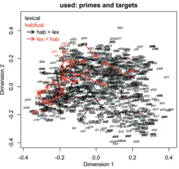
In order to test these predictions, we created a token-based semantic vector space on the basis of a concordance of the verb form used, which occurs about 66,000 times in the BNC. From this concordance, we selected pairs of instances that occurred within a distance of at least 20 but at most 50 words. These instances were submitted to the procedure that was discussed in Section 3. This procedure yielded 639 pairs of concordance lines. The approach here is completely analogous to the one that was taken in Section 3.2, where we tried to disambiguate different senses of the same words. As in the cases of syntax and wave that were described above, the concordance lines of used were manually categorized as instantiating either the lexical verb use or the grammaticalized construction used to VERB. Each concordance line was further coded as either being a prime (i.e. the first instance in a sequence) or a target (i.e. the second instance in a sequence). Figure 4 visualizes the semantic vector space. The graph is based on 1,278 concordance lines with 639 primes and 639 targets. All data points are labeled with a letter and a running number. A“p” stands for primes, a “t” stands for targets, and the running numbers allow for the identification of pairs. Data points in black represent concordance lines with lexical meaning, whereas data points in red represent concordance lines with grammatical, habitual meaning. The arrows in the graph represent pairs in which prime and target belong to different categories. A red arrow signifies the kind of switch that would be predicted by the asymmetric priming hypothesis: An instance of
lexical used is followed by an instance of grammaticalized used to VERB. Black arrows represent switches in the opposite direction, i.e. from grammatical to lexical. All data points in the graph that are not connected by arrows represent within-category sequences. It is apparent that this is the case for the majority of pairs. On the basis of the graph, we can now evaluate whether the example of used and used to VERB yields results that are in line with the asymmetric priming hypothesis.
The first prediction concerned cross-category sequences. Relatively more sequences of lexical-to-grammatical were expected. In Figure 4, these are visua-lized as red arrows. Table 7 shows that this prediction is not borne out. In the table, observed frequencies are followed by expected frequencies in brackets. A first thing that the table shows is that within-category sequences are observed more often than expected. This can be interpreted as a priming effect: If a language user has recently processed habitual used to VERB, that form has an
Figure 4: A token-based semantic vector space of a concordance of used.
Table 7: Cross-category and within-category sequences.
target: habitual target: lexical prime: habitual (.) (.) prime: lexical (.) (.)
increased likelihood of recurring in the right context. With regard to cross-category sequences, the asymmetric priming hypothesis predicts that there should be more sequences of lexical-to-habitual than vice versa. The table shows that both types of cross-category sequences are significantly underrepresented (X2= 159.47, df = 1, p<0.001). This detracts from the asymmetric priming
hypothesis.
The second prediction was that the semantic vector space would detect a semantic difference between used and used to VERB. Also this prediction is borne out, as the instances of used to VERB cluster at the left edge of the semantic vector space. A logistic regression analysis with the first two dimen-sions of the MDS solution as predictor variables retains both axes as significant predictors. This result is however in need of qualification, since it does not yield a satisfactory classification accuracy. As can be seen in Figure 4, the lexical tokens of used in the dataset vastly outnumber the habitual tokens of used. Since our dataset is balanced for the tokens of primes and targets, but retrieval was blind to meaning, it suffers from the problem of unbalanced classes (Izenman 2008: 547). Addressing this problem is beyond the scope of the current study, not only because it has received little attention in linguistic work up to this point but also because it does not affect our conclusions from the analysis.
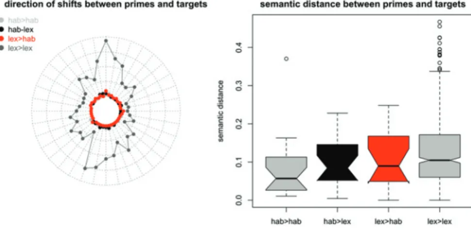
The third prediction posited a semantic drift for all sequences of primes and targets. On average, targets should be closer to the cluster of used to VERB at the left edge of the semantic vector space. The graph in Figure 4 does not reveal anything about the direction of within-category sequences, but it can be seen that the red and black arrows are criss-crossing the graph in a pattern that appears more or less random. The spider graph in the first panel of Figure 5 represents the
directions between primes and targets of all sequences in the dataset, thus allowing for a more systematic assessment. The orientation of the spider graph mirrors exactly dimensions 1 and 2 from Figure 4. Each data point shows how many shifts into a given direction are observed in our database. For example, the dark grey data point near the 12 o’clock position of the graph shows that upward-pointing shifts are relatively overrepresented in lexical-to-lexical sequences. The graph further reveals that none of the four types of sequence show a discernible drift toward the left side of the graph. This goes against the prediction of the asymmetric priming hypothesis.
The fourth and final prediction related to the magnitude of semantic changes in comparisons of primes and targets. Here, it was predicted that sequences of lexical-to-habitual would allow for the longest semantic leaps. The second panel of Figure 5 indicates that this prediction is not borne out either. The semantic distances between primes and targets in sequences of lexical-to-habitual are indistinguishable from the distances in habitual-to-lexical sequences.
In summary, the evidence from this case study does not support the asymmetric priming hypothesis. While the analysis reveals a strong effect of within-category priming, there is no asymmetry between sequences of lexical-to-habitual and habitual-to-lexical (cf. Table 7). The analysis in terms of a token-based semantic vector space complements and further supports this basic finding in important ways: There is also no observable semantic drift between primes and targets, even when they belong to the same category, and there is no difference in the magnitude of semantic leaps between lexical and grammatical targets.
It could of course be argued that the case of habitual used to is just one example, and that other contrasts might well reveal a different picture. In order to address this concern, we conducted three further analyses that repeat the analytical steps that were taken above with habitual used to with other examples. The forms that we have chosen for that purpose are the verb form got, the modal auxiliary may, and the connecting element since. What these forms have in common is that each of them has different uses that occupy different positions on a cline of grammaticalization. With got, we distinguish lexical uses from emerging modal uses. The modal auxiliary may, which is of course a fully grammaticalized element in all of its uses, exhibits traits of secondary grammaticalization in its uses with epistemic meaning. The same observation applies to since, which functions both as a preposition and as a conjunction. In its latter function, temporal meanings have given rise to the secondary grammaticalization of causal meanings. Table 8 offers illustrations of these contrasts.
For all three elements, we retrieved concordance lines from the BNC, selected pairs of occurrences that occurred within a window of at least 20 but at most 50 words, and annotated both primes and targets in terms of a binary seman-tic distinction that reflects degrees of grammaseman-ticalization, as illustrated in Table 8. Following the procedure that was discussed in Section 3, we created three semantic vector spaces for got, may, and since, which are represented in Figure 6.
With regard to our four predictions, the new analyses replicate the find-ings that we obtained earlier for habitual used to: Within-category priming is prevalent over cross-category priming in all three cases; no preference for lexical-to-grammatical sequences is detected. The semantic vector spaces allow us to discriminate with some success between the meanings that we captured in our semantic annotation. Logistic regression analyses with the first two dimensions of MDS solutions as predictor variables yield significant results. The disclaimers that were mentioned above with regard to the unba-lanced nature of the data apply here as well. As the arrows in the panels of Figure 6 show, there is no tendency of drift in the directions of prime-target sequences, nor is there a measurable difference in the magnitude of semantic shifts from prime to target when we compare lexical-to-grammatical sequences with grammatical-to-lexical sequences.2In sum, we submit that the results of
our earlier case study can be generalized to other pairs of lexical and gram-maticalized elements, and our results suggest that this observation even holds for grammaticalized elements with counterparts that have undergone second-ary grammaticalization.
Table 8: Different uses of got, may, and since.
lexical/less grammaticalized grammatical/more grammaticalized got We’ve got high-rise buildings in the city
of Nottingham.
He’s got to learn to stop sometimes. may Sporting equipment may be carried as
part of your baggage.
Training in the form of distance learning may become more important.
since Relations with Sri Lanka have improved markedly since the change of government last weekend.
The variable ‘costs’ starts from zero, since labour and material are not consumed until production starts.
2 The detailed results of these case studies are listed in Appendix A, and they are part of the supplementary materials that are available from the authors upon request.
5 Concluding remarks
This paper has presented token-based semantic vector spaces as a tool that can be applied in corpus-linguistic analyses such as word sense comparisons,
Figure 6: Token-based semantic vector space models of got, may and since.
comparisons of synonymous lexical items, and matching of concordance lines with a given text. We have demonstrated how corpus data needs to be processed in order to create semantic vector spaces, and we have offered a number of case studies that show the general viability of the approach and that illustrate the kinds of result that can be obtained with it. We further argued that token-based semantic vector spaces are not only useful for practical corpus-linguistic applications but also for the investigation of the-ory-driven questions. To illustrate this argument, we selected the asymmetric priming hypothesis (Jäger and Rosenbach 2008; Hilpert and Correia Saavedra 2016) as an example. The asymmetric priming hypothesis, which states that grammatical constructions will be primed by their lexical sources but not vice versa, has the virtue of making a number of empirically testable predictions. In Section 4 of this paper, we operationalized some of these predictions in such a way that they could be tested on the basis of a token-based semantic vector space. We conducted a case study of the lexical verb form used and its grammaticalized counterpart used to VERB, finding that the predictions of the asymmetric priming hypothesis could not be substantiated. These findings were replicated in three further case studies.
We end this paper by pointing to two possible applications of the approach that was presented here. The first of these concerns the notion of constructions in Construction Grammar (Goldberg 2006). In a recent paper, Lebani and Lenci (2016) show that type-based semantic vector spaces can successfully emulate speaker behavior in priming experiments. This result allows researchers in Construction Grammar to create explicit corpus-based models of speakers’ knowledge of constructions, which can then be tested against behavioral evidence. This triangulation of corpus data and experi-mental results can be developed further with semantic vector spaces that do not only account for types but also for tokens. A particular advantage of such an approach would be that it avoids a pitfall that type-based approaches have to struggle with, namely polysemy. A verb type such as get is highly polysemous, and it occurs in several syntactic environments. Its presence in the ditransitive construction (I got you some donuts) and in the intransitive motion construction (When do they get here?) might be taken to indicate that the two constructions are semantically related, when in fact the meaning of get across the two environments is markedly different. If the tokens around the verb are taken into account, this erroneous conclusion can be avoided.
The second application that we would like to mention is research into morphological and syntactic productivity. Again, we can point to an example in which type-based semantic vector spaces have been used to obtain useful
insights. Perek (2016) shows that the semantic distance between existing types of a productive process plays an important role. Areas in semantic space that are already filled by a cluster of existing types are likely to see even more types. In sparsely populated areas, new types are less likely to emerge. With token-based semantic vector spaces, these results can be further tested. In sum, we hope to have given the reader a primer of token-based semantic vector spaces that will hopefully encourage new and inter-esting research in the directions that we have suggested.
Funding: This work was supported by Schweizerischer Nationalfonds zur Förderung der Wissenschaftlichen Forschung (Grant/Award Number: ‘100015_149176/1’).
Appendix A: Results of the case studies on got,
may, and since
Table 11: Cross- and within-category sequences with since (X2= 77.803, df = 1, p = 2.745e-11).
target: causal target: temporal prime: causal (.) (.) prime: temporal (.) (.) Table 9: Cross- and within-category sequences with got (X2= 44.351, df = 1, p<0.001).
target: lexical target: modal prime: lexical (.) (.) prime: modal (.) (.)
Table 10: Cross- and within-category sequences with may (X2= 76.688, df = 1, p<0.001).
target: deontic target: epistemic prime: deontic (.) (.) prime: epistemic (.) (.)
References
Bybee, Joan L., Revere Perkins & William Pagliuca. 1994. The evolution of grammar: Tense, aspect and modality in the languages of the world. Chicago: University of Chicago Press. Davies, Mark. 2004. BYU-BNC. Based on the British National Corpus from Oxford University
Press. Available online at http://corpus.byu.edu/bnc/.
Firth, John R. 1957. A synopsis of linguistic theory 1930–1955. In Studies in linguistic analysis, 1–32. Oxford: Blackwell.
Glynn, Dylan & Justyna Robinson. 2014. Corpus methods in cognitive semantics. Studies in synonymy and polysemy. Amsterdam: John Benjamins.
Goldberg, Adele. E. 2006. Constructions at work: The nature of generalization in language. Oxford: Oxford University Press.
Heylen, Kris, Dirk Speelman & Dirk Geeraerts. 2012. Looking at word meaning. An interactive visualization of semantic vector spaces for dutch synsets. In Proceedings of the EACL-2012 joint workshop of LINGVIS & UNCLH: Visualization of Language Patters and Uncovering Language History from Multilingual Resources, 16–24.
Heylen, Kris, Thomas Wielfaert, Dirk Speelman & Dirk Geeraerts. 2015. Monitoring polysemy. Word space models as a tool for large-scale lexical semantic analysis. Lingua 157. 153–172. Hilpert, Martin. 2008. Germanic future constructions. A usage-based approach to language
change. Amsterdam: John Benjamins.
Hilpert, Martin & David Correia Saavedra. 2016. The unidirectionality of semantic changes in grammaticalization: An experimental approach to the asymmetric priming hypothesis. English Language and Linguistics. https://doi.org/10.1017/S1360674316000496. Hilpert, Martin & Florent Perek. 2015. Meaning change in a petri dish: Constructions, semantic
vector spaces, and motion charts. Linguistics Vanguard.
Izenman, Alan J. 2008. Modern multivariate statistical techniques. Regression, classification, and manifold learning. New York: Springer.
Jäger, Gerhard & Anette Rosenbach. 2008. Priming and unidirectional language change. Theoretical Linguistics 34(2). 85–113.
Jenset, Gard B. 2013. Mapping meaning with distributional methods. A diachronic corpus-based study of existential there. Journal of Historical Linguistics 3(2). 272–306.
Kiela, Douwe & Stephen Clark. 2014. A systematic study of semantic vector space model parameters. Proceedings of EACL 2014, Second Workshop on Continuous Vector Space Models and their Compositionality (CVSC), Gothenburg, Sweden, 21–30.
Lebani, Gianluca & Alessandro Lenci. 2016. “Beware the Jabberwock, dear reader!” Testing the distributional reality of construction semantics. Proceedings of the 5th Workshop on Cognitive Aspects of the Lexicon (CogALex-V), 8–18.
Table 12: Mean magnitudes of semantic leaps between prime and target.
lex>lex lex>gram gram>lex gram>gram got . (sd .) . (sd .) . (sd .) . (sd .) may . (sd .) . (sd .) . (sd .) . (sd .) since . (sd .) . (sd .) . (sd .) . (sd .)
Leech, Geoffrey. 1992. 100 million words of English: the British National Corpus. Language Research 28(1). 1–13.
Levshina, Natalia. 2015. How to do Linguistics with R: Data exploration and statistical analysis. Amsterdam: John Benjamins.
Norde, Muriel. 2009. Degrammaticalization. Oxford: Oxford University Press.
Perek, Florent. 2016. Using distributional semantics to study syntactic productivity in diachrony: A case study. Linguistics 54(1). 149–188.
Ruette, Tom, Dirk Speelman & Dirk Geeraerts. 2013. Lexical variation in aggregate perspective. In Augusto Soares Da Silva (ed.), Pluricentricity: Linguistic variation and sociocognitive dimensions, 95–116. Berlin: De Gruyter.
Sagi, Eyal, Stefan Kaufmann, and Brady Clark. 2011. Tracing semantic change with latent semantic analysis. In Justyna Robynson and Kathryn Allan (eds.), Current methods in historical semantics, 161–183. Berlin: De Gruyter.
Schütze, Hinrich. 1998. Automatic word sense discrimination. Computational Linguistics 24(1). 97–124.
Traugott, Elizabeth Closs & Graeme Trousdale (eds.) 2010. Gradience, gradualness and gram-maticalization. Amsterdam: John Benjamins.
Traugott, Elizabeth Closs & Graeme Trousdale. 2013. Constructionalization and constructional changes. Oxford: Oxford University Press.
Turney, Peter D. & Patrick Pantel. 2010. From frequency to meaning: Vector space models of semantics. Journal of Artificial Intelligence Research 37. 141–188.
Wheeler, Eric S. 2005. Multidimensional scaling for linguistics. In Reinhard Koehler, Gabriel Altmann & Raimond G. Piotrowski (eds.), Quantitative linguistics. An international handbook, 548–553. Berlin: De Gruyter.