Altimetric sampling and mapping procedures induce spatial and temporal aliasing of the signal – characteristics of these aliasing effects in the Mediterranean Sea

(1)

HAL Id: hal-00331132

https://hal.archives-ouvertes.fr/hal-00331132

Submitted on 17 Jul 2007

HAL is a multi-disciplinary open access

archive for the deposit and dissemination of sci-entific research documents, whether they are pub-lished or not. The documents may come from teaching and research institutions in France or abroad, or from public or private research centers.

L’archive ouverte pluridisciplinaire HAL, est destinée au dépôt et à la diffusion de documents scientifiques de niveau recherche, publiés ou non, émanant des établissements d’enseignement et de recherche français ou étrangers, des laboratoires publics ou privés.

Altimetric sampling and mapping procedures induce

spatial and temporal aliasing of the signal –

characteristics of these aliasing effects in the

Mediterranean Sea

M.-I. Pujol, G. Larnicol, G. Dibarboure, F. Briol

To cite this version:

M.-I. Pujol, G. Larnicol, G. Dibarboure, F. Briol. Altimetric sampling and mapping procedures induce spatial and temporal aliasing of the signal – characteristics of these aliasing effects in the Mediterranean Sea. Ocean Science Discussions, European Geosciences Union, 2007, 4 (4), pp.571-622. �hal-00331132�

(2)

OSD

4, 571–622, 2007

Altimetric data in the Mediterranean Sea

M.-I. Pujol et al.

Title Page Abstract Introduction Conclusions References Tables Figures ◭ ◮ ◭ ◮ Back Close

Full Screen / Esc

Printer-friendly Version

Interactive Discussion

EGU

Ocean Sci. Discuss., 4, 571–622, 2007 www.ocean-sci-discuss.net/4/571/2007/ © Author(s) 2007. This work is licensed under a Creative Commons License.

Ocean Science Discussions

Papers published in Ocean Science Discussions are under open-access review for the journal Ocean Science

Altimetric sampling and mapping

procedures induce spatial and temporal

aliasing of the signal – characteristics of

these aliasing effects in the

Mediterranean Sea

M.-I. Pujol1, G. Larnicol2, G. Dibarboure2, and F. Briol2 1

INGV, Via Donato Creti 12, 40128 Bologna, Italy 2

CLS Space Oceanography Division, 8–10 Rue Herm `es, 31526 Ramonville St. Agne, France Received: 15 May 2007 – Accepted: 18 June 2007 – Published: 17 July 2007

(3)

OSD

4, 571–622, 2007

M.-I. Pujol et al.

Full Screen / Esc

EGU

Abstract

This study deals with spatial and temporal aliasing of the sea surface signal and its restitution with altimetric maps of Sea Level Anomalies (SLA) in the Mediterranean Sea. Spatial and temporal altimetry sampling, combined with a mapping process, are unable to restore high-frequency (HF) surface variability. In the Mediterranean Sea,

5

it has been shown that signals whose intervals are less than 30–40 days are largely underestimated, and the residual HF restitution signal contains characteristic errors which make it possible to identify the spatial and temporal sampling of each satellite.

The origin of these errors is relatively complex. Three main effects are involved: the sampling of the HF long-wavelength (LW) signal, the correction of this signal’s aliasing

10

and the mapping procedure.

– The sampling depends on the characteristics of the satellites considered, but

gen-erally induces inter-track bias that needs to be corrected before the mapping pro-cedure is applied.

– Correcting the aliasing of the HF LW signal, carried out using a barotropic model

15

output and/or an empirical method, is not perfect. In fact, the baroclinic part of the HF LW signal is neglected and the numerical model’s capabilities are limited by the spatial resolution of the model and the forcing. The empirical method cannot precisely control the corrected signal.

– The mapping process, which is optimised to improve restitution of mesoscale

20

activity, does not propagate the LW signal far from the satellite tracks.

Even though these residual errors are very low with respect to the total signal, their signature may be visible on maps of SLAs. However, these errors can be corrected by more careful consideration of their characteristics in terms of spatial distribution induced by altimetric along-track sampling. They can also be attenuated by increasing

25

(4)

OSD

4, 571–622, 2007

M.-I. Pujol et al.

Full Screen / Esc

EGU

Ultimately, the HF signal, which is missing in maps of SLA, can be completed using a numerical model in order to estimate the total surface signal. The barotropic HF (<30 days) component accounts for nearly 10% of the total variability. Locally, it contributes nearly 25% of the total variance.

1 Introduction

5

Since the 1990s, numerous efforts have been made to improve altimetric processing and obtain accuracy of almost 2 cm, thus improving the precision of SLA maps. These efforts consisted in the correction of along-track measurements (Le Traon and Ogor, 1998; Carr `ere et al., 2005; etc.) as well as improvements to the mapping procedure and its ability to merge information from different satellites (Ducet et al., 2000; Ayoub

10

et al., 1998; Le Traon et al., 1995, 1998; etc.). In this way, global ocean products were largely improved. However, studies of limited areas have led us to continue the work already begun in order to improve restitution of SLA in these limited areas. In the case of the Mediterranean Sea, most of the improvements to altimetric processing have been achieved in the context of the MERSEA/MFSTEP projects. Studies using altimetry data

15

dedicated to the Mediterranean Sea have demonstrated the need to apply specific processing in this basin. In this paper, we focus on the difficulties involved in correcting the HF LW signal.

For the last few years, thanks to improvements in numerical models, it has been possible to estimate the HF LW surface variability with relatively high accuracy. Model

20

capabilities have been exploited to describe this signal and estimate its contribution to the total surface variability. The importance of this signal at high latitudes was under-lined by Fukumori et al. (1998) as the authors showed that at these latitudes, more than 50% of the signal variability in periods of less than 180 days can be accounted for by the signal for periods of less than 20 days. However, the Mediterranean Sea

25

was not included in the study area considered by the authors. So the HF LW surface variability in this basin has still not been well documented. Moreover, the HF variability

(5)

OSD

4, 571–622, 2007

M.-I. Pujol et al.

Full Screen / Esc

EGU

in the Mediterranean Sea also includes its specific response to inverse barometer (IB) variability. Le Traon and Gauzelin (1997) showed that the semi-enclosed character of the sea induces a delayed response to the IB in the basin.

Whereas the ability of altimetry data to observe a large part of the surface variabil-ity has essentially been demonstrated, the HF component still represents a significant

5

limit to the measurements. In fact, as the revisit frequency of the measurement is sev-eral days (10 days for TP and 35 days for ERS), the higher frequency signal is aliased. Moreover, the exploitation of altimetry data from gridded maps, which is often the case, implies that the HF LW variability is removed from the data before the mapping pro-cedure is applied in order to ensure the spatial coherence of the maps generated

10

(Le Traon et al., 1998). Correcting the HF signal from the altimetry data is also an important issue for altimetry data assimilation in numerical models. A first method-ology for correcting HF atmospheric effects was developed by Le Traon et al. (1998) and consisted in an empirical correction. More recently, another methodology, using a barotropic model output, which is a better way of taking into account the physical

15

process responsible for HF surface variability, was developed by Carr `ere et al. (2007)1. However, specific studies in the Mediterranean Sea have shown that these corrections, as currently used, do not entirely correct for the aliasing effect, leading to characteristic residual error signals on SLA maps.

This paper is organised as follows: in Sect. 2, the MOG2D and altimetry data set

20

used are described. In Sect. 3, the main characteristics of the HF (>30−1_days−1_{) LW}

barotropic signal given by the MOG2D model are described, and specific errors of the HF LW signal’s spatial and temporal aliasing are highlighted using an Observing System Simulation Experiment (OSSE). Section 4 focuses on the real altimetry data. The importance of the error signal was quantified from 11 years (1993–2003) of SLA

25

maps and solutions for correcting them have been included. In Sect. 5, the capabilities

1

Carr `ere, L., Volkov, D.,Le Traon, P.-Y., Schaeffer, P., Boone, C., Faug `ere, Y., and Gaspar, P.: Reducing the aliasing of the high frequency signals in altimeter data: empirical and model-based approaches, J. Atmos. Oceanic Technol., in review, 2007.

(6)

OSD

4, 571–622, 2007

M.-I. Pujol et al.

Full Screen / Esc

EGU

of the MOG2D numerical model are exploited to complete the altimetry data set and obtain an estimate of the total surface variability of the signal. Section 6 resumes and concludes this study.

2 Data processing

2.1 MOG2D model

5

In this study, the MOG2D model was used to obtain the high-frequency long-wavelength barotropic signal. MOG2D is a barotropic, non-linear, time step model which uses finite element spatial discretisation. The details of the model are given in Carr `ere and Lyard (2003).

The accuracy of this model in reproducing the HF barotropic variability was

demon-10

strated by Carr `ere (2003). However, its ability to reproduce the LF barotropic variability was limited by the considerable energy dissipation which was parameterised (Carr `ere, 2003).

The model was used in its global version without considering the gravity wave effect. It was forced with pressure and wind speed from the six-hour ECMWF analysis field

15

(ECMWF, 1991). The inverse barometer effect was removed from the output in order to consider only the dynamic part of the signal. The six-hour outputs of the model in the Mediterranean Sea over the 11-year period (1993–2003) were used. They were interpolated on 1/4◦_{regularly-gridded maps.}

2.2 Altimetry data

20

This study used altimetry data from the Topex/Poseidon (TP), Jason-1 (J1), Envisat (EN) and ERS-1/ERS-2 satellite altimeters over the 11-year period (1993–2003). The along-track data were combined and interpolated to build a homogeneous time set of weekly and regularly gridded (1/8◦

(7)

OSD

4, 571–622, 2007

M.-I. Pujol et al.

Full Screen / Esc

EGU

methodology used was the same as the one described by Larnicol et al. (2002), or Pujol and Larnicol (2005).

Complementary satellites were merged only twice: TP+ERS at the beginning of the period and J1+EN at the end.

Firstly, a homogeneous and inter-calibrated data set was obtained by performing a

5

global crossover adjustment, using T/P as the reference mission (Le Traon and Ogor, 1998). Then geophysical corrections (IB, tides, tropospheric, ionospheric) were ap-plied. Along-track data were resampled every 7 km using cubic splines and the SLA were computed by extracting a seven-year mean SSH corresponding to the (1993– 1999) period. Measurement noise was reduced by applying Lanczos (cut-off

wave-10

length of 42 km) and median (21 km) filters. An additional validation scheme was ap-plied to remove the remaining invalid points. This consisted in removing any data exhibiting differences which were too great when compared with the previous analysis (3 σ criteria).

Data were then interpolated over a regular 1/8◦

×1/8◦ grid, every seven days, using

15

an Objective Analysis (OA) method combining the different altimeter missions (Ducet et al., 2000) with a constant space and time isotropic correlation radius of 100 km and 10 days (Pujol and Larnicol, 2005). The presence of islands and complex coastlines was taken into account to avoid using observations that did not come from the same basin (i.e. Adriatic and Tyrrhenian Seas). Furthermore, measurement noise (variance

20

of 3 cm2 for T/P and J1, and 4.5 cm2 for ERS1/2 and EN) was corrected during the mapping procedure.

The LW signal was also taken into account. The performance of the different correc-tions has been analysed in this paper. In this way, three different altimetry data sets were generated. Two of them were generated using an empirical method described

25

by Le Traon et al. (1998). Its effect was to reduce inter-track bias mainly induced by the HF LW signal along-track sampling but also by errors in estimating the satellite’s orbit or correcting the inverse barometer effect that was not part of the dynamic sig-nal studied. This correction involves considering the bias as an along-track correlated

(8)

OSD

4, 571–622, 2007

M.-I. Pujol et al.

Full Screen / Esc

EGU

measurement error. This error enters into the estimate of the error covariance matri-ces needed in the OA mapping procedure. In practice, estimating this error covariance requires 1) an estimate of the variance associated with the inter-track bias and 2) a spatial/temporal domain in which data involved in covariance computation can be se-lected. Two different parameterisations were analysed. The first one considered the

5

error signal variance associated with the LW signal as 9 cm2for T/P and J1, and 15 cm2 for ERS1/2 and EN. For each measurement location, the correction was computed with respect to a spatial/temporal domain of 250 km and 10 days. The data set obtained with this correction was noted as AOS 250.

For the second experiment, the spatial/temporal domain was enlarged to 600 km and

10

10 days while the signal variance remained unchanged. This data set was noted as AOS 600.

The third data set was generated by applying a model-based LW correction as de-scribed by Carr `ere et al. (2007)1. The output of the MOG2D barotropic global ocean model, forced by the ECMWF surface pressure and wind speed, was considered to be

15

a good estimate of the HF LW surface variability to be corrected and was directly re-moved from the altimetry measurements. This model-based correction was completed with the previous empirical correction in order also to correct the signals which were not simulated with MOG2D, such as orbital errors or residual tidal correction. In this case, the variance associated with the signal was fixed at 9 cm2for T/P and J1, and 15 cm2

20

for ERS1/2 and EN. The correction was estimated considering a spatial/temporal range of 250 km and 10 days. The data set thus obtained was noted as AOS MOG2D. 2.3 Tide gauge data

Tide gauge data were compared with altimetry and model products. The mean part of the drifter data used was downloaded from the Italian agency APAT (Agenzia per la

25

Protezione dell’Ambiente et per I servizi Tecnici). Some of them come from the WOCE network (GLOSS/CLIVAR near real-time data).

(9)

OSD

4, 571–622, 2007

M.-I. Pujol et al.

Full Screen / Esc

EGU

order to be consistent with altimetry/MOG2D model data. Therefore, some specific corrections were applied. First ocean-tide signals were removed by applying different low-pass filters (Lef `evre and S ´enant, 2005). Then the static inverse barometer effect was removed from the data. Finally, original one-hour data were daily-averaged. Only daily means computed with a significant amount of data were considered. The limit

5

was arbitrarily fixed at 50% of the maximum amount of data possible. As some incon-sistencies in the time series available were observed (a bias may be detected after a manoeuvre involving the tide gauge station for instance), we considered each tide gauge station over different periods. The position and the different periods considered for each tide gauge station used are shown in Table 1.

10

3 Characterisation of the high-frequency aliasing effect in the Altimeter Observ-ing System

Mapped SLA products are often used to describe sea surface variability. However, these products do not allow us to restore the HF signal accurately. In fact, part of the signal is smoothed by the interpolation. Moreover, these SLA maps are usually

15

generated by merging the information from different altimeters, that sample the signal with different spatial coverage and revisit frequencies. Ultimately, both temporal and spatial aliasing of the HF signal are induced by the altimetric sampling and mapping procedure. The aim of this section is to characterise these aliasing effects.

3.1 Methodology

20

The aliasing effect induced by the Altimeter Observing System (AOS) was studied us-ing an OSSE.

Barotropic surface variability simulated with the MOG2D model (Sect. 2.1) was in-tended to represent the “true” surface signal.

First, a synthetic altimetric observation data set was obtained by interpolating this

(10)

OSD

4, 571–622, 2007

M.-I. Pujol et al.

Full Screen / Esc

EGU

“true” field on the altimetric measurement location. In this way, a spatial and linear interpolation was used.

Then, the along-track synthetic observations were used to restore the ocean sur-face state. Weekly gridded maps with 1/4◦ _{spatial resolution were generated. The}

methodology was the same as that described in Sect. 2.2 except that only LW errors

5

were considered. In particular, inter-satellite bias, measurement noise or orbit error, absent from the MOG2D output, were not reintroduced in the synthetic observation field. Synthetic altimetric observations were resampled every 7 km, then the OA was directly applied to generate weekly maps combining the different synthetic altimeter data sets, with a constant correlation range of 100 km and 10 days. Inter-track LW

10

errors, induced by the sampling of the HF LW surface signal, were corrected using the empirical method described by le Traon et al. (1998) (Sect. 2.2). Two parameter-isations were tested. The first one considered a spatial/temporal domain of 250 km and 10 days, and an error signal variance of 9 cm2and 15 cm2 for TP/J1 and ERS/EN respectively. In the following sections, the signal obtained with this parameterisation

15

will be noted as OSSE 250. The other parameterisation tested involved considering a spatial/temporal domain of 600 km and 10 days, while the variance of the error signal remained unchanged. This signal was noted as OSSE 600.

Finally, the reconstructed surface state thus obtained was compared to the “true” reference signal in order to identify the error signal induced by the HF aliasing in AOS.

20

This exercise was carried out over the 11-year period (1993–2003).

3.2 Principal characteristics of the barotropic dynamic signal in the Mediterranean Sea – description of the reference simulation

In this section, we describe the dynamic barotropic signal simulated by MOG2D and considered as the “true” reference signal. Here our intention is not to characterise this

25

signal fully, but rather to highlight its essential information, in order to introduce the study described in the subsequent sections.

(11)

OSD

4, 571–622, 2007

M.-I. Pujol et al.

Full Screen / Esc

EGU

variability with the AOS, we have mainly focused on the HF component of the signal. Here we considered the HF component as a signal whose frequency was higher than 30−1 _days−1

. This choice was determined by the difficulties in using altimetry data to restore this signal, as described in Sect. 3.4.

The mean variability (in term of variance) of the HF LW barotropic signal over the

5

[1993–2003] period is given in Fig. 1. The mean variance is nearly 7.6 cm2 over the whole sea. However, the mean variance is higher in the eastern part of the basin with 9 cm2compared with 7 cm2measured in the western part. Some specific areas of high HF barotropic variability (>15 cm2) have also been identified. This is the case in the northern Adriatic, the Gulf of Gab `es and the southern coast of the Ionian Sea or along

10

the Liguro-Provenc¸al coast especially in the Gulf of Lions. In these regions, the higher HF barotropic response is due to both the low bathymetry favourable to barotropic signals and the higher variable atmospheric forcing (surface pressure and winds) in these areas.

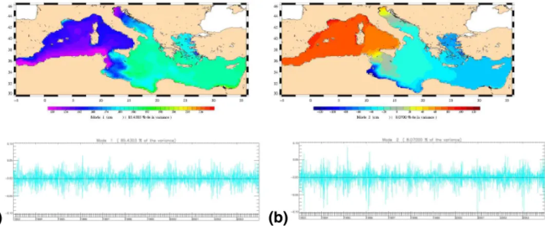
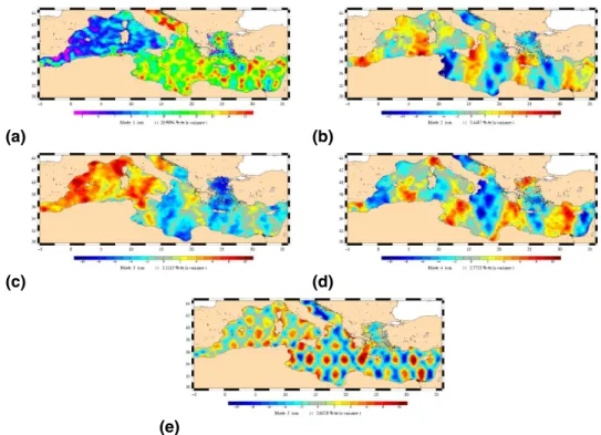
Finally the Empirical Orthogonal Function (EOF) decomposition for the HF LW

15

barotropic signal showed that the signal responsible for the variance observed can be summarised in two main modes shown in Fig. 2. The first mode, largely predominant, accounts for nearly 85.5% of the signal variance. It represents the mean variability of the basin, higher in the eastern part. The temporal component is clearly governed by a seasonal signal with higher variability in autumn/winter. The second mode, which

20

accounts for nearly 8% of the variance, suggests a western/eastern dipole variability induced by modulation in the Strait of Sicily. However, the variability observed in the Ionian Sea appears weaker than in the Levantine basin, except along the current in the southern Ionian. This mode’s temporal variability is also largely governed by a seasonal modulation of the signal, again with higher variability in autumn/winter.

25

While the low frequency (LF) barotropic component simulated by MOG2D is not re-alistic, since it is greatly attenuated by the energy-dissipation scheme (Carr `ere, 2003), its contribution to the variability of the total reference signal is not insignificant. In fact its contribution has the effect of increasing the signal’s mean variability by nearly

(12)

OSD

4, 571–622, 2007

M.-I. Pujol et al.

Full Screen / Esc

EGU

4.5 cm2bringing the signal’s total mean variability to 12 cm2. However, this contribution is nearly uniform over the whole sea and thus poorly modifies the main characteristics of the signal variability with respect to the HF component alone.

In this way, the EOF decomposition of the total simulated barotropic signal identified the same two main modes as previously described for the HF component alone. The

5

first main mode was responsible for 86.4% of the signal variance and the second mode accounted for 7.7% of the variance (not shown).

The results obtained with MOG2D indicate that wind speed and surface pressure are the main forcing factors responsible for barotropic HF LW surface variability (Carr `ere, 2003). However, the complexity of the phenomena involved makes it difficult to

deter-10

mine the direct relationship between the two signals. In fact, the response of the basin is also constrained by the presence of different straits. Fukumori et al. (2007) especially underlined the connection between intra-annual surface variability in the Mediterranean Sea and water mass exchange through the Strait of Gibraltar, showing that such basin-wide surface variability is induced by wind variability west of the Strait of Gibraltar.

15

Moreover, Le Traon and Gauzelin (1997) also showed that the relationship between atmospheric surface pressure and Mediterranean surface barotropic variability is mod-ulated by the Strait of Gibraltar. In fact the authors identified the delayed response of the basin to the inverse-barometer effect.

In the following sections we analyse the altimetric signal obtained using the OSSE in

20

order to explore how well the AOS rstores the surface signal, better characterising the aliasing effect of the measurement.

3.3 Ability of altimetry to restore the total signal

For this study, we considered the OSSE 250 (Sect. 3.1) signal over the period [1993– 2003]. In fact, the parameterisation used to generate this signal corresponds to the

25

one currently used for the Mediterranean Sea.

(13)

OSD

4, 571–622, 2007

M.-I. Pujol et al.

Full Screen / Esc

EGU

weaker than the reference signal (Sect. 3.2), can be directly associated with the ab-sence of the signal for intervals of less than 14 days (weekly maps, Sect. 3.1), whereas it represents a significant part of the variability in the reference MOG2D signal. How-ever the spatial distribution of the signal variability is well restored with the OSSE. The difference between the eastern and western basin is observed with nearly 2 cm2 of

5

variance in the western basin and nearly 3.5 cm2 in the eastern basin. Moreover, as highlighted with the reference MOG2D data set (Sect. 3.2), larger values are observed in specific areas like the Gulf of Lions (5 cm2), the northern Adriatic (7 cm2) the south-ern coast of the Ionian Sea (6 cm2), the Aegean Sea (6 cm2) and along the Levantine coasts (5 cm2).

10

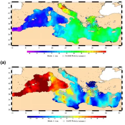
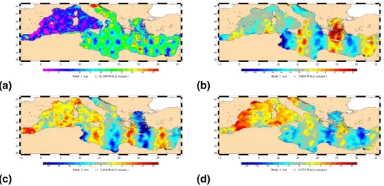
The EOF decomposition of this total OSSE 250 signal (Fig. 4) also revealed the main characteristics of the original signal. In fact, the first mode obtained clearly shows that the basin-wide variability is slightly greater in the eastern basin. This mode accounts for nearly 54% of the variance. As previously highlighted with the reference signal, this mode is also accompanied by a eastern/western basin balance, here identified with the

15

fourth mode, that accounts for nearly 3.6% of the variance. The annual modulation of the temporal components associated with these two modes (not shown) varies more in autumn/winter.

So ultimately, overall, the AOS correctly restores the signal’s main characteristics. However, its ability remains limited.

20

First for the frequencies actually restored: as mentioned earlier, the AOS is limited by the spatial revisit capability of the measurement that also limits the frequency of the maps generated. The weekly nature of the maps generated, limiting the reconstruction of the signal for intervals of higher than 14 days only, thus contributes to the weaker variance explained by both modes in the OSSE 250 signal with respect to the MOG2D

25

reference signal.

However, part of the real signal is aliased by the observing system, which also con-tributes to the alteration of the restored signal. In this way, as the reader has noted, the two characteristic modes deduced for the OSSE 250 signal (Fig. 4) are altered by

(14)

OSD

4, 571–622, 2007

M.-I. Pujol et al.

Full Screen / Esc

EGU

a shorter wavelength signal. This noise signal is characteristic of the aliasing effect in-duced by the altimetric sampling/mapping of the HF LW surface signal. It is discussed in Sect. 3.4.2.

Reducing this aliasing effect is a major challenge. First because it directly contributes to the better quality of the AOS products. In this way, the improved correction of the

5

aliasing effect also has a significant impact on many applications involving altimetry data. This is the case for instance with assimilation systems that need the utmost control of the altimetric signal.

However, even if it has been demonstrated to be efficient, the empirical correction used here does not allow us to control the signal ultimately extracted from the altimetric

10

measurement. Since fairly recently, better control of the corrected signal has been possible using a new kind of model-based correction. This suggests that the results presented before could be improved. However, as the principle of the OSSE was to consider such a model output as the reference signal, it is not possible for us to test this new kind of correction. The impact of such a MOG2D model-based correction will

15

be discussed in Sects. 4.2 and 5.2.

Finally, the correction of the HF LW signal in altimetry data raises some important questions. Which HF signal is observed by altimeters? Can we correct it without altering other signals? Which signal is ultimately restored by the AOS? When extracting the aliased HF signal from altimetry measurements, can we use it to estimate the total

20

surface signal, which is useful for many other studies? These are some of the many questions we have tried to answer in the following sections.

3.4 The altimetric observing system’s ability to restore the HF LW signal 3.4.1 Temporal aliasing effect

Normal and inevitable temporal aliasing of the HF signal is induced by the revisit

fre-25

quency of the measurements which is 10 days at best with TP and J1. While these two satellites allow us to observe signals accurately with intervals of greater than 20

(15)

OSD

4, 571–622, 2007

M.-I. Pujol et al.

Full Screen / Esc

EGU

days from along-track data, this limit is modified when the signal from gridded maps is considered. In fact, the gridded product results from the combination of different satel-lites with different revisit frequencies. Moreover, the mapped signal is altered by the smoothing effect inherent to the mapping procedure.

In order to determine the limit frequency restored from altimetric maps, we compared

5

the frequency spectrum of both the MOG2D reference signal and the signal restored using the OSSE 600 (Sect. 3.1). Choosing to use the OSSE 600 signal allowed us to limit the spatial aliasing effect as shown in the next section. However, the same study undertaken with OSSE 250 led to similar results (not shown).

Both the reference signal and the OSSE 600 signal frequency spectrum are given in

10

Fig. 5.

We first remind the reader that intervals of less than 14 days are not accessible from OSSE 600 (weekly maps, Sect. 3.1). The comparison of the two spectra clearly reveals that over 14 days, most of the signal is considerably under-estimated by the OSSE 600 signal. The exact limit of the frequency which is not under-estimated from

15

the OSSE 600 signal is difficult to identify. However, it can be considered that it is nearly 40−1_–30−1_days−1_{. The power of the reference MOG2D signal for the}

frequen-cies higher than 35 days−1_{is nearly 9.3 cm}2_{(2.36 cm}2_{between 35}−1_{and 14}−1_days−1_).

It falls to nearly 0.36 cm2for the OSSE 600 signal. Conversely, the lower frequency sig-nal is slightly overestimated in the OSSE 600 sigsig-nal. In fact, the power of this sigsig-nal

20

for frequencies lower than 35−1 _days−1 _{is 2.05 cm}2_{. It is 1.96 cm}2 _{for the reference}

MOG2D signal.

While the smoothing of the HF signal by the mapping procedure is inevitable, the importance of this smoothing as observed here must not be generalised to all existing altimetric mapped products. In fact, the HF signal reduction depends on the

differ-25

ent characteristics of the mapping procedure (number of satellites merged and their characteristics, frequency of the maps generated, correlation scales considered in the OA interpolation procedure, etc.). However, a study undertaken over the period [Oc-tober 2002–September 2005] where a four-satellite configuration was possible (with

(16)

OSD

4, 571–622, 2007

M.-I. Pujol et al.

Full Screen / Esc

EGU

ERS-2/EN, TP, J1 Geosat Follow On) showed that the difference between a two or four-satellite configuration was insignificant, since with four satellites the restored fre-quency limit was also nearly 40−1_–30−1_days−1_.

Finally, it can be considered that signals with intervals of less than 30 days are not accessible from the AOS mapped data as generated in Sect. 2.2. However, as an

5

accurate estimate of this signal is given by the MOG2D model, we can estimate its contribution to the total signal, as described in Sect. 5.

3.4.2 Spatial aliasing

Spatial noise induced by the signature of the HF LW signal on along-track data is identified when analysing the spatial structure of maps of the OSSE 250 signal. Here,

10

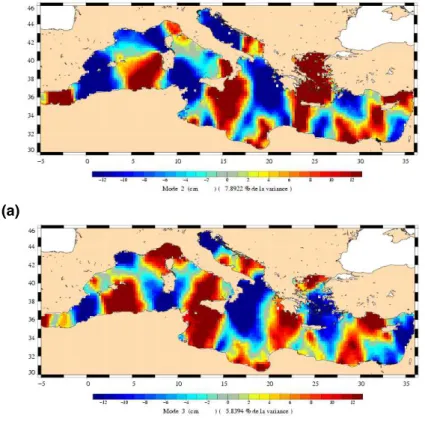
this signal was decomposed in EOF. The spatial component of the first four modes obtained is shown in Figs. 4 and 6.

As mentioned before (Sect. 3.3), two modes (the first and fourth) characterise the real surface signal. However they are altered due to the noise signal. The main part of this noise signal is clearly identified with the second and third modes. These two

15

modes account for respectively 7.9% and 5.8% of the variance. They clearly show a signal variability associated with the alternation of positive/negative vertically-oriented bands. The fact that this vertical-banded signal was not identified by the analysis of the MOG2D reference signal, leads us to suppose that it should not be interpreted as a real signal but rather as an error signal resulting from the altimetric along-track

20

sampling and mapping of the HF LW signal.

The spatial structure of the error signal revealed the characteristic sampling of the HF LW signal by the different altimeters, especially by ERS/EN. An example of this particular sampling will be given in Sect. 4.1, Fig. 9. The signature of the along-track bias in the generated maps can be explained by both the inefficiency of the LW signal

25

correction applied and the ineffectiveness of the mapping procedure in considering the along-track signal and propagating it in space in order to obtain spatially homogeneous maps. In fact, as the signal correlation scales used for the OA process have been

(17)

OSD

4, 571–622, 2007

M.-I. Pujol et al.

Full Screen / Esc

EGU

optimised for the restitution of the mesoscale signal (Pujol and Larnicol, 2005), they limit the OA’s ability to propagate the LW signal. The reduction of the error signal thus implies the direct reduction of the inter-track bias in order to limit residual errors due to the signal’s low spatial projection. Here the solution proposed was to consider more effectively the parameterisation of the empirical correction used (Le Traon et al., 1998)

5

(Sect. 2.2) in order to adjust it more closely to the characteristics of the signal in the Mediterranean Sea.

The spatial distribution of the error signal was taken into account in particular, leading to a re-estimate of the spatial domain of the data selection. In this way, instead of a range of 250 km, we applied a domain selection of 600 km that corresponded more or

10

less to the correlation scale of the spatial aliasing error signal described earlier. In fact, ∼600 km corresponds to the thickness of a coupled positive/negative band resulting from the sampling/mapping of the HF LW signal (visible on the second and third modes in Fig. 6). The OSSE signal thus generated was noted as OSSE 600 (Sect. 3.1).

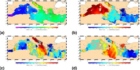
The results obtained are shown in Fig. 7. The EOF decomposition of the OSSE 600

15

signal revealed four main modes.

The first is explained by the mean basin-wide variability, slightly higher in the eastern basin. Here this mode accounts for nearly 71.1% of the signal variance which is much higher than the part of the variance accounted for by this mode in the OSSE 250 signal. Moreover, it should be noted that the spatial structure of this mode is clearer in the

20

OSSE 600 signal. As highlighted before, this mode must be coupled with the second mode that is explained by the eastern/western basin balance. Similarly to the first mode, accounting for 4.8% of the variance, this mode represents a greater part of the signal than observed for the OSSE 250 signal. This phenomenon is explained by the reduction of the error signal that also slightly alters this mode’s spatial structure.

25

Moreover, the spatial structure of the second mode corresponds better to its equivalent in the reference signal (Fig. 2), since the signal in the Ionian Sea is weaker. However, the next two modes seem to complete the variability in this basin. The third mode accounts for nearly 3.2% of the signal variance. It highlights the surface variability in

(18)

OSD

4, 571–622, 2007

M.-I. Pujol et al.

Full Screen / Esc

EGU

the Adriatic Sea and in the north-eastern part of the Ionian Sea. On the other hand, the fourth mode completes the variability in the rest of the Ionian Sea and is clearly in contrast to part of the activity in the Levantine Sea. This fourth mode accounts for 2.2% of the variance.

Finally, readjusting the empirical correction led to great results in terms of reducing

5

the errors of the aliased signal observed in the restored signal. However it did not lead to the total elimination of this signal since some residual error signals still alter the spatial structure of the modes observed. It clearly appears in the third mode, emphasising some satellite tracks (see for instance the Levantine basin). However, this residual error signal is now too weak to be explicitly accounted for by a dedicated

10

mode.

The results obtained with the empirical correction parameterised to a range of 600 km seem to indicate that this correction should be applied in the AOS in order to limit the error signal linked with the aliasing effect of the HF LW signal. However, this empirical correction does not allow us to control the signal which is ultimately extracted.

15

This problem should be resolved using a new kind of correction, which is better able to consider the physics of the surface due to the ability of the numerical models. This kind of correction, mentioned before, consists in directly extracting the HF LW signal from the along-track data, and identifying this signal from the numerical model. The success of such a correction, based on the MOG2D model, has already been demonstrated by

20

Carr `ere et al. (2007)1 for the global ocean, or by Manggiaroti and Lyard (2007) for the Mediterranean Sea. However, the latter authors only focused on interannual sig-nal restitution. The ability of this correction to improve the accuracy of the HF sigsig-nal (>30−1_days−1_{) restored with the AOS will be discussed in Sect. 4.2.}

4 Application to real data

25

Previously, the OSSE allowed us to identify specific problems linked to the HF LW surface signal aliasing effect induced by sampling/mapping the signal in the AOS. The

(19)

OSD

4, 571–622, 2007

M.-I. Pujol et al.

Full Screen / Esc

EGU

next sections are devoted to the analysis of the real signal restored with the SLA maps in the Mediterranean Sea. The importance of this noise signal and different solutions to minimise it were analysed.

4.1 Importance of the residual errors in the HF signal

As was previously identified with the OSSE 250 signal, we can observe in real SLA

5

maps some noise related to the sampling and mapping of the HF LW signal. This noise is highlighted by the EOF decomposition of the HF signal restored with maps of SLA. Here, the altimetric mapped data considered come from the AOS 250 data set, described in Sect. 2.2. Only the HF component of the SLA signal was considered. This signal was extracted applying a Loess time filter with a 30-day cut-off period.

10

This 30-day limit was chosen with reference to the results obtained in Sect. 3.4.1. It allows us to highlight the aliasing linked to the sampling/mapping of the HF LW signal since intervals of less than 30 days represent the part of the signal which is poorly restored. Moreover, this filtering limits the signal’s signature at lower frequencies, which is a strong component of the SLA signal (Larnicol et al., 2002; Pujol and Larnicol,

15

2005) and can completely mask the error signal we attempted to identify using EOF decomposition. The spatial component of the first five modes deduced from the EOF decomposition of the HF (>30−1_days−1_{) SLA signal are shown in Fig. 8.}

The first four modes have the same characteristics as the ones deduced from the OSSE 250 signal (Sect. 3.4.2, Figs. 4 and 6). The first and third modes represent the

20

signature of the HF LW signal: a basin-wide dominant variability more pronounced in the eastern basin, shown here with the first mode accounting for 21% of the signal vari-ance; and a balance between the western and eastern basin, here identified with the third mode that accounts for 3.1% of the variance. Both these modes have a tempo-ral component (not shown) that clearly shows a seasonal envelope for the signal with

25

stronger variability in autumn/winter. Of course, this signal’s amplitude as observed from weekly altimetric maps is essentially weaker than in reality (which, for these fre-quencies, is estimated with the MOG2D model (Sect. 3.2)) since we have seen that

(20)

OSD

4, 571–622, 2007

M.-I. Pujol et al.

Full Screen / Esc

EGU

the HF LW signal restored after along-track sampling and the mapping procedure is significantly underestimated for frequencies higher than 30−1_days−1 _{(Sect. 3.4.2).}

Moreover, the spatial structure of the first and third modes also show signals with small spatial scales, more pronounced in the eastern basin, and representative of a spatial aliasing effect resulting from the sampling/mapping procedures. For the third

5

mode, the noise has the same vertical-banded structure as previously highlighted with the OSSE 250 signal. Most of this noise is identified in both the second and fourth modes (Fig. 8). As observed before with the OSSE 250 signal, the variance explained by each of these two modes is as considerable as the third mode, with respectively 3.4% and 2.8% of the variance accounted for.

10

For the first mode, the noise signal that alters the spatial structure highlights the TP/J1 tracks. The main part of this noise is shown by the fifth mode that accounts for nearly 2.6% of the variance (Fig. 8). The reader will note that such a spatially-structured signal does not clearly appear in the OSSE 250 signal (Sect. 3). This seems to indi-cate that this error signal does not only involve HF LW barotropic sampling/mapping

15

difficulties. The source of this error signal is discussed in Sect. 4.3.

It is important to note that with respect to the total SLA signal, the variability linked to these error signals is very low. However, in some cases, their signature is directly visible on SLA maps. An example is shown in Figs. 9a and b. It represents the EN along-track data collected between 18 February and 3 March 2004 and the SLA map

20

generated for 25 February 2004 from these data (also combined with J1 data collected over the same period). The along-track data clearly show the specific “vertical-banded” structure resulting from the altimetric sampling of the HF LW signal. The SLA measured at the beginning of the period was strongly negative. It is visible along bold tracks, centred around 17◦_{E and 25}◦_{E. Conversely, at the end of the period SLA were} con-25

siderably positive as seen in fine tracks centred around 21◦_{E and 29}◦_{E. Whereas an}

empirical correction (Le Traon et al., 1998) was applied to the data to reduce this inter-track bias, and whereas the mapping process should also smooth this signal in order to obtain a homogeneous map, we can see on the gridded map obtained (Fig. 9b) that

(21)

OSD

4, 571–622, 2007

M.-I. Pujol et al.

Full Screen / Esc

EGU

the signature of these vertical bands still remain, highlighting the limits of the correction applied and of the mapping process.

The reader should note that this example is the strongest observed over a 12-year period. The limit of the correction for this example comes from both the large amplitude of the HF event over the eastern basin, and also from the lack of some EN tracks since

5

some data were rejected by the different selection/validation procedures applied to the data before mapping. This lack of data limits the impact of the empirical correction as it was parameterised.

Even if in the end, this error signal contributes little to the total variance of the total SLA signal, such a signature on SLA maps has enabled us to consider more carefully

10

the correction of the aliasing effect linked with the HF LW signal.

The OSSE study showed us that most of these errors can be removed using a better adjustment of the empirical correction used. However, as mentioned earlier, a new correction, which takes into account more carefully the physical characteristics of the HF surface signal, was also tested. This correction, based on the MOG2D model

15

output and described by Carr `ere et al. (2007)1was shown to improve the restitution of the interannual signal in the Mediterranean Sea (Mangiarotti and Lyard, 2007). Here we focus on the impact of the MOG2D model-based correction on the restitution of the HF signal.

4.2 Contribution of the MOG2D model-based correction

20

The MOG2D model’s contribution to reducing spatial aliasing errors in the Mediter-ranean Sea was evaluated by analysing the HF signal restored with the AOS MOG2D data set (Sect. 2.2). As done before, the HF (>30−1_days−1_{) component of the SLA}

was decomposed in EOF. The first four modes obtained (spatial component only) are shown in Fig. 10.

25

Two of these modes, the first and fourth, clearly show the characteristics of the real HF LW signal with a basin-wide variability more pronounced in the eastern part (first mode, accounting for 18.5% of the variance) and modulated with an eastern/western

(22)

OSD

4, 571–622, 2007

M.-I. Pujol et al.

Full Screen / Esc

EGU

basin balance (fourth mode, accounting for 2.5% of the variance).

However, theses two modes are strongly associated with the LW noise signal. In fact, it is clear that the first mode is also explained by the part of the noise signal highlighting the TP/J1 tracks. Contrary to the decomposition observed from maps of SLA corrected with the empirical method alone (Sect. 4.1), here this noise mode is

5

entirely restored by this first mode (it was previously characterised by the fifth mode; Fig. 8). Conversely, even though the fourth mode is also strongly affected by the LW error signal, the main part of this error signal is shown by both the second and third modes (explaining respectively 3.7% and 3.1% of the variance). They correspond to the vertical-banded error signal previously observed with the second and fourth modes

10

characteristic of the HF component of the SLA corrected with the empirical method alone (Sect. 4.1, Fig. 8).

The role of the MOG2D model-based correction in the global ocean has already been demonstrated by Carr `ere et al. (2007)1. The authors showed that this correction clearly contributed to reducing the variance of the error signal over the entire frequency

15

spectrum, thus leading to a better restitution of the total SLA signal than that obtained with the empirical correction alone. The contribution of the MOG2D model-based cor-rection over the Mediterranean Sea only has been studied by Mangiarotti and Lyard (2007). The authors focused on the interannual signal only and showed that it is better restored using this correction.

20

Conversely, the results obtained in this paper seem to indicate that the MOG2D model contributed not to reducing the error signal linked with sampling/mapping of the HF LW signal, but rather to reducing the role of the real HF LW signal reconstructed with maps of SLA. In fact whereas the residual HF LW signal explained nearly 24% of the variance when the empirical correction was considered (Sect. 4.1, Fig. 9), with the

25

MOG2D model-based correction, this signal accounted for only 21% of the variance, also considering the noise signal that highlighted the TP/J1 tracks. As a consequence, this led to a larger share of the variance being explained by the error signal.

(23)

OSD

4, 571–622, 2007

M.-I. Pujol et al.

Full Screen / Esc

EGU

First it is important to note that, contrary to the view of the authors cited earlier, the analysis focused on the HF signal (>30−1_days−1_{) that has been demonstrated as the}

hardest part of the signal to restore, and thus concentrates many kinds of error signal. The poor results obtained here with the MOG2D model also suggest that the er-ror signal observed does not involve the barotropic signal alone. In fact, while the

5

barotropic signal is the main component of HF surface variability at these latitudes (Fukumory et al., 1998), it does not represent all of the signal, especially when consid-ering lower frequencies than 20−1_days−1_{. As a consequence, this part of the signal is}

not included in the MOG2D output and therefore, aliasing errors induced by this signal cannot be reduced using the barotropic model’s contribution.

10

It is also important to note that the role of MOG2D was considered for frequencies higher than 20−1_days−1 _{only, with reference to the parameterisation adopted in the}

global ocean (Carr `ere et al., 20071). However, it was clearly shown that in the Mediter-ranean Sea, the signal with frequencies up to 40−1_–30−1_days−1 _{is aliased. This}

sug-gests that perhaps a better parameterisation of the MOG2D model-based correction

15

could improve the results obtained.

Moreover, as discussed before, the signature of the satellite tracks on maps of SLA also seems to reveal the difficulty the mapping procedure has in propagating the LW signal. This phenomenon must be linked with the parameterisation of the method, optimised for mesoscales rather than for LW signal reconstruction (Pujol and Larnicol,

20

2005).

Finally, as the MOG2D model-based correction needed to be completed with an empirical correction to be more efficient (Carr `ere et al., 20071), and as a re-parameterisation of the correction for the Mediterranean Sea alone involves a signifi-cant investment, even if the optimum results would be obtained with this model-based

25

correction, we chose to reduce the aliasing error signal identified using the empirical method alone. In fact, we previously demonstrated that an easy readjustment of the method would substantially improve the results obtained.

(24)

OSD

4, 571–622, 2007

M.-I. Pujol et al.

Full Screen / Esc

EGU

4.3 New parameterisation of the empirical correction

We saw in the OSSE study that improved consideration of the unique characteris-tics of the signal in the Mediterranean Sea for parameterising the empirical correction clearly improves this correction’s efficiency. Here, the new parameterisation tested consisted in enlarging the size of the spatial domain considered from 250 km to 600 km

5

(Sect. 3.4.2). This new parameterisation was applied in the AOS and the signal thus obtained was noted as AOS 600 (Sect. 2.2). The results obtained with this signal are described below.

An example of the results obtained with this new parameterisation is given in Fig. 9c. It corresponds to the map generated for 25 February 2004 from EN along-track data

10

collected between 18 February and 3 March and shown in Fig. 9a. The same map generated while applying the 250 km range parameter for the empirical correction is shown in Fig. 9b. It clearly demonstrates that the error signal we tried to reduce was largely reduced with the 600 km range parameterisation.

An EOF decomposition of the HF signal contained in maps generated while

apply-15

ing the 600 km range parameterisation (not shown) showed that these vertical-banded errors, highlighted by the second and fourth mode of variability when the 250 km range was used (Sect. 4.1, Fig. 8), are now absent, on account of the real signal (represented by first and third modes in Fig. 8) which is also less noisy than previously. Now the two representative modes account for respectively 22.7% (mode revealing the basin-wide

20

variation, greater in the eastern basin) and 3.3% of the variance (mode revealing the eastern/western balance).

However, the new parameterisation of the empirical correction does not correct all of the aliasing error signal. In fact, the mode highlighting the TP/J1 tracks (fifth mode in the signal decomposition corrected with the 250 km range parameter; Sect. 4.1,

25

Fig. 8) is still present in the signal corrected with the 600 km range parameter, where it represents the third mode of variability and accounts for nearly 2.5% of the variance. The persistence of this error signal reveals its complex origin, involving LW surface

(25)

OSD

4, 571–622, 2007

M.-I. Pujol et al.

Full Screen / Esc

EGU

variability (barotropic and non-barotropic components), its along-track sampling and its mapping. Here this signal seems to be explained by the signal’s higher variability in the TP/J1 inter-track due to the lack of more frequent data in these areas for estimating the signal. A similar EOF analysis of the HF signal was carried out over the period [2000–2005] when the SLA signal could be restored by merging the information from

5

three or four different altimeters (not shown). It revealed that this error signal strongly decreased since no significant signature was observed. This result tends to confirm that such an error signal results from the combination of satellite spatial coverage and the ability of the mapping procedure to extend the signal far beyond the track location. The reader will note that the improved correction of the signal was obtained simply by

10

changing the size of the selection domain. The variance associated with the inter-track bias error signal was unchanged. In fact, we consider that the values currently used (9 cm2for T/P and J1, and 15 cm2for ERS1/2 and EN) accurately represent this signal in the Mediterranean Sea. However, a sensitivity study was undertaken to evaluate the impact of these values on the inter-track bias correction. It showed the largely weaker

15

sensitivity of the results to this parameter rather than to the size of the domain defined. Moreover, it was shown that the HF LW signal was not entirely uniform over the basin (Sect. 3.2), suggesting that better results could be obtained when using a spatially variable variance associated with along-track bias, rather than spatially constant as is currently the case.

20

5 Merging MOG2D and altimetry data to obtain an estimate of the total surface variability

The results obtained before clearly showed that the SLA maps were unable to restore the total surface signal. In fact it was demonstrated that signals with frequencies higher than 40−1_–30−1_days−1 _{were strongly attenuated in the reconstructed altimetric signal} 25

(Sect. 3.4.1). On the other hand, barotropic variability, the main component of HF surface variability at these latitudes (Fukumori et al., 1998), was relatively well

(26)

repro-OSD

4, 571–622, 2007

M.-I. Pujol et al.

Full Screen / Esc

EGU

duced by numerical models. As the MOG2D model capabilities were demonstrated (Lyard and Roblou, 2003; Carr `ere and Lyard, 2003), it was used in conjunction with altimetry data to estimate the total surface signal in the Mediterranean Sea.

5.1 Methodology

The method used consisted in combining both complementary signals: respectively

5

the LF component of surface variability restored with the AOS, and the HF component modelled by the MOG2D model. The weekly altimetric maps (Sect. 2.2) were inter-polated daily (linear interpolation) and then combined with the daily mean of the 6-h output of the MOG2D model (Sect. 2.1). Both LF altimetric signal and HF MOG2D signal were obtained by applying a Lanczos low-pass filter.

10

A first test consisted in analysing the impact of the different HF LW signal correc-tions discussed earlier. Three different combinacorrec-tions were therefore compared. They consisted in combining the total MOG2D signal successively with the LF component of the AOS 250, AOS 600 and AOS MOG2D signals. The LF component was consid-ered as frequencies lower than 30−1_days−1 _{with reference to the results presented in} 15

Sect. 3.4.1. The three data sets thus obtained were noted as AOS 250 LF30+MOG2D, AOS 600 LF30+MOG2D and AOS MOG2D LF30+MOG2D. The comparison of the results obtained with these three different combinations is given in Sect. 5.2.1.

Subsequently, the sensitivity of the results to the filter cut-frequency applied to the different data sets to be combined was analysed. In this way, different combined data

20

sets were generated.

As a similar combination undertaken by Lyard and Roblou (2003) from the PSY2-v1 MERCATOR model showed that the LF component of the MOG2D signal significantly improved the results obtained, we first tested this signal’s contribution. Two different combinations were used. They combined the LF component of the AOS MOG2D

sig-25

nal with respectively the total MOG2D signal and the HF component of the MOG2D signal. Here the LF AOS MOG2D signal and the HF MOG2D signal were filtered with a 30−1_days−1 _{cut-frequency with reference to the results described in Sect. 3.4.1.}

(27)

OSD

4, 571–622, 2007

M.-I. Pujol et al.

Full Screen / Esc

EGU

The combinations thus obtained were noted as AOS MOG2D LF30+MOG2D and AOS MOG2D LF30+MOG2D HF30. The comparison of these two combinations is given in Sect. 5.2.2.

Finally, a third experiment was undertaken in order to test the sensitivity of the results to the cut-frequency used to extract the altimetric LF component. In

5

this way five combinations were compared. They consisted in combining the to-tal MOG2D signal with the LF component of the AOS MOG2D signal. Five cut-frequencies were applied: 20−1_{, 30}−1_{, 40}−1_{, 60}−1 _{and 80}−1_days−1_. _The

dif-ferent combinations thus obtained were noted as AOS MOG2D LF20+MOG2D, AOS MOG2D LF30+MOG2D, AOS MOG2D LF40+MOG2D, AOS MOG2D LF60+

10

MOG2D and AOS MOG2D LF80+MOG2D. The results obtained with these five com-bined signals are given in Sect. 5.2.3.

The accuracy of the different combinations generated was estimated by comparing them to different daily mean tide gauge data obtained over the 12-year period [1993– 2004] and given in Sect. 2.3.

15

5.2 Combined signal and tide gauge comparison 5.2.1 Sensitivity to the HF LW signal correction applied

As the sensitivity of the different HF LW signal corrections was discussed previously (Sect. 4) for the restored HF signal component, here three different combinations were compared to the tide gauge data, only considering the LF signal. In this way both tide

20

gauge data and the combined signal were filtered with a 20-day low-pass filter. The results obtained from comparing the LF component of the AOS 250 LF30+MOG2D, the AOS 600 LF30+MOG2D and the AOS MOG2D LF30+MOG2D signals with tide gauge data are given in Table 2.

As expected, they showed that the poorest results were obtained when the altimetric

25

signal was corrected by applying the empirical correction with a 250 km range param-eter. The mean correlation between tide gauge data and AOS 250 LF30+MOG2D

(28)

OSD

4, 571–622, 2007

M.-I. Pujol et al.

Full Screen / Esc

EGU

combined data was nearly 0.89. The variability of the difference between the two data sets represents nearly 27% of the tide gauge signal variability.

The best results were obtained with both the MOG2D model-based and the empirical correction with a 600 km range parameter. In fact, the mean correlation with the tide gauge data was nearly 0.9 for the two data sets and the error of the signal represented

5

nearly 25 to 26% of the signal variability.

However, the differences between the mean results remained very low. They were greater when considering each station independently. In fact, locally the impact of the MOG2D model-based correction led to an increase in the correlation with the tide gauge signal of 0.1 and a reduction in error representing more than 10% of the signal

10

variability. This was true for instance with the Imperia, Livorno and Ortona 1 stations where the MOG2D model-based correction clearly improved the signal restitution with respect to the empirical correction with the 250 km range parameterisation.

Conversely, few stations revealed that the empirical correction with a range of 250 km led to the best results. This was true for the Ancona, Crotone 2, Palinuro 4,

Portotor-15

res and Salerno 2 stations. However, the improvement remained lower than the one observed locally with the MOG2D model-based correction. In fact, the empirical correc-tion (250 km range) increased the correlacorrec-tion with the tide gauge signal by only 0.01 to 0.03 for the majority of the stations concerned. The improvement was significant only for the Salerno 2 station where an increase of nearly 0.08 of the correlation was

20

observed between the two combined signals. However, with nearly 0.69 of correlation for the best combination, it was also at this station that the poorest correspondence between combined and tide gauge signals was observed, which can be explained by the difficulty the AOS and the MOG2D signal have in accurately restoring the signal at the station location.

25

Some stations revealed that the empirical correction with the 600 km range param-eterisation led to the best results. However, the difference with the MOG2D model-based correction was generally low. They were significant for only two stations. At the Ortona 2 station, the empirical correction (600 km range) increased the correlation

(29)

OSD

4, 571–622, 2007

M.-I. Pujol et al.

Full Screen / Esc

EGU

with the tide gauge signal of 0.6 with respect to the MOG2D model-based correction. Likewise, the improvement of the correlation was nearly 0.9 at the Otranto 2 station.

The great variability of the results obtained can be explained by the complexity of the correction of the HF LW signal in the Mediterranean Sea. As the empirical correction needs to consider the signal in a spatial bubble, it limits the consideration of local

5

phenomenon, especially with the 600 km range parameterisation. Moreover, the quality of this correction is closely connected to the quality of the measurement, particularly sensitive in coastal areas. Conversely, the MOG2D model-based correction should make better allowance for local coastal phenomenon. However, this facility remains limited by the spatial resolution of the atmospheric forcing used and of the model grid.

10

The results obtained here are consistent with the ones given by Carr `ere et al. (2007)1 or Mangiarotti and Lyard (2007) that demonstrated the impact of the MOG2D model-based correction on the LF signal. However, the sensitivity to the results remains very low for a large number of the stations considered.

Finally, as the AOS MOG2D or AOS 600 signals led to similar results, it was decided

15

to pursue the study with the MOG2D model-based corrected signal. In fact, as men-tioned earlier, this correction allows better control of the corrected signal. Moreover, many of the residual errors previously identified (Sect. 4.2) in the HF component of the AOS signal when applying this correction have been removed here by the low-pass filtering of the AOS signal.

20

5.2.2 Impact of the HF MOG2D signal component

As Lyard and Roblou (2003) previously showed that the LF MOG2D signal could con-tain a complementary signal with respect to the PSY2v1 MERCATOR model, the complementarities of this signal with respect to AOS were tested. The two com-bined signals AOS MOG2D LF30+MOG2D and AOS MOG2D LF30+MOG2D HF30

25

were therefore compared. The results are given in Table 3.

They clearly showed that taking into account the LF component of the MOG2D sig-nal significantly improved the results obtained. In fact the mean correlation between