HAL Id: inria-00425383
https://hal.inria.fr/inria-00425383
Submitted on 12 Nov 2009
HAL is a multi-disciplinary open access
archive for the deposit and dissemination of
sci-entific research documents, whether they are
pub-lished or not. The documents may come from
teaching and research institutions in France or
abroad, or from public or private research centers.
L’archive ouverte pluridisciplinaire HAL, est
destinée au dépôt et à la diffusion de documents
scientifiques de niveau recherche, publiés ou non,
émanant des établissements d’enseignement et de
recherche français ou étrangers, des laboratoires
publics ou privés.
On the topology of planar algebraic curves
Jinsan Cheng, Sylvain Lazard, Luis Peñaranda, Marc Pouget, Fabrice
Rouillier, Elias P. Tsigaridas
To cite this version:
Jinsan Cheng, Sylvain Lazard, Luis Peñaranda, Marc Pouget, Fabrice Rouillier, et al.. On the topology
of planar algebraic curves. 25th annual symposium on Computational geometry - SCG 2009, Jun 2009,
Aarhus, Denmark. pp.361–370, �10.1145/1542362.1542424�. �inria-00425383�
On the Topology of Planar Algebraic Curves
Jinsan Cheng
∗Marc Pouget
∗Sylvain Lazard
∗Fabrice Rouillier
† INRIA France[email protected]
Luis Peñaranda
∗Elias Tsigaridas
‡ABSTRACT
We revisit the problem of computing the topology and geom-etry of a real algebraic plane curve. The topology is of prime interest but geometric information, such as the position of singular and critical points, is also relevant. A challenge is to compute efficiently this information for the given coordinate system even if the curve is not in generic position.
Previous methods based on the cylindrical algebraic de-composition (CAD) use sub-resultant sequences and com-putations with polynomials with algebraic coefficients. A novelty of our approach is to replace these tools by Gr¨obner basis computations and isolation with rational univariate representations. This has the advantage of avoiding compu-tations with polynomials with algebraic coefficients, even in non-generic positions. Our algorithm isolates critical points in boxes and computes a decomposition of the plane by rect-angular boxes. This decomposition also induces a new ap-proach for computing an arrangement of polylines isotopic to the input curve. We also present an analysis of the complex-ity of our algorithm. An implementation of our algorithm demonstrates its efficiency, in particular on high-degree non-generic curves.
Categories and Subject Descriptors
G.4 [Mathematical Software]: Algorithm design and analysis; I.1.4 [Symbolic and Algebraic Manipulation]: Applications; I.1.2 [Symbolic and Algebraic Manipula-tion]: Algorithms; I.3.5 [Computer Graphics]: Compu-tational Geometry and Object Modeling
General Terms
Algorithms, Experimentation.
∗LORIA - INRIA Nancy Grand Est, France.
†LIP6 - INRIA Paris-Rocquencourt - University Pierre et
Marie Curie, France.
‡INRIA Sophia-Antipolis M´editerran´ee & Laboratoire I3S,
UMR6070 CNRS, UNS France.
.
Keywords
Effective Algebraic Geometry, Exact Geometric Computa-tion, Topology of Algebraic Curves.
1.
INTRODUCTION
We consider the problem of computing a geometric rep-resentation of a planar real algebraic curve, C, defined in a Cartesian coordinate system by a bivariate polynomial f with rational coefficients, i.e., C = {(x, y) ∈ R2 | f (x, y) =
0} with f ∈ Q[x, y]. More precisely, we address the prob-lem of computing a planar graph whose vertices are mapped to points in the plane (possibly at infinity) and such that drawing the arcs as line segments gives a drawing isotopic1
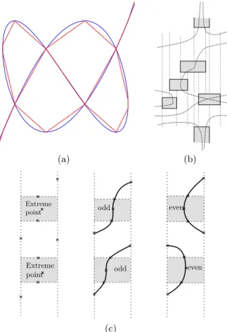
to the input curve (see Figure 1(a)).
In order to obtain an isotopic graph, the graph must con-tain vertices that correspond to self-intersections and iso-lated points of the curve. However, in order to avoid sep-arating such relevant points from other singularities (e.g., cusps), all singular points of C, that is, points at which the tangent is not well defined, are usually mapped to vertices of the graph. The graph must also contain vertices that cor-respond to points at infinity for each of the branches of C going to infinity. Finally, the graph should contain vertices corresponding to non-singular points on C so that drawing the arcs as line segments gives a drawing isotopic to C.
While singular points are needed for computing the topol-ogy of a curve, the extreme points of a curve are also very important for representing its geometry. Precisely, the ex-treme points of C for a particular direction, say the direc-tion of the x-axis, are the non-singular points of C at which the tangent line is vertical (i.e., parallel to the y-axis); the extreme points in the direction of the axis are called x-extreme. These extreme points are crucial for various ap-plications and, in particular, for computing arrangements of curves by a standard sweep-line approach [17]. Of course, one can theoretically compute an arrangement of algebraic curves by computing the topology of their product. How-ever, this approach is obviously highly inefficient compared to computing the topology of each input curve and, only then, computing the arrangement of all the curves with a sweep-line algorithm. Note that the x-extreme and singular points of C form together the x-critical points of the curve
1Even more precisely we want the curve C and the graph G
to be ambient isotopic in the real plane. In other words, we require the existence of a continuous map F : R2× [0, 1] −→
R2, such that Ftis an homeomorphism for any t ∈ [0, 1], F0
is the identity of R2 and F
(the x-coordinates of these points are exactly the positions of a vertical sweep line at which there may be a change in the number of intersection points with C).
It is thus useful to require that all the x-critical points of C are mapped to vertices of the graph we want to compute. To our knowledge, almost all methods for computing the topology of a curve compute the critical points of the curve and associate corresponding vertices in the graph. (Refer to [1, 9] for recent subdivision methods that avoid the compu-tation of non-singular critical points.) However, it should be stressed that almost all methods do not necessarily compute the critical points for the specified x-direction. Indeed, when the curve is not in generic position, that is, if two x-critical points have the same x-coordinate or if the curve admits a vertical asymptote, most algorithms shear the curve so that the resulting curve is in generic position. This is, however, an issue for several reasons. First, determining whether a curve is in generic position is not a trivial task and it is time consuming [23, 39]. Second, if one wants to compute ar-rangements of algebraic curves with a sweep-line approach, the extreme points of all the curves have to be computed for the same direction. Finally, if the coordinate system is sheared, the polynomial of the initial curve is transformed into a dense polynomial, which slows down, in practice, the computation of the critical points.
In this paper, given a curve C which is not necessar-ily in generic position, we aim at computing efficiently its topology, including all the critical points for the specified x-direction. In terms of efficiency, our primary goal is the practical efficiency (rather than worst-case complexity). In particular, we want to avoid computations with non-rational algebraic numbers or, equivalently in this context, algebraic computations such as Sturm sequences, Sturm-Habicht se-quences (which are a generalization of Sturm sese-quences, with better specialization properties [24]), and sub-resultant se-quences.
We review below previous work on the problem and then present our contributions.
Previous Work. There have been many papers address-ing the problem of computaddress-ing the topology of algebraic plane curves (or closely related problems) defined by a bivariate polynomial with rational coefficients [1, 2, 11, 4, 14, 20, 23, 25, 27, 33, 38, 6, 3, 32, 41, 13]. Most of the algorithms assume generic position for the input curve. As mentioned above, this is without loss of generality since we can always shear a curve into generic position [39, 23] but this has a sub-stantial negative impact on the time computation. All these algorithms perform the following phases. (1) Project the x-critical points of the curve on the x-axis, using sub-resultants sequences and isolate the real roots of the resulting univari-ate polynomial in x. This gives the x-coordinunivari-ates of all the x-critical points. (2) For each such value xi, compute the
intersection points between the curve C and the vertical line x = xi. (3) Through each of these points, determine the
number of branches of C coming from the left and going to the right. (4) Connect all these points appropriately.
The main difficulty in all these algorithms is to com-pute efficiently all the critical points in Phase 2 because the x-critical values in Phase 1 are, a priori, non-rational thus computing the corresponding y-coordinates in Phase 2 amounts, in general, to solving a univariate polynomial with non-rational coefficients and at least a multiple root (corre-sponding to the critical point). To this end, most algorithms
[2, 11, 4, 20, 23, 25, 27, 33, 38, 3, 41] rely heavily on com-putations with real algebraic numbers, Sturm sequences or sub-resultant sequences.
An approach using a variant of sub-resultant sequences for computing the critical points in Phase 2 was proposed by Hong [27]. He computed this way (xy-parallel) boxes with rational endpoints and separating the critical points. Count-ing the branches in Phase 3 can then be done by intersectCount-ing the boundary of the boxes with the curve which only involves univariate polynomials with rational coefficients. This ap-proach, see also [3, 32, 6] and the software package Cad2D2,
does not assume that the curve is in generic position. In a more recent paper, Gonz´alez-Vega and Necula [25] use Sturm-Habicht sequences which allow them to express the y-coordinate of the each critical point as a rational function of its x-coordinate. They implemented their algorithm in maple with symbolic methods modulo the fact that the al-gebraic coefficients of the polynomials in Phase 2 are approx-imated in fixed-precision arithmetic. The algorithm takes as a parameter the initial precision for the floating-point arith-metic and recursively increases the precision. This approach is however not certified in the case where the curve is not in generic position because the algorithm checks for the equal-ity of pairs of polynomials whose coefficients are evaluated (incorrect results have been reported in [40]). Note that there exists one variant of Gonz´alez-Vega and Necula algo-rithm that handles, without shearing, curves that are not in generic position [33]. This approach, however, requires sub-stantial additional time-consuming symbolic computations such as computing Sturm sequences.
Recently, Seidel and Wolpert [40] presented an alternate approach for computing the critical points avoiding most costly algebraic computations but to the expense of comput-ing several projections of the critical points. They project, in Phase 1, the x-critical points on both x and y-axes and also on a third random axis. After isolating the roots on each axis, they can recover (xy-parallel) boxes with ratio-nal endpoints that contain each exactly one critical point. From there, all computations only involve rational numbers but they, however, still need to compute Sturm-Habicht se-quences for refining the boxes containing the singular points until each box interests only the branches of the curve in-cident to the singular point. Their approach assumes that the curve is in generic position by a pre-processing phase in which the curve is sheared if needed. They also present a maple implementation, insulate, which is an implementa-tion of a certified algorithm for curves in arbitrary posiimplementa-tions. Note that their implementation does not report x-extreme points in the original system when the curved is sheared.
Even more recently, Eigenwillig et al. [14] (see also [28]) presented a variant of Gonz´alez-Vega and Necula approach, in which the roots of the polynomials with non-rational co-efficients are efficiently isolated using an implementation of a variant of an interval-based Descartes algorithm [15]. This variant, as [25], does not assume that the curve is in generic position but detects such configurations online. More pre-cisely, if the bit-stream Descartes algorithm is in, a sense, unlucky then, rather than refining down to a separation bound (e.g. [8, 31]), the algorithm shears the input curve and starts again. Note that this approach still computes Sturm-Habicht sequences for determining the polynomials
appearing in Phase 2 and the multiplicity of its multiple root. Also, if the curve is sheared to a (x′, y′) coordinate
sys-tem, they compute extreme points both for the x′-direction
and the direction corresponding to the x-axis. This approach has been implemented in C++ and is an implementation of a certified algorithm that handles curves that are not neces-sarily in generic positions and that reports x-extreme points for the original coordinate system.
Note finally that another approach that avoids expensive algebraic computations is to compute the critical or singular points using subdivision methods [1, 9]. The major draw-back of these methods is that, in order to certify the results, the subdivision has, in general, to reach a separation bound (certification can also be achieved by solving algebraic sys-tems by other means). It follows that, if no certification is required, these methods are very fast in practice, however, they can become very slow on difficult instances, if certifi-cation is required. To our knowledge, no implementation of such certified algorithm is available.
As for the complexity of the problem, the best known bound so far is eO(N12) [13], where N is essentially the
max-imum of the degree of f and of the maxmax-imum number of bits needed for representing the input coefficients and the notation eO denotes that the poly-logarithmic factors are omitted. This assumes that the real algebraic numbers are represented by isolating intervals. This complexity is based on theoretically fast computations with Sturm-Habicht se-quences and algorithms for univariate real root isolation.
Our contributions. We present an algorithm for comput-ing the topology of an algebraic plane curve which is possi-bly in non-generic position. The algorithm handles curves in non-generic positions in the Cartesian coordinate system in which they are defined. In particular, the algorithm never shears the coordinate system, which avoids the associated extra costs discussed above.
The other originality of our approach is that we succeed to avoid, in all cases, the computation of sub-resultant se-quences and computations with algebraic numbers; we use instead Gr¨obner bases and the rational univariate represen-tation. One can argue that these are just two different tool sets, this is true from a theoretical point of view but we show in the experiments the benefit of our choice when comput-ing with non-generic curves. Furthermore, the philosophy of our approach is to avoid, as much as possible, compu-tations that are time consuming in practice. This leads to various algorithmic choices such as avoiding the computa-tion of y-critical points and allowing the curve to intersect the top and bottom sides of boxes isolating x-extreme points (which avoids substantial subdivisions since the tangent at an extreme point is vertical).
The novelty of our algorithm mainly relies upon the use of three new ingredients for this problem. First, we use some of the state-of-the-art techniques to isolate the roots of bivari-ate systems, i.e., we use (i) Gr¨obner basis [19], (ii) Rational Univariate Representations (RUR) [35] which represent the roots of the system as rational functions of the roots of a uni-variate polynomial, and (iii) a subdivision technique based on Descartes’ rule of signs (and filtered with interval arith-metic for efficiency) for isolating the roots of the univariate polynomials [36, 16, 18]. Even though this approach is well known for system solving, it was not used before for com-puting the topology of algebraic curves.
Second, we compute and use the multiplicities in fibers (see Definition 1) of critical points to compute the topol-ogy at singular points and to do the connection at extreme points. For extreme points, we get these multiplicities by the RUR and a special case of a formula of Teissier [42]. For singular points, we solve the system of singular points with additional constraints. Note that the overall method to compute the topology at critical points is not new, it is described in full details in [40], see also for example [3, 27, 6, 32, 33, 1] for closely related approaches for curves in non-generic position. The novelty appears in the way we compute multiplicities in this context; once again we avoid computing sub-resultant sequences.
Third, we present a variant of the standard combinatorial part of the algorithm for computing the topology. We com-pute a decomposition of the plane (which is not a cylindrical algebraic decomposition) by rectangular boxes containing at most one critical point. Since we allow crossings on the top and bottom of extreme point boxes to avoid costly refine-ment of boxes, the connection is not always straightforward. To make the connection, we use the multiplicities in fibers of extreme points. Note that one advantage of this variant is that, even when the curve is in generic position, the al-gorithm does not require to refine these boxes until they do not overlap in x.
We also analyze the worst-case bit complexity of our algo-rithm. To the best of our knowledge, this is, for the problem considered here, the first time that the complexity of a (cer-tified) algorithm based on refinements and approximations is analyzed. Our technique, even though not novel, could presumably also be used to analyze the complexity of the algorithms in [25, 27, 40, 14].
Finally, we ran large scale benchmarks on over a thousand of curves during several weeks for comparing the different state-of-the-art available implementations.
The rest of the paper is organized as follows. First, we recall in Section 2 some basic material, in particular, on the multiplicity of the intersection of two curves and on Rational Univariate Representations of the roots of system of (alge-braic) equations. We present our algorithm in Section 3 and its complexity in Section 4. Finally, we present in Section 5 extensive experiments comparing various implementations.
2.
PRELIMINARIES
Let C, also denoted Cf, be a real algebraic plane curve
defined by a bivariate polynomial f in Q[x, y]. Since the geometry of the curve is not modified by taking the square-free part of f , we can assume without loss of generality that f is square-free. Note that C may consist of several alge-braic components, that is, f is not necessarily irreducible in R[x, y]. The algebraic components of the curve that are vertical lines (i.e., lines parallel to the y-axis) can be easily computed since their abscissa correspond to the real roots of the polynomial in x obtained as the gcd of the coefficients of f seen as a polynomial in y.
Partial derivatives are denoted with subscripts: for in-stance, fxdenotes the derivative of f with respect to x and
fyk (sometimes also fk) denotes the kthderivative with
re-spect to y. A point p = (α, β) ∈ C2 is called x-critical if
f (p) = fy(p) = 0, singular if f (p) = fx(p) = fy(p) = 0,
and x-extreme if f (p) = fy(p) = 0 and fx(p) 6= 0 (i.e., it is
x-critical and non-singular). Similarly are defined y-critical and y-extreme points. As x-critical and x-extreme points
are more often used in the following, we often simply refer to them as critical and extreme points.
The ideal generated by polynomials P1, . . . , Piis denoted
I(P1, . . . Pi). In the following, we often identify the ideal and
the system of equations {P1= 0, . . . , Pi= 0} (or any
equiv-alent system induced by a set of generators of the ideal). We consider, in particular, the ideals Ic = I(f, fy) and
Is = I(f, fx, fy); their roots are, respectively, the x-critical
and singular points of C.
Multiplicities.
We now recall the notion of multiplicity of the roots of an ideal, then we state two lemmata using this notion for study-ing the local topology at critical points. Geometrically, the notion of multiplicity of intersection of two regular curves is intuitive. If the intersection is transverse, the multiplic-ity is one; otherwise, it is greater than one and it measures the level of degeneracy of the tangential contact between the curves. Defining the multiplicity of the intersection of two curves at a point that is singular for one of them (or possibly both) is more involved and an abstract and general concept of multiplicity in an ideal is needed.
Definition 1 ([12, §4.2]). Let I be an ideal of Q[x, y] and denote Q the algebraic closure of Q. To each zero (α, β) of I corresponds a local ring (Q[x, y]/I)(α,β)obtained by
lo-calizing the ring Q[x, y]/I at the maximal ideal I(x−α, y−β). When this local ring is finite dimensional as Q-vector space, we say that (α, β) is an isolated zero of I and this dimension is called the multiplicity of (α, β) as a zero of I.
Let f, g ∈ Q[x, y] be such that the intersection of Cf and Cg
in C2 contains a zero-dimensional component equal to point
p = (α, β). Then (α, β) is an isolated zero of I(f, g) and its multiplicity, denoted by Int(f, g, p), is called the intersec-tion multiplicity of the two curves at this point.
We call a fiber a vertical line of equation x = α. For a point p = (α, β) on the curve Cf, we call the multiplicity of
β in the univariate polynomial f (α, y) the multiplicity of p in its fiber and denote it as mult(f (α, y), β).
The next lemma, due to Teissier [42], relates the multiplic-ity of a point in a fiber with the multiplicmultiplic-ity in the critical ideal. We will use it to deduce the multiplicity in the fiber knowing multiplicity in the ideal. More precisely, we will use the multiplicity in fibers of extreme points during the connection step of our algorithm.
Lemma 2 ([42][5, Lemma D.3.4]). For an x-extreme point p = (α, β) of f , mult(f (α, y), β) = Int(f, fy, p) + 1.
To compute the local topology of the curve at a singular point, we aim at isolating the singular point in a box so that the intersection of its border and the curve determines the topology. Indeed for a small enough box, the topology is given by the connection of the singular point with all the intersections on the border. So the box shall avoid parts of the curve not connected to the singular point. Knowing the multiplicity of the singular point in the fiber enables to isolate the singular point from other crossings of the curve in this fiber. Requiring in addition that intersections with the curve only occur on the left or right sides of the box leads to the following.3
3The proof is based on a recursive application of the mean
value theorem stating that the roots of the derivative of a polynomial P lie between those of P .
Lemma 3 ([40]). Let p = (α, β) be a real singular point of the curve Cf of multiplicity k in its fiber. Let B be a box
satisfying (i) B contains p and no other x-critical point, (ii) the function fyk does not vanish on B, and (iii) the curve
Cf crosses the border of B only on the left or the right sides.
Then the topology of the curve in B is given by connecting the singular point with all the intersections on the border. We now present the algebraic tools we use for isolating the roots of univariate and bivariate ideals.
Univariate Root Isolation.
We need to count and isolate the real roots of univari-ate polynomials, possibly in a given interval. This is, in particular, needed for computing the intersections between C and the sides of the boxes isolating the critical points. Only polynomials with rational coefficients will be consid-ered. The square-free part of the considered polynomials is first computed. The real roots are then isolated using recur-sive subdivision and the Descartes’ rule of signs (see [16, 18, 36] for details and [36] for the way interval arithmetic can be used to speed up computations). In our implementation, we use the RS software [37].
Rational Univariate Representation.
In our algorithm, we need to represent solutions of zero-dimensional ideals depending on two variables by boxes con-taining them. We use the so-called Rational Univariate Rep-resentation (RUR) of the roots, which can be viewed as a univariate equivalent to the studied ideal. The key feature of this RUR is the ability to isolate solutions in easily refinable boxes and to compute multiplicities.
Given a zero-dimensional ideal I = I(P1, . . . , Ps) where
the Pi ∈ Q[x1, . . . , xn], a Rational Univariate
Represen-tation of the solutions V(I) is given by F (t) = 0, x1 = G1(t)
G0(t), . . . , xn =
Gn(t)
G0(t), where F, G0, . . . , Gn are univariate
polynomials in Q[t] (where t is a new variable). All these uni-variate polynomials, and thus the RUR, are uniquely defined with respect to a given polynomial γ ∈ Q[x1, . . . , xn] which
is injective on V (I); γ is called the separating polynomial of the RUR. 4 Note that a random degree-one polynomial in
x1, . . . , xn is a separating polynomial with probability one.
The RUR defines a bijection between the (complex and real) roots of the ideal I and those of F . Furthermore, this bi-jection preserves the multiplicities and the real roots. Com-puting a box for a solution of the system is done by isolating the corresponding root of the univariate polynomial F and evaluating the coordinate functions with interval arithmetic. To refine a box, one just needs to refine the corresponding root of F and evaluate the coordinates again.
There exists several ways for computing a RUR. One can use the strategy from [35] which consists of computing a Gr¨obner basis of I and then to perform linear algebra op-erations to compute a separating element as well as the full expression of the RUR. The Gr¨obner basis computation can also be replaced by the generalized normal form from [34]. There exists more or less certified alternatives such as the Geometrical resolution [22] (it is probabilistic since the sep-arating element is randomly chosen and its validity is not checked, one also loses the multiplicities of the roots) or
re-4The polynomial F is the characteristic polynomial of
mγ, the multiplication operator by the polynomial γ, in
(a) (b) Extreme point Extreme point odd odd even even (c)
Figure 1: (a) Maple plot and isotopic graph computed by isotop of the curve of equation 16 x5
− 20 x3
+ 5 x − 4 y3
+ 3 y = 0. (b) Example of rectangle decomposition of the plane induced by the isolating boxes (critical and asymptotes). (c) Possi-ble connections involving extreme points.
sultant based strategies such as [29]. In our implementation, we use the strategy from [35] and compute Gr¨obner bases using the algorithm F5 [19].
3.
ALGORITHM
As discussed in Section 2, we consider, as input, a curve C without vertical components and defined by a square-free polynomial f ∈ Q[x, y] (note that our implementation does not require these assumptions, but the processing of vertical components is rather technical and we choose not to include all these details here). In a few words, the algorithm first focuses on critical points, their rational univariate represen-tations enable to compute multiplicities and boxes isolating each point with known topology inside the box. Then a sweep method computes a rectangular decomposition of the plane induced by the boxes of critical points. Eventually the connection is processed in all rectangles with a greedy method using multiplicities in fibers for extreme points. We describe more precisely our algorithm in six steps.
Step 1. Isolating boxes of the singular points and of the x-extreme points. As a general practical rule, the smaller the number of solutions of a system, the easier it is
to work with. Hence we split the system of critical points into the system of singular points and the system of extreme points. The system of singular points is the one of critical with in addition the equation fx= 0. The system of extreme
points, denoted Ie, is computed by saturation. Indeed, the
extreme points are critical for which fx 6= 0, thus we add
to the critical system the equation 1 − ufx = 0 with a new
variable u that we eliminate afterwards. We then compute the RURs of these systems Isand Ieand isolating boxes for
the solutions. We may need to refine the boxes of extreme and singular points to avoid overlaps.
Step 2. Multiplicities of critical points in fibers. For extreme points, we use the Teissier formula: the multiplicity of an extreme point in Ic is the same than in Ie because
precisely fxdoes not vanish at these points. The multiplicity
in Ie is given by the RUR, and hence the multiplicity of an
extreme point in its fiber is this number plus one according to the equation of Lemma 2.
For singular points, we use the definition of univariate multiplicity, namely the smallest integer k such that the kth
derivative no longer vanishes. Let Is,k be the system of
singular points with in addition the equations fyi = 0 for i
from 2 to k. Hence we solve, for k increasing from 2, the systems Is,kuntil it has no solutions. At each step, a singular
point which is no longer solution of Is,khas its multiplicity
in fiber equal to k.
Step 3. Refinement of the isolating boxes of the x-extreme points. Consider each such box, B, in turn. For each vertical or horizontal side of B, isolate its intersections with C and refine the box until there are two intersection points. We further refine until there is at most one crossing on the top (resp. bottom) side of B. Note that, unlike comparable algorithms, we do not require that C intersects the boundary of B on its vertical sides. This is important in practice because, since the curve has a vertical tangent at an x-extreme point, refining until the curve intersects the vertical side is time consuming.
Step 4. Refinement of the isolating boxes of the sin-gular points. We refine these boxes exactly as in [40] (see Lemma 3) except for the way the multiplicity k of each singular point in its fiber is computed. In [40], k is com-puted using Sturm-Habicht sequences under the assumption of generic position while we deduce k as explained in Step 2. Then, as in [40], every box is refined until the interval evaluation of fyk does not contain 0. Further refine the
x-coordinates of the box until C only intersects the vertical boundary of the box.
Step 5. Vertical asymptotes. To deal with an asymp-tote x = α, the idea is, informally, to isolate the point (α, ∞) in a box [a, b] × [M, ...∞..., −M ] whose vertical sides do not intersect the curve C. The number of crossings with the hori-zontal sides then gives the number of branches going to ±∞ with this asymptote (see Figure 1(b)). First, compute an upper bound My on the absolute value of the y-coordinates
of the y-critical points (this is of course done without com-puting these critical points, but only the discriminant with respect to y and an upper bound of the roots of this univari-ate polynomial). Compute also a bound Mxon the absolute
value of the y-coordinates of the x-critical points (for which we have already computed boxes). Isolate the roots of the polynomial in x obtained as the leading coefficients of f seen as a polynomial in y. For each root α we have an isolating
interval [a, b]. Substitute x = a (resp. x = b) in f and deduce an upper bound, M1, on the absolute value of the
y-coordinates of the intersection of C and x = a (resp. x = b). Set M = max(M1, Mx, My). Then, a branch crossing the
segment ]a, b[×M (resp. ]a, b[× − M ) goes to +∞ (resp. −∞) with asymptote x = α. Finally, we determine whether a given branch is to the left or to the right of the asymptote by comparing the x-coordinates of the asymptote and the crossing point.
Step 6. Connections. For simplicity, all the boxes com-puted above are called critical boxes and the points at in-finity on vertical asymptotes are also called critical. First compute, with a sweep-line algorithm, the vertical rectangu-lar decomposition obtained by extending the vertical sides of the critical boxes either to infinity or to the first encountered critical box (see Figure 1(b)). On each of the edges of the decomposition, isolate the intersections with C.5 Create
ver-tices in the graph corresponding to these intersection points and to the critical points. For describing the arcs connect-ing these vertices in the graph, we assimilate, for simplicity, the points and the graph vertices. In each critical box the topology is simple: the critical point is connected to each of the intersection points on the boundary of the box.
There are several approaches to do the connections in the other rectangles of the decomposition. The usual and con-ceptually simplest is to refine boxes of extreme points so as to avoid top and bottom crossings; then, the number of left and right crossings in rectangles always match and the connection is one-to-one. Since we allow top/bottom cross-ings for efficiency (see above), this straightforward method does not apply. Another approach (see [1, 38]) is to com-pute the sign of the slope of the tangent to the curve at the top/bottom crossings (this yields whether the top/bottom crossing should be connected to vertex to the right or to the left of its rectangle). We however want to avoid such additional computations.
For computing the connections in the non-critical rectan-gles of the decomposition, we use the multiplicities in fibers of the extreme points and a greedy algorithm. The geomet-ric meaning of the parity of the multiplicity is as follows: if it is even, the curve makes a U-turn at the extreme point; if it is odd and the curve is x-monotone in the neighborhood of the extreme point. Still, there are some difficulties for con-necting the vertices, as illustrated on Figure 1(c): on the left is the information we may have on the crossings for two ex-treme points with x-overlapping boxes; the second and third drawings are two possible connections in the middle rectan-gle for different parities of the multiplicities. To distinguish between these two situations we compute the connections in rectangles starting from the top such that the connections in a rectangle below a critical box are computed once the connections in all the rectangles above the box are done.
The connections can easily be computed as follows. We assume here for simplicity that the curve has no vertical asymptote (similar arguments can be used otherwise). Then, due to requirements on boxes of extreme point, there is at most one vertex on the top or bottom of any rectangle. The
5For simplicity, we ensure, thanks to refinements, that the
curve never intersects an endpoint of an edge, that is, a corner of a rectangle. Note also that the intersections are already isolated on the sides of the critical boxes; an isolating interval may, however, need to be refined if it contains a vertex of the rectangle decomposition.
problem is to determine if such a vertex should be connected to another on the right or left side in the rectangle. First, the connections in the unbounded rectangles above critical boxes are straightforward: the connections between the ver-tices on the two vertical sides are one-to-one starting from infinity and if a vertex remains on a vertical side, there is a vertex on the horizontal side which it has to be connected with. Now, once all the connections have been computed in the rectangle(s) above the box of an extreme point, these connections and the multiplicity of the extreme point yield the connections in the rectangle(s) below. Indeed, if there is a vertex on the bottom side of the critical box, it lies on the top side of a rectangle and, inside this rectangle, the ver-tex is connected to the topmost verver-tex on the left or right side, depending on the multiplicity of the extreme point and on the side of the connection of the branch above the ex-treme point; the other connections in this rectangle and in the possible other rectangles below the critical box are per-formed similarly as for unbounded rectangles. Note that the two unbounded rectangles (the leftmost and the right-most) that are vertical half-planes are treated separately in a straightforward manner: for each vertex on the vertical side is associated an arc going to infinity.
Output. A graph isotopic to the curve is output. In addi-tion, x-extreme points, singular points and vertical asymp-totes are identified and their position is approximated by boxes.
4.
COMPLEXITY ANALYSIS
We consider the Turing machine model of computation and eOB denotes the bit complexity where polylogarithmic
factors are omitted. Let an algebraic curve C be given by a square-free polynomial f ∈ Z[x, y] of total degree bounded by d and coefficients of bitsize bounded by τ . Let R be the number of critical points of the curve. We refer to the full version of the paper for a proof of the following theorem.
Theorem 4. The bit complexity of our algorithm for the computation of the topology of the curve C is eOB(R d22τ2),
which is eOB(N26), where N = max{d, τ }.
5.
EXPERIMENTS
We implemented our algorithm, isotop, in maple using the Gb/RS maple package [21, 37], implemented in C, for computing Gr¨obner bases, RURs and isolating roots. We believe that comparing maple and C/C++ implementations is fair for our problem when the running time is not too small because then, most of the time is usually spent on algebraic computations which are coded in C/C++ (possibly in the kernel of maple). When the running time is too small, the maple part of the code is not negligible and comparing maple and C/C++ implementations becomes meaningless. This is why we focused our tests on examples for which the running time exceeds 1 second. We measure the running time for computing the isotopic graph, but not the drawing. All the experiments were performed using 2.6 GHz single-core Pentium 4 with 1.5Gb of RAM and 512kb of cache, running 32-bit linux.
We compared our code, isotop, with two C++ mentations Alcix [14] and Cad2d [7] and two maple imple-mentations, Top [25] and Insulate [40]. Another promising
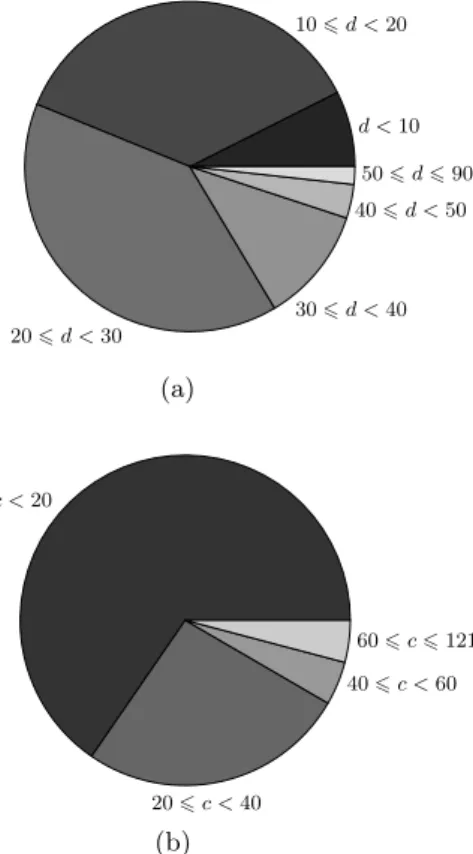
d < 10 10 6 d < 20 20 6 d < 30 30 6 d < 40 40 6 d < 50 50 6 d 6 90 (a) c < 20 20 6 c < 40 40 6 c < 60 60 6 c 6 121 (b)
Figure 2: Distributions of (a) degrees and (b) num-ber of critical points in our 650 examples.
software is Axel, [1] but no implementation of the certified subdivision algorithm is currentlty available.
Alcix is a C++ code, part of the CGAL library [10].6
Cad2d is a standalone C++ code which can also be com-piled in combination with the Singular library [26] (used for polynomial factorization). In our tests, Cad2d appears to be much more efficient when ran with Singular (and we re-port these tests). Finally, recall that Top requires an initial precision, which we set to 50.
As discussed in Section 1, the various implementations do not compute exactly the same thing and comparisons should thus be taken with care. Recall that when the curve is not in generic position, Top and Insulate do not compute the critical points (and, in particular, the x-extreme points) in the original coordinate system. isotop, Alcix and Cad2d always output the critical points in the original coordinate system.
We ran large scale benchmarks on over a thousand of curves during several weeks. In particular, we considered curves suggested in [30, 7, 25] and several classes of non-generic curves.7 We considered about 1300 curves from [30],
which are classified in 18 challenges covering a large variety
6Following the recommendation of M. Kerber,
we ran two versions of the code with the flag CGAL ACK RESULTANT FIRST STRATEGY set to 1 and 0. One being optimized for generic cases, while the other is optimized for singular curves. We always compare to the better running time.
7The logs are available at http://www.loria.fr/equipes/
vegas/isotop/benchmarks.
of interesting cases such as isolated points, high multiplic-ity of tangency at singularities, large number of branches at singularities or many singularities. This set contains curves of degree up 90 that are both in generic and non-generic position. As suggested in [7], typical curves in generic po-sition can be generated (i) as a random bivariate polyno-mial (which usually do not have singular points) or (ii) as resultants of two random trivariate polynomials (which usu-ally have singular points, including isolated points). In both cases, we considered random polynomials with 50% non-zero coefficients of bitsize 32 in Case (i) and initial bitsize 8 in Case (ii). We generated such curves with degrees up to 25. We also generated classes of curves in non-generic position in two different ways. First, we considered products of a curve with one or several of its vertical translates. Second, we considered curves of the type g = f2(x, y) + f2(x, −y);
such curves are usually irreducible and consist of isolated points which are the intersections of the curve Cf with its
symmetric with respect to the x-axis. We generated such curves with degrees up to 24.
We set in our experiments a limit of 30 minutes for the computation of the topology of one curve. We report as time out instances that exceed this running time. Also, Cad2d which uses Singular for modular arithmetic, often reports on difficult instances that the table of primes has been ex-hausted, which results in an interruption of computation; this is reported in the tables as aborted.
In summary, we ran our benchmarks on a total of 1500 curves. As mentioned above, it is not significant to compare C++ and Maple implementations when the running time is too small. We thus only report experiments on 650 curves whose running times exceeded 1 second for isotop. The distribution of degrees and number of critical points of these 650 curves is shown in Figure 2.
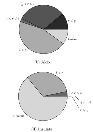
Figure 3 shows the ratio of running times between each of the competing implementations and isotop over our 650 curves. It appears difficult to analyze the benchmarks glob-ally because there are always particular examples that are processed faster by a given implementation. We note, how-ever, that Insulate is almost always slower than isotop, ex-cept for random curves with no singular points. In addition, Insulate and Top reached the time limit on more than half of the examples and, in particular, on difficult examples. We can, nevertheless, comment on the general behavior of the different approaches depending on the classes of examples.
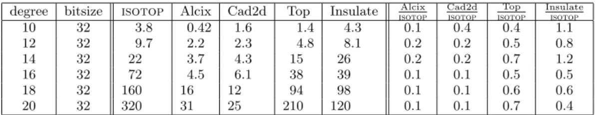
To illustrate the behavior on curves in generic positions, we report the running times for random curves in Table 1 and for resultants of surfaces in Table 2. Random curves have no singular points and few extreme points. In this case, we observe that isotop is the least efficient implementation. This can be explained by the fact that isotop computes the Gr¨obner basis of a large system without multiplicities, which is the worst case in practice. On the other hand, the other implementations benefit from interval arithmetic fil-ters in the lifting phase, which speed up computations by avoiding expensive symbolic computations, see for example [7]. Generic curves generated as resultants have many singu-larities and extreme points. isotop benefits from splitting the critical system in two smaller (singular and extreme) systems and hence it performs relatively better than in the completely random case. We observe that isotop is typi-cally a bit slower than Alcix but faster than Top, and that Cad2d aborts.
0 < r 61 3 1 3< r 6 1 1 < r 6 3 3 < r aborted (a) Cad2d r 61 3 1 3< r 6 1 1 < r 6 3 3 < r timeout (b) Alcix r 61 3 1 3< r 6 1 1 < r 6 3 3 < r timeout (c) Top r 61 3 1 3< r 6 1 1 < r 6 3 3 < r timeout (d) Insulate
Figure 3: Distributions of running time ratios for (a) Cad2d, (b) Alcix, (c) Top, and (d) Insulate over isotop. Timeout means that the limit of 30 minutes was reached.
To illustrate the behavior on curves in non-generic posi-tion, we consider different classes of curves. The first class of non-generic curves are constructed with one curve multiplied by one or several of its vertical translates. The initial curve is taken either randomly, in Table 3, or it is a resultant of two surfaces, in Table 4. Table 5 reports results on the second class of non-generic curves of the type f2(x, y) + f2(x, −y)
for random polynomials f . For these non-generic curves, isotop is typically faster than other implementations.
As a general rule, we observe that, except for random curves, that is, curves in generic position and without sin-gular point, the ratio of the running times between other implementations and isotop is increasing with the degree of the curve. In other words, except for random curves, iso-top tends to perform better, compared to others, when the degree increases.
6.
CONCLUSION
We presented a new algorithm and implementation for computing the topology of plane algebraic curves. Instead of a cylindrical algebraic decomposition based method, our algorithm relies upon Gr¨obner bases, Rational Univariate Representations and hence avoids computations with alge-braic numbers even in non-generic cases. A strength of our approach is to be insensitive to the non-genericity of the curve. As demonstrated by the experiments, our imple-mentation is competitive with state-of-the-art C/C++ im-plementations in the case of generic curves and faster for high-degree non-generic ones. Future work includes taking
advantage of the possible decomposition of the curve into factors. We already decompose the system of critical points into systems of extreme and singular points. One natural step further would be to consider the primary decompo-sitions of the ideals and thus work with systems of lower complexity.
Acknowledgments
We would like to thank the authors of Alcix, Cad2d, Insu-late, and Top for supplying their code and O. Labs for his list of curve challenges.
7.
REFERENCES
[1] L. Alberti, B. Mourrain, and J. Wintz. Topology and arrangement computation of semi-algebraic planar curves. Comput. Aided Geom. Des., 25(8):631–651, 2008. [2] D. Arnon and S. McCallum. A polynomial time algorithm
for the topological type of a real algebraic curve. J. Symbolic Computation, 5:213–236, 1988.
[3] D. S. Arnon, G. E. Collins, and S. McCallum. Cylindrical algebraic decomposition ii: An adjacency algorithm for the plane. SIAM J. Comput., 13(4):878–889, 1984.
[4] S. Basu, R. Pollack, and M.-R. Roy. Algorithms in Real Algebraic Geometry, volume 10 of Algorithms and
Computation in Mathematics. Springer-Verlag, 2nd edition, 2006.
[5] R. Benedetti and J. Risler. Real Algebraic and
Semi-algebraic Sets, Actualites Mathematiques. Hermann, 1990.
[6] C. W. Brown. Improved projection for cylindrical algebraic decomposition. J. Symb. Comput., 32(5):447–465, 2001.
degree bitsize isotop Alcix Cad2d Top Insulate Alcix isotop Cad2d isotop Top isotop Insulate isotop 10 32 3.8 0.42 1.6 1.4 4.3 0.1 0.4 0.4 1.1 12 32 9.7 2.2 2.3 4.8 8.1 0.2 0.2 0.5 0.8 14 32 22 3.7 4.3 15 26 0.2 0.2 0.7 1.2 16 32 72 4.5 6.1 38 39 0.1 0.1 0.5 0.5 18 32 160 16 12 94 98 0.1 0.1 0.6 0.6 20 32 320 31 25 210 120 0.1 0.1 0.7 0.4
Table 1: Running times in seconds (averaged over 5 runs) for random bivariate polynomials with 50% non-zero coefficients of bitsize 32.
degree bitsize isotop Alcix Cad2d Top Insulate Alcix isotop Cad2d isotop Top isotop Insulate isotop 16 64 29 14 aborted 52 >600 0.5 - 1.8 >20 25 80 590 410 aborted >1800 >1800 0.7 - >4.3 >3
Table 2: Running times (averaged over five runs) in seconds for resultants of two random trivariate polyno-mials, both of total degree 4 or 5, with 50% non-zero coefficients of bitsize 8.
degree τ isotop Alcix Cad2d Top Insulate Alcix isotop Cad2d isotop Top isotop Insulate isotop 12 96 4.1 6.5 1.6 9 or >600 >600 1.6 0.4 2.2 or >92 >140 15 96 15 38 10 40 or >600 >600 2.5 0.7 2.7 or >16 >40 18 96 49 120 66 >600 >600 2.4 1.3 > 12 >12 21 96 140 510 510 >1200 >1200 3.5 3.6 > 8.6 >9
Table 3: Running times (averaged over five runs) in seconds for non-generic curves generated by the product of a curve f with two of its translates f (x, y + 1) and f (x, y + 2). The curve f is chosen randomly with degree between 4 and 7 and 50% non-zero coefficients of bitsize 32, resulting in curves of bitsize τ . The running-time discrepancy of Top is large and is not averaged.
d1 d2 degree τ isotop Alcix Cad2d Top Insulate isotopAlcix Cad2disotop isotopTop Insulateisotop
3 3 18 96 26 93 160 >600 >600 3.6 6.3 >20 >20 3 4 24 112 250 510 or >1800 aborted >1800 >1800 2.0 or >7.2 - >20 >20 Table 4: Running times (averaged over five runs) in seconds for non-generic curves generated by the product of a curve f with its translate f (x, y + 1). The curve f is the resultant of two random trivariate polynomials of total degree d1 and d2 and 50% non-zero coefficients of bitsize 8. The running-time discrepancy of Alcix is
large for degree 24 and is not averaged.
degree bitsize isotop Alcix Cad2d Top Insulate Alcix isotop Cad2d isotop Top isotop Insulate isotop 10 64 39 180 25 >600 >600 4.5 0.6 >15 >15 12 64 240 300 aborted >1800 >1800 1.2 - >7 >7 14 64 350 >1800 aborted >1800 >1800 > 5 - >5 >5
Table 5: Running times (averaged over five runs) in seconds for polynomials of the form g = f2(x, y)+f2(x, −y). The random polynomials f have bitsize 32, term density 50% and degrees varying between 5 and 7.
[7] C. W. Brown. Contructing cylindrical algebraic decomposition of the plane quickly, 2002. Manuscript, http://www.cs.usna.edu/~wcbrown/.
[8] C. Burnikel, S. Funke, K. Mehlhorn, S. Schirra, and S. Schmitt. A separation bound for real algebraic expressions. In Proc. 9th Annual European Symposium on Algorithms, volume 2161 of LNCS, pages 254–265. Springer-Verlag, 2001.
[9] M. Burr, S.W.Choi, B. Galehouse, and C. Yap. Complete subdivision algorithms, ii: Isotopic meshing of singular algebraic curves. In Proc. Intl. Symp. on Symbolic & Algebraic Computation (ISSAC 2008), 2008.
[10] CGAL: Computational Geometry Algorithms Library. http://www.cgal.org.
[11] M. Coste and M. F. Roy. Thom’s lemma, the coding of real algebraic numbers and the computation of the topology of semi-algebraic sets. J. Symb. Comput., 5(1/2):121–129, 1988.
[12] D. Cox, J. Little, and D. O’Shea. Using Algebraic
Geometry. Number 185 in Graduate Texts in Mathematics. Springer, New York, 2nd edition, 2005.
[13] D. I. Diochnos, I. Z. Emiris, and E. P. Tsigaridas. On the complexity of real solving bivariate systems. In C. W. Brown, editor, Proc. Int. Symp. Symbolic and Algebraic Computation, pages 127–134, Waterloo, Canada, 2007. [14] A. Eigenwillig, M. Kerber, and N. Wolpert. Fast and exact
geometric analysis of real algebraic plane curves. In C. W. Brown, editor, Proc. Int. Symp. Symbolic and Algebraic Computation, pages 151–158, Waterloo, Canada, 2007. ACM.
[15] A. Eigenwillig, L. Kettner, W. Krandick, K. Mehlhorn, S. Schmitt, and N. Wolpert. A Descartes Algorithm for Polynomials with Bit-Stream Coefficients. In V. Ganzha, E. Mayr, and E. Vorozhtsov, editors, CASC, volume 3718 of LNCS, pages 138–149. Springer, 2005.
[16] A. Eigenwillig, V. Sharma, and C. K. Yap. Almost tight recursion tree bounds for the Descartes method. In Proc. Int. Symp. on Symbolic and Algebraic Computation, pages 71–78, New York, NY, USA, 2006. ACM Press.
[17] A. Eigenwilling and M. Kerber. Exact and efficient 2d-arrangements of arbitrary algebraic curves. In Proc. 19th Annual ACM-SIAM Symposium on Discrete
Algorithms (SODA08), pages 122–131, San Francisco, USA, January 2008. ACM-SIAM, ACM/SIAM.
[18] I. Z. Emiris, B. Mourrain, and E. P. Tsigaridas. Real Algebraic Numbers: Complexity Analysis and
Experimentation. In P. Hertling, C. Hoffmann, W. Luther, and N. Revol, editors, Reliable Implementations of Real Number Algorithms: Theory and Practice, volume 5045 of LNCS, pages 57–82. Springer Verlag, 2008. also available in www.inria.fr/rrrt/rr-5897.html.
[19] J.-C. Faug`ere. A new efficient algorithm for computing gr¨obner bases without reduction to zero f5. In
International Symposium on Symbolic and Algebraic Computation Symposium - ISSAC 2002, Villeneuve d’Ascq, France, Jul 2002.
[20] H. Feng. Decomposition and Computation of the Topology of Plane Real Algebraic Curves. Ph.d. thesis, The Royal Institute of Technology, Stockholm, 1992.
[21] FGb - A software for computing Gr¨obner bases. J.-C. Faug`ere. http://fgbrs.lip6.fr.
[22] M. Giusti, G. Lecerf, and B. Salvy. A Gr¨obner free alternative for solving polynomial systems. J. of Complexity, 17(1):154–211, 2001.
[23] L. Gonz´alez-Vega and M. El Kahoui. An improved upper complexity bound for the topology computation of a real algebraic plane curve. J. Complexity, 12(4):527–544, 1996. [24] L. Gonz´alez-Vega, H. Lombardi, T. Recio, and M.-F. Roy. Sturm-Habicht Sequence. In Proc. Int. Symp. on Symbolic and Algebraic Computation, pages 136–146, 1989. [25] L. Gonz´alez-Vega and I. Necula. Efficient topology
determination of implicitly defined algebraic plane curves. Computer Aided Geometric Design, 19(9), 2002.
[26] G.-M. Greuel, G. Pfister, and H. Sch¨onemann. Singular 3.0 — a computer algebra system for polynomial computations. In M. Kerber and M. Kohlhase, editors, Symbolic computation and automated reasoning, The Calculemus-2000 Symposium, pages 227–233. A. K. Peters, Ltd., Natick, MA, USA, 2001.
[27] H. Hong. An efficient method for analyzing the topology of plane real algebraic curves. Mathematics and Computers in Simulation, 42(4–6):571–582, 1996.
[28] M. Kerber. Analysis of real algebraic plane curves. Master’s thesis, MPII, 2006.
[29] J. Keyser, K. Ouchi, and M. Rojas. The exact rational univariate representation for detecting degeneracies. In DIMACS Series in Discrete Mathematics and Theoretical Computer Science. AMS Press, 2005.
[30] O. Labs. A list of challenges for real algebraic plane curve visualization software. Manuscript, 2008.
[31] C. Li, S. Pion, and C. Yap. Recent progress in exact geometric computation. J. of Logic and Algebraic Programming, 64(1):85–111, 2004. Special issue on“Practical Development of Exact Real Number Computation”.
[32] S. McCallum and G. E. Collins. Local box adjacency algorithms for cylindrical algebraic decompositions. J. Symb. Comput., 33(3):321–342, 2002.
[33] B. Mourrain, S. Pion, S. Schmitt, J.-P. T´ecourt, E. P. Tsigaridas, and N. Wolpert. Algebraic issues in Computational Geometry. In J.-D. Boissonnat and M. Teillaud, editors, Effective Computational Geometry for Curves and Surfaces, Mathematics and Visualization, chapter 3. Springer, 2006.
[34] B. Mourrain and P. Tr´ebuchet. Generalized normal forms and polynomial system solving. In Proc. Int. Symp. Symbolic and Algebraic Computation, pages 253–260, 2005. [35] F. Rouillier. Solving zero-dimensional systems through the
rational univariate representation. J. of Applicable Algebra in Engineering, Communication and Computing,
9(5):433–461, 1999.
[36] F. Rouillier and P. Zimmermann. Efficient isolation of polynomial real roots. J. of Computational and Applied Mathematics, 162(1):33–50, 2003.
[37] RS - A software for real solving of algebraic systems. F. Rouillier. http://fgbrs.lip6.fr.
[38] T. Sakkalis. The topological configuration of a real algebraic curve. Bull. Austrl. Math. Soc., 43:37–50, 1991. [39] T. Sakkalis and R. Farouki. Singular points of algebraic
curves. J. Symb. Comput., 9(4):405–421, 1990.
[40] R. Seidel and N. Wolpert. On the exact computation of the topology of real algebraic curves. In Proc 21st ACM Symposium on Computational Geometry, pages 107–115, 2005.
[41] A. Strzebonski. Cylindrical algebraic decomposition using validated numerics. J. Symb. Comput., 41(9):1021–1038, 2006.
[42] B. Teissier. Cycles ´evanescents, sections planes et
conditions de Whitney. (french). In Singularit´es `a Carg`ese (Rencontre Singularit´es G´eom. Anal., Inst. ´Etudes Sci., Carg`ese, 1972), number 7–8 in Asterisque, pages 285–362. Soc. Math. France, Paris, 1973.