Influence of weather and global warming in chloride ingress into concrete: a stochastic approach

HAL Id: hal-00796726

https://hal.archives-ouvertes.fr/hal-00796726

Submitted on 4 Mar 2013

HAL is a multi-disciplinary open access

archive for the deposit and dissemination of

sci-entific research documents, whether they are

pub-lished or not. The documents may come from

teaching and research institutions in France or

abroad, or from public or private research centers.

L’archive ouverte pluridisciplinaire HAL, est

destinée au dépôt et à la diffusion de documents

scientifiques de niveau recherche, publiés ou non,

émanant des établissements d’enseignement et de

recherche français ou étrangers, des laboratoires

publics ou privés.

Influence of weather and global warming in chloride

ingress into concrete: a stochastic approach

Emilio Bastidas-Arteaga, Alaa Chateauneuf, Mauricio Sánchez-Silva, Philippe

Bressolette, Franck Schoefs

To cite this version:

Emilio Bastidas-Arteaga, Alaa Chateauneuf, Mauricio Sánchez-Silva, Philippe Bressolette, Franck

Schoefs. Influence of weather and global warming in chloride ingress into concrete: a stochastic

approach. Structural Safety, Elsevier, 2010, 32 (4), pp.238-249. �10.1016/j.strusafe.2010.03.002�.

�hal-00796726�

Influence of weather and global warming in chloride ingress into concrete: a

stochastic approach

E. Bastidas-Arteagaa,b_{, A. Chateauneuf}c_{, M. S´anchez-Silva}a_{, Ph. Bressolette}c_{, F. Schoefs}b

a

Department of Civil and Environmental Engineering. Universidad de los Andes, Carrera 1 E. 19A-40 Edificio Mario Laserna. Bogot´a, Colombia

b

GeM, UMR 6183 – University of Nantes, BP 92208 - 44322 Nantes cedex 3, France

c

LaMI – Blaise Pascal University, BP 206 - 63174 Aubi`ere cedex, France

Abstract

Reinforced concrete (RC) structures are subject to environmental actions affecting their performance, serviceability and safety. Among these actions, chloride ingress leads to corrosion and has been recognized as a critical factor reducing the service life of RC structures. This paper presents a stochastic approach to study the influence of weather conditions and global warming on chloride ingress into concrete. The assessment of chloride ingress is carried out on the basis of a comprehensive model that couples the effects of convection, chloride binding, concrete aging, temperature and humidity. A simplified model of temperature and humidity including seasonal variations and global warming is also proposed in this work. Three scenarios of global warming are defined based on: gas emissions, global population growth, introduction of new and clean technologies and use of fossil sources of energy. The proposed approach is illustrated by a numerical example where it is found that the climate changes may yield to significant lifetime reductions. These results justify the implementation of countermeasures directed to (1) reduce and/or mitigate the action of global warming on weather and (2) minimize the impact of climate changes on RC structures.

Key words:

Global warming, stochastic modeling, reliability, chloride ingress, corrosion, reinforced concrete

1. Introduction

During their operational life, reinforced concrete (RC) structures are subject to external actions affecting its performance, serviceability and safety [1]. External actions are divided into operational and environmen-tal. Operational deterioration results from the existence and the use of the structure (e.g., service loading, storage of chemical or biological products, etc.). Environmental deterioration is induced by the conditions of the surrounding environment (e.g., temperature, humidity, carbonation, chloride ingress, biodeterioration, etc.). The main effect of the combined action of operational and environmental demands on RC structures is a loss of resistance due to corrosion. The RC structures are susceptible to corrosion when they are placed in atmospheres with high concentrations of chloride ions or carbon dioxide. Corrosion induced by chloride ingress has been recognized as an important factor reducing the service life of RC structures. According to Bhide [2], about 173,000 bridges on the interstate system of the United States are structurally deficient or functionally obsolete due in part to corrosion.

At the beginning of the service life, a thin passive layer of corrosion products protects the steel rein-forcement against corrosion. Nevertheless, corrosion begins when the concentration of chlorides at the steel surface reaches a threshold value destroying the passive protective layer. Corrosion affects the load carrying capacity of structures by different mechanisms: loss of reinforcement cross-section, loss of steel-concrete bond, concrete cracking and delamination. Therefore, understanding the mechanisms and kinematics of corrosion have formed a basis for making quantitative predictions of the service life of RC structures.

Chloride ingress into concrete matrix is dominated by a complex interaction between physical and chem-ical processes. According to Tuutti [3], the diffusion problem can be represented by Fick’s second law under

the following assumptions: (1) concrete homogeneity, (2) constant chloride diffusion coefficient (in time and space), (3) chloride flow in saturated conditions, and (4) constant chloride concentration at the exposed concrete surface. Although closed-form solutions of Fick’s second law can be obtained, they cannot repre-sent accurately real structural deterioration processes, leading to poor predictions. Other factors affecting the chloride ingress phenomenon are chloride binding, concrete aging, interaction with temperature and humidity, etc. Saetta et al. [4] and latter Mart´ın-P´erez et al. [5] have proposed some strategies to account for such factors.

Experimental evidence indicates that the chloride ingress is highly influenced by the weather conditions at the surrounding environment. Bastidas-Arteaga et al. [6] found that accounting for the time-variant nature of humidity and temperature influences significantly the time to corrosion initiation. Thus, since studies on global warming have predicted several changes in the climate, their impact on structural reliability should be also considered. Global warming refers to the effect of human activities on weather; namely, the burning of fossil fuels (coal, oil and gas) and large-scale deforestation cause emissions to the atmosphere of greenhouse gases of which the most important is carbon dioxide [7]. As a result of these emissions, changes in climate are expected, affecting human communities and ecosystems –i.e., sea-level rise, increase in frequency and intensity of many extreme climate events, more frequent heat waves, increases in rainfall, etc. The society should be aware of this problem and adopt countermeasures to mitigate and to face up to these changes. From an engineering point of view, the impact of climate change on the performance of structures should be seriously studied.

Given that substantial uncertainties cannot be neglected in this problem, a probabilistic framework becomes paramount for appropriate lifetime assessment. The sources of randomness are related to: (1) RC material properties, (2) quality of mechanical models and their parameters, and (3) prediction and assessment of environmental conditions. Several works have integrated probabilistic methods for lifetime prediction of deteriorating RC structures including the coupled action of various deterioration processes [8, 9]. Regarding to chloride flow into concrete, Kong et al. [10] performed a reliability analysis that mainly accounted for the uncertainties related to the material properties. However, the proposed methodology was only applied to saturated concrete. The effect of two-dimensional modeling of chloride ingress on the probabilistic evaluation of the corrosion initiation time was studied by Val and Trapper [11]. This work took into account the model presented in [4, 5] to perform a probabilistic evaluation of the corrosion initiation time. Although the chloride flow in unsaturated concrete is taken into account, it does not considered the heat flow into the concrete and the impact of the stochastic nature of humidity and temperature in the corrosion initiation time assessment. These points were addressed in a recent work carried out by the authors [6], where the factors controlling the chloride ingress and the effect of weather conditions were accounted for.

In order to study the chloride ingress from an integral perspective, the goals of the present work are to: • introduce a comprehensive model of chloride ingress that accounts for: (1) chloride binding capacity, (2) time-variant nature and the effects of temperature, humidity and chloride concentration at the surrounding environment, (3) decrease of the chloride diffusivity with aging and (4) chloride flow in unsaturated concrete;

• consider a weather model that considers the random nature of the parameters including the effects of global warming; and

• integrate the model of chloride ingress into a probabilistic framework to take into account the ran-domness related to the phenomena.

Section 2 summarizes the implemented model of chloride penetration and its solution procedure. The proposed weather model which includes global warming is presented in section 3. Section 4 presents the adopted stochastic approach to the problem. Finally, a numerical example is presented in section 5.

2. Modeling chloride penetration

2.1. Governing equations of chloride penetration

A comprehensive model for chloride ingress into concrete must account for: influence of temperature and humidity, temporal variation of the surface chloride concentration, concrete aging, chloride ingress by convection and chloride binding. This section presents the formulation applied to manage the interaction between the three phenomena:

1. chloride ingress, 2. moisture diffusion and 3. heat transfer,

Each phenomenon is represented by a partial differential equation (PDE) and the interaction between these three phenomena is considered by solving simultaneously a coupled system of PDEs. According to Mart´ın-P´erez et al [5], the governing equations of the phenomena can be expressed in the following general form: ζ∂ψ ∂t = div J| {z } diffusion + div J0 | {z } convection (1)

where ψ represents the parameter under consideration (e.g., chloride ions, moisture, heat), t is the time and

the terms ζ, J, J0 _{depend on the physical problem as presented in Table 1.}

For chloride ingress, Eq. 1 becomes: ∂Cf c ∂t = div ⇣ D⇤c − ! r (Cf c) ⌘ | {z } diffusion + div⇣Cf cD⇤h − ! r (h)⌘ | {z } convection (2)

where Cf c is the concentration of free chlorides, h is the relative humidity and D⇤c and Dh⇤ represent the

apparent chloride and humidity diffusion coefficients, respectively [4]: Dc⇤= Dc,ref f1(T )f2(t)f3(h) 1 + (1/we) (∂Cbc/∂Cf c) (3) D⇤h= Dh,ref g1(h)g2(T )g3(te) 1 + (1/we) (∂Cbc/∂Cf c) (4)

where Dc,ref and Dh,ref are reference diffusion coefficients measured in standard conditions [4], we is the

evaporable water content, and fi and gi are correction functions to account for the effects of temperature

T , relative humidity h, aging t and hydration (curing) period te. These functions are detailed in appendix

A. The term ∂Cbc/∂Cf c represents the binding capacity of the cementitious system which relates free and

bond chlorides concentration at equilibrium [12]. Langmuir and Freundlich isotherms are the most used to estimate the binding capacity [13, 14]. Taking into account that both isotherms provide very close solutions when the isotherm parameters correspond to the same concrete [6] and that Glass and Buenfeld found that chloride binding is estimated more accurately by Langmuir isotherm [14], such isotherm is used in this work:

CbcL =

αLCf c

1 + βLCf c

(5)

where αL and βL are binding coefficients obtained experimentally which depend on cement properties;

mainly, the content of tricalcium aluminate C3A. For instance, for a medium content of 8% of C3A these

coefficients are αL= 0.1185 and βL= 0.090 [14].

For moisture diffusion, the substitution of the terms presented in Table 1 into Eq. 1 gives:

∂we ∂t = ∂we ∂h ∂h ∂t = div ⇣ Dh − ! r (h)⌘ (6)

where the diffusion coefficient Dh depends mainly on humidity, temperature and hydration period –i.e.,

Dh= Dh,refg1(h)g2(T )g3(te). The correction functions used to account for the influence of such parameters,

gi, are also presented in appendix A. The term ∂we/∂h represents the moisture capacity which relates the

amount of free water, we, and the pore relative humidity, h. For a given temperature this relationship has

been determined experimentally by adsorption isotherms. According to the Brunauer-Skalny-Bodor (BSB) model, the adsorption isotherm can be estimated as [15]:

we=

CkVmh

(1 − kh) [1 + (C − 1) kh] (7)

where the parameters C, k and Vm depend on temperature, water/cement ratio, w/c, and the hydration

period, te. The present work considers the empirical expressions of Xi et al. [16] for such parameters; for

instance, for te≥ 5 days, 0.3 < w/c  0.7 and for ordinary Portland cement:

C = exp(855/T ) (8)

k = (1 − 1/nw) C − 1

C − 1 (9)

nw= (2.5 + 15/te) (0.33 + 2.2w/c) (10)

Vm= (0.068 − 0.22/te) (0.85 + 0.45w/c) (11)

Finally, the governing equation for heat transfer is: ρccq∂T

∂t = div

⇣

λ−!r (T )⌘ (12)

where ρc is the concrete density, cq is the concrete specific heat capacity, λ is the thermal conductivity of

concrete and T is the temperature inside the concrete matrix after time t. For ordinary Portland concrete,

Neville [17] reports that cq varies between 840 and 1170 J/(kg oC) and λ between 1.4 and 3.6 W/(moC).

The coupling between the tree phenomena can be summarized as follows: the solution of the heat transfer is essential to determine the moisture diffusion; afterwards, both results (temperature and moisture) are necessary to estimate chloride ingress. Since the coupled system of PDEs has a similar form (Eq. 1), it is possible to adopt the same numerical tool to solve the whole system. Section 2.2 describes the numerical approach used in this study.

2.2. Numerical solution of the governing equations

To determinate the profiles of chlorides, humidity and temperature into the concrete during the exposure time, it is necessary to solve simultaneously the system of PDEs described in section 2.1. For this purpose, finite element and finite difference methods are combined. Whereas the spatial variation of ψ throughout the considered mesh is computed by the finite element method, its evolution in time is integrated by using the finite difference Crank-Nicolson method.

The algorithm to determine the profiles of temperature, humidity and chlorides (considering unidirec-tional flow –e.g., x), is presented in Figure 1. At the beginning, initial values of ψ are fixed for the mesh

–i.e., Tini, hini and Cf c,ini. For new structures, these values can be defined, for instance, by taking into

consideration the concrete properties at the end of construction. However, for chloride-contaminated struc-tures, the measured profile of chlorides could be included as the initial profile. By accounting for the profile

of ψ corresponding to a previous time-step e.g. t = ti− ∆t, the procedure to determinate the actual profile

of ψ at t = ti is:

1. the actual temperature profile is determined from the governing equation of heat transfer by considering

the initial temperature profile Tini= T (x; ti−1);

2. with the temperature profile estimated in the previous step and the initial humidity profile hini =

h(x; ti−1), the actual humidity profile is determined from the moisture diffusion relationship; and

3. the profile of chlorides is found from the chloride ingress equation by accounting for the actual profiles

of temperature and humidity, and the initial values of free chlorides Cf c,ini= Cf c(x; ti−1).

These steps are repeated for the next time-step by setting the actual profiles as initial values. Since equations of chloride ingress and moisture diffusion are nonlinear, it is necessary to implement an iterative procedure to estimate the profiles of chlorides and humidity. This nonlinearity comes from the dependence of the diffusion coefficients and isotherms on the actual profiles of humidity and chlorides. A detailed explanation of the solution methodology is presented in [5].

The boundary conditions at the exposed surfaces consider the flux of ψ crossing the concrete surface, qs

ψ

(Robin boundary condition) [4]: qsψ= Bψ(ψs− ψenv) | {z } diffusion + ψenvqψ0s | {z } convection (13)

where Bψ is the surface transfer coefficient, ψsis the value of ψ at the exposed surface and ψenv represents

the value of ψ in the surrounding environment for each physical problem. The terms in Eq. 13 are also

presented in Table 1. By fitting experimental data, Saetta et al. [4] reported that BCf c varies between 1

and 6 m/s. Typical values of Bh are in the range of 2.43 − 4.17 ⇥ 10−7 m/s [18]. Finally, Khan et al. [19]

observed that BT fluctuates between 6.2 and 9.3 W/(m2oC).

3. Modeling weather including warming effects

Weather measurements on global warming anticipate changes in the mean temperature and humidity in the coming years [20]. It has been found that eleven of the twelve years of the period (1995–2006) rank among the warmest years since the beginning of the instrumental record of global surface in 1850. Besides,

the linear warming trend over the last 50 years (0.13o_{C per decade) almost doubles the measurements during}

the last 100 years (0.076o_{C). Based on these measurements and different policies against global warming, the}

Intergovernmental Panel on Climate Change announces a raise from 1 to 6.4o_{C for the following 100 years.}

The basic science of weather modeling, including the greenhouse effect, is well understood and has been discussed widely. Most of these models demand large computational efforts because they integrate dynamical and physical equations to describe the complete climate system [7]. Nowadays, about fifteen research centers in the world are running fully coupled models. Given the difficulties to integrate a comprehensive weather model with the chloride ingress phenomenon, a simplified model of global warming is presented in this section. It accounts for the following aspects:

• influence of global warming,

• seasonal variation of weather parameters, and • random nature of weather.

The effect of global warming is modeled by assuming a linear variation of the weather parameters; while the seasonal variations of the parameters follow a sinusoidal shape. The uncertainties related to weather are treated in section 4.

3.1. Mean trend of global warming and seasonal variation

The increase or decrease of temperature and humidity for the upcoming years are modeled by a linear time-variant function. By denoting φ as the weather parameter (humidity or temperature), the annual mean value of φ is equal to (Figure 2):

¯ φ(t) = ¯φ0+ ✓ ¯_φt a− ¯φ0 ta ◆ t (14)

where ¯φ0 and ¯φta are the values of the annual means of φ at t = 0 and t = ta, respectively. On the other

seasonal variations of humidity and temperature during the year (Figure 2). The model divides a reference year into two seasons hot and cold for the temperature, and wet and dry for the humidity. Actual forecasts

of global warming also indicate that the droughts increase the length of hot (or wet) seasons, Lh, with

respect to the length of cold (or dry) seasons, Lc [20]. By defining R0 as the normalized duration of the

cold (or dry) season for t = 0, i.e. R0= Lc/ 1 year, and Rta as the normalized duration of the cold or dry

season for t = ta (Lc in years); it is possible to estimate linearly the normalized duration of the cold or dry

season R for a given t:

R(t) = R0+

✓ Rta− R0

ta

◆

t (15)

Thus by using a sinusoidal formulation to simulate the seasonal variation of φ around the linear trend (Eq. 14), the seasonal mean of φ becomes (Figure 2):

¯ κ(t) = 8 < : ¯ φ(t) +φmax−φmin 2 sin ⇣ _t−btc 1−R(t)π ⌘

for the hot or wet seasons ¯ φ(t) −φmax−φmin 2 sin ⇣_{t−btc+R(t)−1} R(t) π ⌘

for the cold or dry seasons (16)

where φmax and φmin are respectively the maximum and minimum values taken by φ during one year, t is

expressed in years and b·c represents the floor function –i.e., bxc = max {n 2 Z | n  x}. 3.2. Selected scenarios

Three possible scenarios of global warming were defined in this work. The characteristic of these sce-narios were defined based on the forecasts given in the report of the Intergovernmental Panel on Climate Change [20]; which to the authors’ opinion, presents the most compendious work in global warming. These predictions account for a combination of natural and anthropogenic forcings. The action of natural forcings refer to natural climate changes due mainly to solar and volcanic activities. Anthropogenic forcings encom-pass the effect of human perturbations on climate. Among the anthropogenic forcings, the most important factors considered in such study are:

• carbon dioxide, methane, nitrous oxide emissions; • global population growth;

• introduction of new and clean technologies leading to reduce the impact of global change and • use of fossil sources of energy.

Consequently, the three possible scenarios are without, expected and pessimistic global warming. Each scenario is defined in terms of:

• the difference between the annual means of temperature for the initial year t0and the year of the end

of the forecast ta, ∆Ta = Tta− Tt0,

• the difference between the annual mean of relative humidity for t0and ta, ∆ha = hta− ht0, and

• the difference between the normalized durations of the cold seasons for t0 and ta, ∆Ra= Rta− Rt0.

By taking as reference a period of analysis of 100 years –i.e., ta= 100 years, the features and the values of

∆Ta, ∆haand ∆Rafor each scenario are presented in Table 2. Figure 3 shows an example of the temperature

model including the effects of global warming. For seasonal variation, the temperature fluctuates between

Tmin = −10oC and Tmax = 20oC for a year. Taking into consideration all scenarios of global warming

described in Table 2, the impact of climate change at the end of the reference period is easily observable.

Namely, the length of the cold seasons has decreased –i.e., R0> Rta, and the temperatures during the whole

year are higher. This difference is emphasized for the pessimistic scenario. Although in general terms the presented model simulates the effect of seasonal variations and global warming on temperature and humidity,

it is important to stress that predicted values only represent an overall behavior which does not includes the randomness of the phenomena. Therefore, the proposed model of global warming will be coupled with stochastic processes to enhance its predictability. This improvement allows considering the appearance of hotter and colder periods and extreme values during the period of analysis. This and other random aspects will be addressed in following section.

4. Uncertainty modeling

In order to perform appropriate predictions of structural lifetime, the uncertainties related to the problem should be integrated in the analysis. The sources of randomness involved in this problem are associated to:

• the environmental actions; • the material properties; and • the model parameters.

This work considers the environmental actions as stochastic processes to account for the time-dependency on weather parameters and chloride concentration at the surface. The uncertainties related to concrete properties and model parameters are taken into account by considering the main variables as random variables characterized by appropriated probability distributions. The following subsections describe the adopted stochastic models as well as the probabilistic analysis scheme.

4.1. Weather modeling

Given that chloride penetration is highly dependent on weather conditions, it is necessary to implement a model that accounts for seasonal variations as well as for the effects of global warming. The stochastic processes are valuable tools to discretize the problem. Karhunen-Lo`eve expansions or polynomial chaos are two rational methodologies to deal with this problem [21]. However, due to both simplicity of implementation and computational time, this study only implements Karhunen-Lo`eve expansions to model humidity and temperature. The discretization by Karhunen-Lo`eve expansion is based on the spectral decomposition of

the covariance function of the process C(t1, t2) and consists in representing a random process κ(t, θ) by a

combination of orthogonal functions fi(t) on a bounded interval –i.e. [−a, a]. If κ(t, θ) is defined over the

domain D, with θ belonging to the space of random events Ω, κ(t, θ) is expanded as [21]:

κ (t, θ) ' ¯κ(t) + nkl X i=1 p λiξi(θ)fi(t) (17)

where ¯κ(t) is the mean of the process, ξi(θ) is a set of standard Gaussian variables, nkl is the number of

terms of the truncated discretization and λiare the eigenvalues of the covariance function C(t1, t2) resulting

from the evaluation of the following expression: Z

D

C(t1, t2)fi(t2)dt2= λifi(t1) (18)

The solution of Equation 18, can be analytically determined when the covariance function is exponential or triangular. For both weather models this study assumes an exponential covariance:

C(t1, t2) = e−|t1−t2|/b (19)

where b is the correlation length and must be expressed in the same units of t. The expressions to compute

fi(t) and λi obtained for the exponential covariance are detailed in [21]. On the other hand, the mean of the

stochastic process ¯κ is modeled as a deterministic time-variant function which considers the effects of global

representing temperature where the parameters for the time-variant mean are T0 = 5oC, Tta = 7.5

o_C,

Tmin = −10oC, Tmax = 20oC, ta = 100 years, R0 = 0.5 and Rta = 0.4. These values will be used in

section 5 for characterization of the continental environment. From the comparison between time-variant and stochastic modeling it is important to stress that although the stochastic realization follows the tendency of the time-variant mean, it includes the appearance extreme values during the exposure time. This behavior has been observed for real exposure conditions.

4.2. Modeling of surface chloride concentration

The chloride ions that ingress into the concrete can come from two sources: sea or de-icing salts. This section presents the stochastic models used to simulate the chloride concentration in both environments. 4.2.1. Exposure to chlorides from sea water

For this type of exposure, the surface chloride concentration depends principally on the closeness to the sea, d. Based on a field study of 1158 bridges in Australia [22], the mean of the surface chloride concentration,

µCenv, can be computed as:

µCenv(d) = 8 < : 2.95 for d < 0.1 1.15 − 1.81 log(d) for 0.1  d < 2.84 0.35 for d > 2.84 (20)

where d is expressed in km and µCenv in kg/m

3_.

By taking the values of Eq. 20 as mean, the stochastic process representing Cenv is generated with

uncorrelated log-normal noise. It is worthy to precise that for both exposures (sea and de-icing salts) the models of surface chloride concentration represent environmental chloride concentrations and not notional surface concentrations (which appears from empirical models based on the solution of Fick’s law) [11]. Since there is no information available about the coefficient of variation (COV) for environmental chloride concentrations, the COV used herein is based on previous probabilistic studies which consider notional

surface concentrations [23, 24]. Figure 5a presents some realizations of Cencwhere the processes are generated

by considering three values of µCenv: 2.95, 1.15 and 0.35 kg/m

3 _{which correspond to d < 0.1, d = 1 and}

d = 2.84 km, respectively (equation 20); a COV of 0.20 was used for all these cases. 4.2.2. Exposure to chlorides from de-icing salts

The second type of exposure encompasses structures regularly subject to de-icing salts during winter. Based on experimental measurements, the probabilistic models of exposure to de-icing salts in the literature

usually assume that Cenv remains constant during all time [23, 24]. However, since the kinematics of the

chloride ingress change as function of the weather conditions, a modified model for de-icing salts exposure

is adopted. This model considers the increase of Cenv during the cold seasons. Thus, the proposed model

assumes that during the hot seasons the mean of chloride concentration at the surface be zero, whereas

during the cold seasons it varies as a linear function from zero until a maximum, Cmax

env , that corresponds

to the minimum temperature and returns to zero at the beginning of the hot season (Figure 5b):

µCenv(t) = 8 < : 0 for t < t1 Cmax env (t − t1)/(t2− t1) for t1 t < t2 Cmax env [1 − (t − t2)/(t2− t1)] for t2 t < t3 (21)

where t1, t2 and t3 are shown in Figure 5b. The value of Cenvmax has been defined by considering that the

quantity of chloride ions deposited during one year be the same that the average annual concentration

reported in the literature, Cave

env. It is important to observe that the mean of Cenv should be coupled to the

effect of global warming because the decrease of the length of cold seasons Lcwill reduce the use of de-icing

salts. Therefore the values of t1, t2and t3 are computed and adjusted year by year by using the normalized

duration of the cold season –i.e., Eq. 15.

The stochastic model for de-icing exposure establishes that Cenv is zero during the hot season and

computed from Eq. 21 and the COV should be assumed until actual data be acquired. An example of the

stochastic modeling of Cenv for de-icing exposure is also presented in Figure 5a. The maximum surface

chloride concentration, Cmax

env , is equal to 14 kg/m3. This value assures that the mean of the chloride ions

deposited during a year be 3.5 kg/m3 _{agreeing with the data reported in [23, 24]. A COV of 0.20 was used}

to generate the process.

4.3. Probability of corrosion initiation

To account for randomness, the mechanical model described in the previous sections is integrated with an appropriate reliability approach that gives as result the probability of occurrence of a given event. The

focus on this study is put on the time to corrosion initiation, tini, which occurs when the concentration of

chlorides at the cover thickness ctis equal to or higher than a threshold value Cth. For such event, the limit

state function can be written: g(x

¯,t) = Cth(x¯) − Ctc(x¯,t, ct) (22)

where x

¯ is the vector of the random variables to be taken into account and Ctc(x¯,t, ct) is the total

concen-tration of chlorides at depth ctand time t. By evaluating the limit state function (Eq. 22), the probability

of corrosion initiation is:

pcorr(t) = P[g(x

¯,t)  0|t] (23)

The probability of corrosion initiation is obtained by computing the chloride concentration at the cover depth from the solution of the system of PDEs presented in section 2. Given the complexity of the solution of the system of PDEs, simulation methods seem to be appropriate to deal with the problem. Therefore this study combines Monte Carlo simulations with Latin Hypercube Sampling to reduce the computational cost.

5. Illustrative example 5.1. Definition of the study case

The main goal of this example is to study the influence of real weather conditions on both the probability of corrosion initiation and the lifetime reduction. To this aim, let us consider a RC slab or wall, with a side exposed to environmental actions (Figure 6a). Knowing that the depth of the RC member is much smaller than their other dimensions, the problem is reduced to one-dimensional flow of chlorides into concrete. However, it is worthy to highlight that for smaller members (e.g., columns or beams) the two-dimensional flow accelerates the corrosion initiation for the corner bars [6, 11].

This application accounts for three environments with the characteristics defined by both the site latitude and closeness to the sea. Table 3 describes and presents the values adopted for each climate case. To account for the effect of global warming, the three scenarios described in Table 2 are also included in the analysis. Other assumptions in this example are:

• the concentration of chlorides inside the concrete is zero at the begin of the analysis; • the structure is located in a partially-saturated media;

• the considered concrete contains 400 kg/m3 _{of ordinary Portland cement, 8% of C}

3A and w/c = 0.5;

• the hydration period, te, is 28 days (see Eq. 29, Appendix A);

• the COV of the environmental chloride concentration is 0.2; and • the random variables are independent.

The probabilistic models of the random variables used in this example are shown in Table 4. For

chloride ingress, the mean of the reference chloride diffusion coefficient, Dc,ref, is assigned according to the

experimental values presented in [4] for w/c = 0.5. Both the probabilistic model and the COV of Dc,ref

follow the suggested in [11, 24]. By defining Cthas the critical chloride content which leads to deterioration

or damage of a concrete member located in an environment constantly humid, the statistical parameters

of Cth are defined by the values reported in [24]. According to [23, 24], the cover thickness, ct, follows a

truncated normal distribution with the mean and COV indicated in Table 4. Based on experimental studies

[25], it is supposed that the activation energy of the chloride diffusion process, Uc, (see appendix A) follows

a beta distribution with the values presented in Table 4. The age reduction factor, m, also follows a beta

distribution [26]. For moisture diffusion, The reference humidity diffusion coefficient, Dh,ref, is log-normally

distributed with a mean and COV defined on the basis of [4, 11, 24]. It is also supposed that the parameters

α0 and n (appendix A) follow a beta distribution which statistical parameters are defined according to

experimental studies [27, 28]. For heat transfer, the thermal conductivity of concrete λ and the concrete

specific heat capacity cq, follow beta distributions with the means reported by [17] and vary between the

bounds established experimentally. Taking as mean the typical density of normal concrete, it is assumed that this variable is normally distributed with a COV of 0.2.

5.2. Results and comments

For a better understanding of the effects of global warming on RC structures under real weather condi-tions, this section distinguish between two main issues:

• the probability of corrosion initiation without climate changes, and • the lifetime reduction induced by global warming.

The results presented herein also account for: the stochastic model of humidity and temperature, chlo-ride binding (Langmuir isotherm) and convection. Whereas for the continental environment, the chlochlo-ride

concentration is Cmax

env = 14 kg/m3 , for the marine environment, it depends on the distance from the sea

–i.e., Eq. 20.

5.2.1. Probability of corrosion initiation without climate changes

The aim of this analysis is to perform a comprehensive study of the influence of weather conditions without considering the climate change repercussions. This study includes the effects of:

• three different environmental exposures (continental, tropical and oceanic) and

• the distance to the sea d (less than 100 m, around 1 km or more than 3 km) for marine environments. The effect of the type of environmental exposure on the probability of corrosion initiation is plotted in Figure 6b. This Figure presents the probabilities of corrosion initiation for the environments described in Table 3. The surface chloride concentration for the marine environment (tropical or oceanic), is defined

by a distance to the sea d < 0.1km. It is observed at each time that the highest pcorr corresponds to

the marine environments, in particular, for the tropical environment. These results are explained by the facts that (1) structures placed in marine environments are exposed to chlorides all the time and (2) higher temperature and humidity accelerate the penetration of chloride ions inside the concrete matrix. The difference between the continental and the tropical environments highlights the importance of implementing a chloride penetration model that includes the environmental effects. Namely, given that the environmental chloride concentration is the same for both marine environments, a simplified analysis would lead to the same results for the both environments when climatic considerations are not taken into account.

Figure 7 describes the influence of the distance from the sea on the probability of corrosion initiation. These profiles were computed for the oceanic and tropical environments. It is observed that the probability of corrosion initiation is bigger for the nearest places to the sea. This behavior is due to the increase of the environmental chloride concentration when the distance to the sea d is reduced (Eq. 20). The impact of the distance of the sea can be observed by analyzing the results for a lifespan of 30 years where failure

probabilities change from 0.01 to 0.97 and 0.99 for the both environments, respectively. These differences justify the importance of including d in the life-cycle analysis. It can also be noted from Figure 7 that for all locations, the failure probability is higher for the tropical environment. Although the chloride surface concentrations for both environments are the same, given that tropical environments are characterized by larger values of temperature and humidity, the time to corrosion initiation is reduced.

5.2.2. Lifetime reduction induced by global warming

The objective of this subsection is to study the influence of global warming on the lifetime reduction under different environmental exposures and climate change scenarios. The analyzes reported herein are also expressed in terms of the critical time which is defined as the time to reach the 95% of the probability of corrosion initiation. Thus, the following aspects are discussed:

• the coupled effect of the type of weather model (mean trend or stochastic) and climate change on the critical times (for the continental environment and all the scenarios); and

• the influence of global warming on the probability of corrosion initiation (for the oceanic environment and all the scenarios);

• the effect global warming on the critical times and the lifetime reduction (for all environments and scenarios).

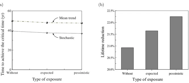
Figure 8a shows the influence of the weather model on the critical times for the different global warming scenarios and the continental environment. The following cases of weather modeling are compared: (1) only the mean trend is considered (Eq. 16); and (2) a stochastic variation is added (Eq. 17). For all the three scenarios, it is noted from Figure 8a that accounting for the randomness associated to weather reduces the critical times. By comparing both results (stochastic and mean trend) it is observed that this reduction is about 20% for all scenarios (see Figure 8b). This difference is explained by the presence of extreme values of temperature and humidity for the stochastic model that influences the chloride penetration process. Since these extreme values have been observed during real exposure conditions, these results justify the consideration of the randomness inherent to the phenomenon for a better lifetime assessment. It can be also noticed that the larger lifetime reductions correspond to the expected and pessimistic scenarios (Figure 8b). Although the difference is not important (from 20.9 to 22.3%), this behavior is due principally to the increase of temperatures and humidities induced by global warming that reduces the times to corrosion initiation.

The effect of global warming on the probability of corrosion initiation is presented in Figure 9. The curves plotted in this Figure correspond to the oceanic environment and all the considered locations. The overall behavior indicates that global warming increases the probability of corrosion initiation, particularly, for the pessimistic scenario. This increase is explained by the acceleration of the chloride flow induced by global warming which rises temperature and humidity as well as the length of the hot and wet periods. It can also be noted that the lifetime reduction induced by global warming is more significant for structures located far from the sea. Since the corrosion initiation time is shorter for higher surface chloride concentrations, the effect of global warming is less appreciable in this case. This means that in structures nearby the sea the process is completely dominated by high chloride concentrations at the surface and rarely influenced by climatic changes.

Figure 10a presents the critical times for all the considered environments and distances from the sea. It is observed that the shorter critical times correspond to the marine environments close to the sea. The difference between critical times for scenarios without and with global warming increases when the distance to the sea is more important. These results confirm that structures far from the ocean are more susceptible to be affected by global warming in terms of reduction of critical time. For instance global warming can reduce the critical times from 6 to 14 years for structures located at 3 km away from the seashore while this reduction is only from 1 to 3 years for d < 0.1 km. By comparing both marine environments, it can be also noted that the impact of global warming is most important for oceanic environments where the chloride ingress process is more sensitive to climatic changes.

Another way to analyze the results consists in computing the percentage of lifetime reduction taking as reference the case without global warming (Figure 10b). From these results it is observed that global warming induces lifetime reductions from 2 to 12% for the expected scenario and from 4 to 18% for the

pessimistic scenario. By comparing the average lifetime reduction for all the environments, the larger

influence corresponds to the oceanic environment (10.4%) followed by tropical environment (6.1%) and finally the continental environment (5.3%). These results justify the implementation of countermeasures directed to: (1) reduce and/or mitigate the action of global warming on weather and (2) minimize the impact of climate change on RC structures. These countermeasures should be adopted in function of specific features of the structure as the type of environment and the location.

6. Summary and conclusions

This paper presents a stochastic approach to study the influence of weather and global warming on chloride ingress into RC. The assessment of chloride ingress was carried out by using a comprehensive model that accounts mainly for the effects of convection, chloride binding, decrease of chloride diffusivity by concrete aging, temperature and humidity. The governing equations of the problem were solved by coupling finite element and finite difference methods. Since climate can influence the kinematics of chloride penetration, a model of weather that includes seasonal variation and global warming was also proposed in this paper. Finally the whole model is coupled with stochastic processes and probabilistic methods to account for the randomness involved in the process.

The proposed methodology is illustrated on the study of the impact of weather on corrosion initiation for various chloride-contaminated environments –i.e., continental, oceanic and tropical. The features of these environments depend on both latitude of the site and closeness to the sea. It was observed that the highest probabilities of corrosion initiation correspond to marine environments, in particular, for the tropical environment. These results are explained by the facts that (1) structures placed in marine environments are exposed to chlorides all the time and (2) higher temperatures and humidities accelerate the penetration of chloride ions into the concrete matrix. The probability of corrosion initiation increases for structures close to the sea. This effect is more appreciable for the tropical environment because larger values of temperature and humidity reduce the time to corrosion initiation. The probability of corrosion initiation is also influenced by global warming. The overall behavior indicates that the lifetime reduction induced by global warming is more significant for structures located in chloride-contaminated environments far from the sea. The results also indicate that the climate change effect is higher for structures located in oceanic environments and leads to lifetime reductions ranging from 2 to 18%. These results stress the importance of including a comprehensive model of chloride ingress and justify the implementation of countermeasures directed to (1) reduce and/or mitigate the action of global warming on weather and (2) minimize the impact of climate change on RC structures.

Acknowledgments

The authors acknowledge financial support of the project ’Maintenance and repair of concrete coastal structures: risk-based optimization’ (MAREO Project).

References

[1] Husni R. et al. Acciones sobre las estructuras de hormig´on. Red Rehabilitar CYTED, Guarulhos; 2003. p 39–108. (In Spanish)

[2] Bhide S. Material usage and condition of existing bridges in the U.S. Technical Report SR342, Portland Cement Associa-tion, Skokie, Ill, 1999.

[3] Tuutti K. Corrosion of steel in concrete. Swedish Cement and Concrete Institute, 1982.

[4] Saetta A, Scotta R, Vitaliani R. Analysis of chloride diffusion into partially saturated concrete. ACI Materials Journal 1993;90(5):441–51.

[5] Mart´ın-P´erez B, Pantazopoulou SJ, Thomas MDA. Numerical solution of mass transport equations in concrete structures. Computers and Structures 2001;79:1251–64.

[6] Bastidas-Arteaga E, Chateauneuf A, S´anchez-Silva M, Bressolette Ph, Schoefs F. A comprehensive probabilistic model of chloride ingress in unsaturated concrete. Submitted to Probabilistic Engineering Mechanics 2009.

[7] Houghton J. Global warming. Reports on Progress in Physics 2005;68:1343–403.

[8] Bastidas-Arteaga E, S´anchez-Silva M, Chateauneuf A, Ribas Silva M. Coupled reliability model of biodeterioration, chloride ingress and cracking for reinforced concrete structures. Structural Safety 2008;30:110–29.

[9] Bastidas-Arteaga E, Bressolette Ph, Chateauneuf A, S´anchez-Silva M. Probabilistic lifetime assessment of RC structures under coupled corrosion-fatigue processes. Structural Safety 2009 31:84–96.

[10] Kong JS, Ababneh AN, Frangopol DM, Xi Y. Reliability analysis of chloride penetration in saturated concrete. Probabilistic Engineering Mechanics 2002;17:305–15.

[11] Val DV, Trapper PA. Probabilistic evaluation of initiation time of chloride-induced corrosion. Reliability Engineering and System Safety 2008;93:364–72.

[12] Nilsson L-O, Massat M, Tang L. The effect of non-linear chloride binding on the prediction of chloride penetration into concrete structure. In: Malhotra V, editor. Durability of Concrete, ACI SP–145. Detroit, USA 1994. p 469–86.

[13] Tang L, Nilsson LO. Chloride binding capacity and binding isotherms of OPC pastes and mortars. Cement and Concrete Research 1993;23:247–53.

[14] Glass G, Buenfeld N. The influence of the chloride binding on the chloride induced corrosion risk in reinforced concrete. Corrosion Science 2000;42:329–44.

[15] Brunauer S, Skalny J, Bodor E. Adsorption in nonporous solids. Journal of Colloid Interface Science 1969;30:546–52. [16] Xi Y, Baˇzant Z, Jennings H. Moisture diffusion in cementitious materials – adsorption isotherms. Advanced Cement Based

Materials 1994;1:248–57.

[17] Neville A. Properties of Concrete (3rd ed.). Longman Scientific & Technical; 1981.

[18] Akita H, Fujiwara T, Ozaka Y. A practical procedure for the analysis of moisture transfer within concrete due to drying. Magazine of Concrete Research 1997;49:129–37.

[19] Khan A, Cook W, Mitchell D. Thermal properties and transient thermal analysis of structural members during hydration. ACI Materials Journal 1998;95:293–303.

[20] IPCC. Climate change 2007: The physical science basis. contribution of working group I to the fourth assessment report of the intergovernmental panel on climate change. Technical report, Intergovernmental Panel on Climate Change; 2007. [21] Ghanem RG, Spanos PD. Stochastic Finite Elements: A Spectral Approach. Springer, New York, USA; 1991.

[22] McGee R. Modelling of durability performance of Tasmanian bridges. In: Melchers RE and Stewart MG, editors. Appli-cations of statistics and probability in civil engineering,, Rotterdam: Balkema; 2000. p 297–306.

[23] Vu KAT, Stewart MG. Structural reliability of concrete bridges including improved chloride-induced corrosion. Structural Safety 2000;22:313–33.

[24] Duracrete. Statistical quantification of the variables in the limit state functions. Technical report, The European Union -Brite EuRam III - Contract BRPR-CT95-0132 - Project BE95-1347/R9, 2000.

[25] Page C, Short N, Tarras AE. Diffusion of chloride ions in hardened cement pastes. Cement and Concrete Research 1981;11:395–406.

[26] Val DV. Service-life performance of RC structures made with supplementary cementitious materials in chloride-contaminated environments. In: Proceedings of the international RILEM-JCI seminar on concrete durability and service life planning. Israel:Ein-Bokek;2006. p 363–73.

[27] Baˇzant Z, Najjar L. Drying of concrete as a nonlinear diffusion problem. Cement and Concrete Research 1971;1:461–73. [28] Baˇzant Z, Najjar L. Nonlinear water diffusion in nonsaturated concrete. Materials and Structures 1972;5:3–20.

Appendix A. Correction expressions for the diffusion coefficients Chloride diffusion coefficient

The expression to account for the temperature effect is given by [4]:

f1(T ) = exp  Uc R ✓ 1 Tref − 1 T ◆0 (24)

where Uc is the activation energy of the chloride diffusion which varies between 32 and 44.6 kJ/mol [25],

R is the gas constant (R = 8.314 J/(mol o_{K)), T}

ref is the reference temperature at which the reference

diffusion coefficient, Dc,ref, has been evaluated (Tref = 276 oK) and T is the actual absolute temperature

in the concrete ino_{K. The decrease of the diffusivity of concrete in time is evaluated from:}

f2(t) =✓ tref

t

◆m

(25)

where tref is the time of exposure at which Dc,ref has been evaluated (tref = 28 days), t is the actual time

of exposure in days and m is the age reduction factor varying between 0 − 1 [26]. Finally the influence of humidity is estimated from the expression:

f3(h) = " 1 + (1 − h) 4 (1 − hc)4 #−1 (26)

where hc is the humidity at which Dc drops halfway between its maximum and minimum values (i.e.,

hc = 0.75 [27]) and h is the actual pore relative humidity.

Humidity diffusion coefficient

g1(h) takes into consideration the dependence on the pore relative humidity of the concrete:

g1(h) = α0+

1 − α0

1 + [(1 − h)/(1 − hc)]n

(27)

where α0is a parameter that represents the ratio of Dh,min/Dh,max, hcis the value of pore relative humidity

at which Dhdrops halfway between its maximum and minimum values (hc= 0.75) and n is a parameter that

characterizes the spread of the drop in Dh. According to [27, 28], α0 and n fluctuate between [0.025 − 0.1]

and [6 − 16], respectively. g2(T ) accounts for the influence of the temperature on Dh:

g2(T ) = exp  U R ✓ 1 Tref − 1 T ◆0 (28) where U is the activation energy of the moisture diffusion process which oscillates between 22.5 and 39

kJ/mol and Tref is the reference temperature at which Dh,ref was measured (Tref = 276 ◦K). The last

relationship, g3(te), considers the dependency on the hydration period:

g3(te) = 0.3 +

r 13 te

List of Tables

Table 1. Correspondence between Eq. 1 and the governing differential equations.

Table 2. Parameters used to simulate global warming.

Table 3. Description of the studied environments.

Table 4. Probabilistic models of the random variables.

List of Figures

Figure 1. Algorithm for estimating the temperature, humidity and chloride profiles.

Figure 2. Mean of the weather model.

Figure 3. Example of the temperature model including global warming.

Figure 4. Time-variant and stochastic modeling of temperature.

Figure 5. (a) Stochastic surface chloride concentrations. (b) Mean of the concentration of de-icing salts.

Figure 6. (a) Problem description. (b) Effect of type of exposure.

Figure 7. Influence of the distance to the sea.

Figure 8. Comparison between weather models: (a) time to achieve the 95% of pcorr, (b) lifetime reduction.

Figure 9. Effect of global warming for the oceanic environment.

Table 1: Correspondence between Eq. 1 and the governing differential equations. Physical problem ψ ζ J J0 _q0s ψ Chloride ingress Cf c 1 D⇤c − ! rCf c Cf cDh⇤ − ! rh qs h Moisture diffusion h ∂we/∂h Dh − ! rh 0 0 Heat transfer T ρccq λ − ! rT 0 0

Table 2: Parameters used to simulate global warming.

Scenario Characteristics ∆Ta ∆ha ∆Ra

Without climate change is neglected 0o

C 0 0

Expected use of alternative and fossil sources of energy, birthrates follow

the current patterns and there is no an extensive employ of clean technologies.

2.5o

C 0.05 -0.1

Pessimistic vast utilization of fossil sources of energy, appreciable growth of population and there are no politics to develop and extent the use of clean technologies.

6.5o

C 0.10 -0.2

Table 3: Description of the studied environments.

Climate Description Temperature Humidity µCenv

Tmin Tmax hmin hmax

Continental places located at middle latitudes far from the ocean (see Fig. 4).

-10o

C 20o

C 0.6 0.8 Eq. 21

Oceanic structures placed at middle latitudes close

to the ocean.

5o

C 25o

C 0.6 0.8 Eq. 20

Tropical sites emplaced at equatorial latitudes close

to the ocean.

20o

C 30o

C 0.7 0.9 Eq. 20

Table 4: Probabilistic models of the random variables.

Physical problem Variable Mean COV Distribution

Chloride ingress Dc,ref 3 ⇥ 10−11m

2 /s 0.20 log-normal Cth 0.5 wt% cement 0.20 normal ct 50 mm 0.25 normala Uc 41.8 kJ/mol 0.10 beta on [32;44.6] m 0.15 0.30 beta on [0;1]

Moisture diffusion Dh,ref 3 ⇥ 10−10m

2

/s 0.20 log-normal

α0 0.05 0.20 beta on [0.025;0.1]

n 11 0.10 beta on [6;16]

Heat transfer λ 2.5 W/(m◦_{C) 0.20 beta on [1.4;3.6]}

ρc 2400 kg/m

3

0.20 normal

cq 1000 J/(kg◦C) 0.10 beta on [840;1170]

!"#$#%&'()"*#$#)"+

'''''''',)-'!"!

''

.#-+$'#$/-%$#)"'

#

_{!0 " !}

_!#!

"/1$'#'

!

!!

%# !

2)"3/-4/"(/

!!!!!!!!!!!!

2)"3/-4/"(/

!!!!!!!!!!!!

5/+

")

,)-'!'6'!

5/+

")

!"#$#%&'7-),#&/'

),'(8&)-#*/+

&

(

!"#$#%&'7-),#&/'

),'89:#*#$5

&

,

!"#$#%&'7-),#&/'

),'$/:7/-%$9-/

&

-

.#"*'$8/'7-),#&/'

),'(8&)-#*/+'%$'!

&

(

.#"*'$8/'7-),#&/'

),'89:#*#$5'%$'!

&

,

.#"*'$8/'7-),#&/'

),'$/:7/-%$9-/'%$'!

&

-'

'6'()3/-'$8#(;"/++

! "#$ %&'()'% &" ' &(% '* "+ *(#,' !" ! "#$ %&'()'% &" ' -(. /''* "+ *(#,' !# 012",'$

$

Figure 2: Mean of the weather model.

! " # $% $$ "!!

&'()*+,-.

&

)(

1

)-23

4

-)

*+

56

.

!"#$%&#'''''''''()*(+#(,'''''''''*(--"."-#"+

/

/

Figure 3: Example of the temperature model including global warming.

! " # $ % & '"& '"! '& ! & "! "& #! #& $! ()*+,-.+/012 ( +* 3 +0 /4 5 0+ ,-67 2 !"#$%&'("')*+#$') ,*-./'0*".+($'1"2'*"-)

(a) (b) ! " # $ % & ! & "! "& #! '()*+,-*./01 2 3 /4 .5 *+ 5 6 78 /( 9 *+ 5 8 : 5 *: ;/ .; (8 : +, < = >) ?1 !"#$%$&' !()*+, !(-, !(./+01 ! " !"#$%&# # $ '$()&* % ! " '$()&+ ! "

'$()&#$&,&* '$( )*+

,

µ,

-#.

,

Figure 5: (a) Stochastic surface chloride concentrations. (b) Mean of the concentration of de-icing salts.

(a) (b)

!

! "! #! $! %! &! ! !'# !'% !'( !') " *+,-./0-1234 5 26 7 17 +8+ 90 .6 :. ; 6 22 6 3+ 6 < .+ < +9 +1 9+ 6 < !"#$%&'( )&*'+%& ,-=-!'"->, ,-?-"->, ,-@-$->,

Figure 7: Influence of the distance to the sea.

(a) (b)

Without0 expected pessimistic

20 40 60 Type of exposure Stochastic Mean trend T im e to a ch ie v e t h e c ri ti ca l t im e ( y r) !"#$%&# '()'*#'+ )',,"-",#"* ./0/1 ./021 .30/1 .3021 ..0/1 ..021 45)'6%76'()%,&8' 9 "7 '# "-'6 8' + & * #" % :

! "! #! $! %! &! ! !'# !'% !'( !') " *+,-./0-1234 5 26 7 17 +8+ 90 .6 :. ; 6 22 6 3+ 6 < .+ < +9 +1 9+ 6 < !"#!$%!& '(%)*+% &,=,!'",>, _&,?,",>, &,@,$,>, #!--(.(-%($

Figure 9: Effect of global warming for the oceanic environment.

(a) (b) ! "! #! $! %! &'()*+(,,,,,,,,,,,,,,,,,-./01(02,,,,,,,,,,,,,,,3044'5'4('1 6 '5 0,( *,7 1) '0 80 ,9 :; ,*< ,, !"#$ $ "#%&'%(%&)* #"()%'" &$#!'")* +,=,>,?5 +,@,A,?5 +,B,!C>,?5 D10E7F'*4,*<,GH*I7H,J7F5'EG !"#$%#&#$'( )*"+%,'( -,&'#%, ./ 0/ 1/ 2/ 3/ 4./ 40/ 41/ 42/ 43/ 0./ !"#$%&$' ($))*+*)&*% )5+&6"76&8+"9:*& ; %7 &$ %< &6 *& = : , $% " # '>4,?< '@A,?< 'B.C4,?< 'B.C4,?< '>4,?< '@A,?<