HAL Id: hal-03052150
https://hal.archives-ouvertes.fr/hal-03052150
Submitted on 10 Dec 2020
HAL is a multi-disciplinary open access
archive for the deposit and dissemination of
sci-entific research documents, whether they are
pub-lished or not. The documents may come from
teaching and research institutions in France or
abroad, or from public or private research centers.
L’archive ouverte pluridisciplinaire HAL, est
destinée au dépôt et à la diffusion de documents
scientifiques de niveau recherche, publiés ou non,
émanant des établissements d’enseignement et de
recherche français ou étrangers, des laboratoires
publics ou privés.
differential phase shift and path-integrated attenuation
at the X band frequency in an Alpine environment
Guy Delrieu, Anil Kumar Khanal, Nan Yu, Frédéric Cazenave, Brice
Boudevillain, Nicolas Gaussiat
To cite this version:
Guy Delrieu, Anil Kumar Khanal, Nan Yu, Frédéric Cazenave, Brice Boudevillain, et al.. Preliminary
investigation of the relationship between differential phase shift and path-integrated attenuation at
the X band frequency in an Alpine environment. Atmospheric Measurement Techniques, European
Geosciences Union, 2020, 13 (7), pp.3731 - 3749. �10.5194/amt-13-3731-2020�. �hal-03052150�
https://doi.org/10.5194/amt-13-3731-2020 © Author(s) 2020. This work is distributed under the Creative Commons Attribution 4.0 License.
Preliminary investigation of the relationship between differential
phase shift and path-integrated attenuation at the X band frequency
in an Alpine environment
Guy Delrieu1, Anil Kumar Khanal1, Nan Yu2, Frédéric Cazenave1, Brice Boudevillain1, and Nicolas Gaussiat2
1Institut des Géosciences de l’Environnement (IGE, UMR 5001, Université Grenoble Alpes, CNRS, IRD),
Grenoble, France
2Centre de Météorologie Radar, Direction des Systèmes d’Observation, Météo-France, Toulouse, France
Correspondence: Guy Delrieu (guy.delrieu@univ-grenoble-alpes.fr) Received: 18 December 2019 – Discussion started: 13 January 2020 Revised: 25 May 2020 – Accepted: 10 June 2020 – Published: 10 July 2020
Abstract. The RadAlp experiment aims at developing ad-vanced methods for rainfall and snowfall estimation using weather radar remote sensing techniques in high mountain regions for improved water resource assessment and hydro-logical risk mitigation. A unique observation system has been deployed since 2016 in the Grenoble region of France. It is composed of an X-band radar operated by Météo-France on top of the Moucherotte mountain (1901 m above sea level; hereinafter MOUC radar). In the Grenoble valley (220 m above sea level; hereinafter a.s.l.), we operate a research X-band radar called XPORT and in situ sensors (weather sta-tion, rain gauge and disdrometer). In this paper we present a methodology for studying the relationship between the dif-ferential phase shift due to propagation in precipitation (8dp)
and path-integrated attenuation (PIA) at X band. This rela-tionship is critical for quantitative precipitation estimation (QPE) based on polarimetry due to severe attenuation effects in rain at the considered frequency. Furthermore, this rela-tionship is still poorly documented in the melting layer (ML) due to the complexity of the hydrometeors’ distributions in terms of size, shape and density. The available observation system offers promising features to improve this understand-ing and to subsequently better process the radar observations in the ML. We use the mountain reference technique (MRT) for direct PIA estimations associated with the decrease in re-turns from mountain targets during precipitation events. The polarimetric PIA estimations are based on the regularization of the profiles of the total differential phase shift (9dp) from
which the profiles of the specific differential phase shift on
propagation (Kdp) are derived. This is followed by the
ap-plication of relationships between the specific attenuation (k) and the specific differential phase shift. Such k–Kdp
relation-ships are estimated for rain by using drop size distribution (DSD) measurements available at ground level. Two sets of precipitation events are considered in this preliminary study, namely (i) nine convective cases with high rain rates which allow us to study the φdp–PIA relationship in rain, and (ii) a
stratiform case with moderate rain rates, for which the melt-ing layer (ML) rose up from about 1000 up to 2500 m a.s.l., where we were able to perform a horizontal scanning of the ML with the MOUC radar and a detailed analysis of the φdp–
PIA relationship in the various layers of the ML. A common methodology was developed for the two configurations with some specific parameterizations. The various sources of er-ror affecting the two PIA estimators are discussed, namely the stability of the dry weather mountain reference targets, radome attenuation, noise of the total differential phase shift profiles, contamination due to the differential phase shift on backscatter and relevance of the k–Kdp relationship derived
from DSD measurements, etc. In the end, the rain case study indicates that the relationship between MRT-derived PIAs and polarimetry-derived PIAs presents an overall coherence but quite a considerable dispersion (explained variance of 0.77). Interestingly, the nonlinear k–Kdprelationship derived
from independent DSD measurements yields almost unbi-ased PIA estimates. For the stratiform case, clear signatures of the MRT-derived PIAs, the corresponding φdp value and
av-eraged PIA/φdpratio, a proxy for the slope of a linear k–Kdp
relationship in the ML, peaks at the level of the copolar corre-lation coefficient (ρhv) peak, just below the reflectivity peak,
with a value of about 0.42 dB per degree. Its value in rain below the ML is 0.33 dB per degree, which is in rather good agreement with the slope of the linear k–Kdprelationship
de-rived from DSD measurements at ground level. The PIA/φdp
ratio remains quite high in the upper part of the ML, between 0.32 and 0.38 dB per degree, before tending towards 0 above the ML.
1 Introduction
Estimation of atmospheric precipitation (solid/liquid) is im-portant in a high mountain region such as the Alps for the assessment and management of water and snow resources for drinking water, hydropower production, agriculture and tourism characterized by high seasonal variability. One of the most critical applications concerns the prediction of natural hazards associated with intense precipitation and melting of snowpacks, i.e., inundations, floods, flash floods and grav-itational movements, which requires a high-resolution ob-servation, namely spatial resolution ≤ 1 km2 and temporal resolution ≤ 1 h. While this can hardly be achieved over ex-tended areas with traditional in situ rain gauge networks, the use of radar remote sensing has a high potential that needs to be exploited but also a number of limitations that need to be surpassed. Quantitative precipitation estimation (QPE) with radar remote sensing in a complex terrain such as the Alps is made challenging by the topography and the space– time structure and the dynamics of precipitation systems. Radar coverage of the mountain regions brings the follow-ing dilemma. On the one hand, installfollow-ing radar at the top of a mountain allows for a 360◦panoramic view and therefore the ability to detect precipitation systems over a long range at the regional scale. This is particularly relevant for localized and heavy convective systems in warm seasons. But the precipi-tation is likely to undergo a significant change between de-tection and arrival at ground level, including a phase change when the 0◦C isotherm is located at the level of or lower than the radar beam altitude. Such situations are likely to be frequent during cold periods, with a strong impact on QPE quality at ground level. On the other hand, installing a radar at the bottom of the valley provides high-resolution and qual-ity data required for vulnerable and densely populated Alpine valleys, but the QPEs are limited in the latter due to beam blockage by surrounding mountains.
In Europe, MeteoSwiss has the longest-standing expe-rience in operating radars in mountainous regions. The Swiss C-band radar network in the Alps (Joss and Lee, 1995; Germann et al., 2006) is one of the highest in the world and is coping with the associated altitude dilemma by using a large number of plan-position indicator (PPI)
scans (including negative elevation ones) aimed at deter-mining high-resolution vertical profiles of reflectivity. So-phisticated radar–rain gauge merging techniques and echo-tracking techniques, as well as numerical prediction models outputs (Sideris et al., 2014; Foresti et al., 2018) are im-plemented to better understand and quantify the complex-ity of precipitation distribution in such a rugged environ-ment. More recently, Météo-France has chosen to comple-ment the coverage of its operational radar network of Appli-cation Radar à la Météorologie Infra-Synoptique (ARAMIS) in the Alps by means of X-band polarimetric radars. A first set of three radars was installed in the southern Alps within the Risques Hydrométéorologiques en Territoires de Mon-tagnes et Méditerranéens (RHyTMME) project in the period 2008–2013 at Montagne de Maurel (1770 m above sea level; hereinafter a.s.l.), Mont Colombis (1740 m a.s.l.) and Vars Mayt (2400 m a.s.l.; Westrelin et al., 2012). This effort was continued in 2014–2015 with the installation of an additional X-band radar system (hereinafter MOUC radar) on top of the Moucherotte mountain (1920 m) that dominates the valley of Grenoble, the biggest city in the French Alps with about 500 000 inhabitants. The choice of the X-band frequency is challenging due to its sensitivity to attenuation (e.g., Delrieu et al., 2000). In the past, the Institute of Environmental Geo-sciences (IGE) radar team has proposed the so-called moun-tain reference technique (MRT; Delrieu et al., 1997; Serrar et al., 2000; Bouilloud et al., 2009) to take advantage of this drawback for both correcting the gate-to-gate attenuation and performing a self-calibration of the radar. The idea was to es-timate the path-integrated attenuations (PIAs) in some spe-cific directions from the decrease in mountain returns during rainy periods. Such PIA estimates were then used as con-straints for backward or forward attenuation correction algo-rithms (Marzoug and Amayenc, 1994) with optimization of an effective radar calibration error, given a drop size distribu-tion (DSD) parameterizadistribu-tion. The development of polarimet-ric radar techniques (e.g., Bringi and Chandrasekar, 2001; Ryzhkov et al., 2005) has allowed a scientific breakthrough for quantitative precipitation estimation (QPE) at X band by exploiting the relationship which exists between the spe-cific differential phase shift on propagation (Kdp, in◦km−1)
and the specific attenuation k (dB km−1). As with the MRT, the differential propagation phase 8dp(r2) − 8dp(r1)over a
given path (r1, r2)can be used to estimate PIA(r1, r2), which
can constrain a backward attenuation correction algorithm and allow a self-calibration of the radar and/or an adjustment of the DSD parameterization (Testud et al., 2000; Ryzhkov et al., 2014). Two major advantages of the polarimetric tech-nique over the MRT can be formulated, namely (1) the avail-ability of PIA constraints for any direction with significant precipitation and (2) the subsequent possibility of using a backward attenuation correction algorithm, which is known to be stable, while the forward formulation is inherently un-stable. Accounting for their respective potential in different rain regimes (moderate to heavy), some combined algorithms
making use of various polarimetric observables (reflectivity, differential reflectivity and specific differential phase shift on propagation) have also been proposed for the X-band fre-quency (e.g., Matrosov and Clark, 2002; Matrosov et al., 2005; Koffi et al., 2014). Although the polarimetric QPE methodology is now quite well established and validated for rainy precipitation (Matrosov et al., 2005; Anagnostou et al., 2004; Diss et al., 2009), Yu et al. (2018) have shown, in their first performance assessment of the RHyTMME radar net-work, the limitations associated with the use of polarimetric X-band radars in mountainous regions. They have pointed out (i) the need to better understand and quantify attenua-tion effects in the melting layer (ML), (ii) the importance of nonuniform beam filling (NUBF) effects at medium-to-long ranges in such a high-mountain context, and (iii) the stronger impact of radome attenuation at X band compared to S or C band. Yu et al. (2018) also had a first attempt at studying the relationship between the specific differential phase shift on propagation and the specific attenuation in the melting later by using the collocated measurements of two X-band radars, one situated well below and the other one situated well above the 0◦C isotherm, and by considering the attenuation uni-form within the ML.
Since 2016, we have had the opportunity to operate a research X-band polarimetric radar system (hereinafter XPORT radar) at IGE at the bottom of the Grenoble val-ley. This unique facility, consisting of two radar systems 11 km apart and operating on an altitudinal gradient of about 1700 m, should enable us to make progress on how to deal with the altitude dilemma and the potential/issues associated with the choice of the X-band operating frequency. Follow-ing a first article based on the RadAlp experiment about the characterization of the melting layer (Khanal et al., 2019), we concentrate hereinafter on the relationship between total dif-ferential phase shift (φdp) derived from polarimetry and PIAs
derived from the MRT. In Sect. 2, we present the observation system available and contrast rainy events considered in this study as follows: (i) a set of nine convective events with high rain rates, for which the melting layer was well above the de-tection domain of the XPORT radar, allows us to study the φdp−PIA relationship in rain; and (ii) a stratiform case with
moderate rain rates, for which the melting layer rose up from about 1000 to 2500 m a.s.l., allows us to perform a horizontal scanning of the ML with the MOUC radar and a preliminary analysis of the φdp−PIA relationship in the various layers of
the ML. We present and illustrate, in Sect. 3, the methodol-ogy used for the PIA and φdpestimation. We also investigate
the relationship between the specific differential phase shift on propagation (Kdp) and the specific attenuation (k) thanks
to drop size distribution (DSD) measurements collected in the Grenoble valley during the two sets of events. The re-sults concerning the φdp–PIA relationship in rain and in the
ML are presented and discussed in Sect. 4, while conclusions and perspectives are drawn in Sect. 5.
2 Observation system and datasets 2.1 Observation system
Grenoble is a y-shaped alluvial valley in the French Alps, with a mean altitude of about 220 m a.s.l. and surrounded by three mountain ranges, namely the Chartreuse (culminat-ing at 2083 m a.s.l.) to the north, the Belledonne (2977 m) to the southeast and the Vercors (2307 m) to the west. Fig-ure 1 shows the topography of the area and the positions of the Météo-France radar system on top of the Moucherotte mountain and the IGE experimental site at the bottom of the valley.
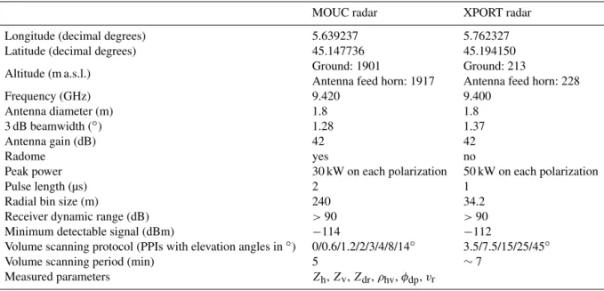
Among other devices, the IGE experimental site includes the following: (i) the IGE XPORT research radar (Koffi et al., 2014; see Table 1 for the list of its main parameters); (ii) one Micro Rain Radar (MRR; not used in the current study); (iii) one meteorological station including pressure, temperature, humidity, wind probes and several rain gauges; and (iv) one Parsivel2disdrometer. The characteristics of the MOUC radar are listed in Table 1. XPORT radar was built in the laboratory in the 2000s. It was operated during more than 10 years in western Africa within the African Monsoon Multidisciplinary Analysis (AMMA) and Megha-Tropiques calibration/validation campaigns. Since its return to France in 2016, a maintenance and updating program has been un-derway to improve its functionalities, notably with respect to the real-time data processing and the antenna control pro-gram. One noticeable feature of XPORT radar is the range bin size of 34.2 m (which actually corresponds to an over-sampling since, for a pulse width of 1 µs, the theoretical bin size is 150 m), which is an interesting figure for the close-range and volumetric measurements considered in this study. Note that while the MOUC radar is operated 24 h per day and its data are integrated in the Météo-France mosaic radar products, the XPORT radar is operated with alerts only on for significant precipitation events.
2.2 Dataset
Table 2 shows the main characteristics of the nine convec-tive events considered for the study of the φdp–PIA
relation-ship in rain, by using the XPORT radar data. A stratiform event, which occurred on 3–4 January 2018, is also consid-ered for a preliminary study of the φdp–PIA relationship in
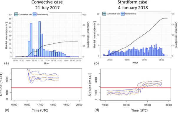
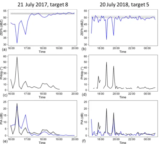
the ML, with both the MOUC and the XPORT radar data. Figure 2 presents a time series of one of the most intense convective event (21 July 2017) and the stratiform event. In both cases, the total rain amount observed at the IGE site was about 35 mm, but in 3 h, with two peak rain rates of about 40 mm h−1for the 21 July 2017 convective event, while the 3–4 January 2018 stratiform event lasted more than 12 h with an average rain rate of about 3 mm h−1. The two events also differ in their vertical structure. The bottom graphs of Fig. 2 display the time series of the altitudes of the tops, peaks
Figure 1. The topographical map of Grenoble is shown along with the positions of two radar systems. A vertical cross section along the line joining the two radar sites is shown in the insert at the bottom right of the figure.
Table 1. Characteristics of the XPORT and MOUC radar systems.
MOUC radar XPORT radar Longitude (decimal degrees) 5.639237 5.762327 Latitude (decimal degrees) 45.147736 45.194150 Altitude (m a.s.l.) Ground: 1901 Ground: 213
Antenna feed horn: 1917 Antenna feed horn: 228
Frequency (GHz) 9.420 9.400
Antenna diameter (m) 1.8 1.8
3 dB beamwidth (◦) 1.28 1.37
Antenna gain (dB) 42 42
Radome yes no
Peak power 30 kW on each polarization 50 kW on each polarization
Pulse length (µs) 2 1
Radial bin size (m) 240 34.2
Receiver dynamic range (dB) >90 >90 Minimum detectable signal (dBm) −114 −112
Volume scanning protocol (PPIs with elevation angles in◦) 0/0.6/1.2/2/3/4/8/14◦ 3.5/7.5/15/25/45◦ Volume scanning period (min) 5 ∼7
Measured parameters Zh, Zv, Zdr, ρhv, φdp, vr
and bottoms of the horizontal reflectivity (Zh) and copolar
correlation coefficient (ρhv) signatures of the ML, obtained
with the automatic detection algorithm described in Khanal et al. (2019). The quasi-vertical profiles (QVP; Ryzhkov et al., 2016) derived from the XPORT 25◦PPIs are considered
in the ML detection. For the convective case, the ML extends from 3000 to 4000 m a.s.l. and more, i.e., well above the
alti-tudes of the two radars. Table 2 indicates that this is also the case for the other convective events – at least for the XPORT radar. For the stratiform event, the ML extends between 800 and 1500 m a.s.l. during the first part of the event (between 3 January, 20:00 UTC, and 4 January, 01:30 UTC) and then rises in about 2 h to stabilize at an altitude range of about
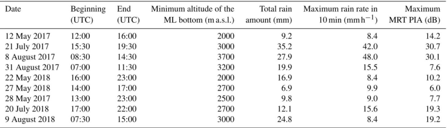
Table 2. Some characteristics of the nine convective events considered in the study of the φdp–PIA relationship in rain. The ML detection was performed with the 25◦elevation angle measurements of the XPORT radar using the algorithm described in Khanal et al. (2019). The total rain amount and the maximum rain rate are recorded at the weather station available at the XPORT radar site at IGE. The maximum PIA is derived from the MRT by considering the 7.5◦elevation data of the XPORT radar.
Date Beginning End Minimum altitude of the Total rain Maximum rain rate in Maximum (UTC) (UTC) ML bottom (m a.s.l.) amount (mm) 10 min (mm h−1) MRT PIA (dB) 12 May 2017 12:00 16:00 2000 9.2 8.4 14.2 21 July 2017 15:30 19:30 3000 35.2 42.0 30.7 8 August 2017 08:30 14:30 3700 27.9 48.0 30.1 31 August 2017 07:00 11:30 3200 19.9 15.5 7.6 22 May 2018 16:00 23:00 2000 16.9 8.4 10.2 27 May 2018 14:00 17:00 2700 6.9 9.9 6.0 28 May 2017 13:00 23:00 2500 9.8 9.0 7.7 20 July 2018 17:00 22:00 2700 12.1 15.6 19.3 9 August 2018 07:30 15:00 3000 24.8 8.4 19.2
2200–2800 m a.s.l. after 04:00 UTC, passing progressively at the level of the MOUC radar in the meantime.
As an additional illustration of the dataset, Fig. 3 gives two examples of XPORT PPIs at 7.5◦elevation angle for
mod-erate (left) and intense (right) rain during the 21 July 2017 event. As a clear feature, one can see that, for this eleva-tion angle, the radar beam is fully blocked by the Chartreuse mountain range in the northern sector. Also visible in the northeastern sector and, to a lesser extent, in the southwest-ern sector are partial beam blockages associated with tall trees in the vicinity of the XPORT radar on the Greno-ble campus. This figure is also intended to draw the atten-tion of the reader to the decrease in the Chamrousse and Moucherotte mountains returns (within red circles) during the intense rain time step, compared to their values in mod-erate rain, as a first illustration of the MRT principle.
3 Methodology
Our aim is to study the relationship between two radar ob-servables of propagation effects at X band, namely path-integrated attenuation and differential propagation phase due to precipitation occurring along the radar path. We describe, in the following two subsections, the estimation methods that were implemented. In Sect. 3.3, we complement the method-ology description with the presentation of DSD-derived k– Kdprelationships.
3.1 Path-integrated attenuation estimation
Let us express the PIAs (in dB) at a given range r (km) as follows: PIA (r) = PIA (r0) +2 r Z r0 k (s)ds, (1)
where k(s) (dB km−1) is the specific attenuation due to rain at range s (km). r0is the range where the measurements start
to become exploitable, i.e., the range where measurements are free of ground clutter associated with side lobe effects. The term PIA (r0) represents the so-called on-site
attenua-tion resulting from radome attenuaattenua-tion and range attenuaattenua-tion at range closer than r0. Note that PIAs can be obtained from
Eq. (1) for both the horizontal and the vertical polarizations. In the present article, we will restrict ourselves to the hori-zontal polarization, as the study of differential attenuation is a possible topic for a future study. Delrieu et al. (1999) have proposed an assessment of the quality of PIA estimates from mountain returns by implementing a receiving antenna in the Belledonne mountain range in conjunction with an X-band radar operated on the Grenoble campus. They found good agreement between the two PIA estimates for PIAs exceed-ing the natural variability of the mountain reference target during dry weather. They recommended using strong moun-tain returns (greater than, e.g., 50 dBZ during dry weather) so as to minimize the impact of precipitation falling over the reference target itself. They also point out that this approach is not able to separate the effects of on-site and range attenu-ation. They verified, however, by implementing the receiving antenna close to the radar (at a range of about 200 m), that the on-site attenuation was negligible for a radomeless radar, which is the case for the XPORT radar but not for the MOUC radar. Another interesting feature of the MRT PIA estimator is its independence with respect to eventual radar calibration errors.
Figure 2. Description of two rain events considered in the present study: (a, c) convective case of 21 July 2017 and (b, d) stratiform case of 4 January 2018. (a, b) Rain rate and cumulative rainfall time series observed at the IGE site and (c, d) results of the ML detection algorithm based on XPORT 25◦PPI data. The horizontal red line indicates the altitude of the MOUC radar (see text for details).
Figure 3. Examples of XPORT 7.5◦PPIs of raw reflectivity (not corrected for attenuation) taken for two time steps during the 21 July 2017 convective event. The crosses indicate the location of the two radars and the black/white (5/10 km) range markers correspond to the XPORT and the MOUC radar, respectively. The red circles highlight the mountain returns associated with the Chamrousse (southeast) and the Moucherotte (southwest) mountains in between the 10–15 km range.
In the current study, we used the following procedure to determine the mountain reference targets for the XPORT radar.
A large series of raw reflectivity data, observed during widespread rainfall with no ML contamination, was accu-mulated and averaged in order to characterize the detection domain of the XPORT radar at the 7.5◦elevation angle. This allowed us to determine the mountain returns, the full beam blockages due to mountains, the partial beam blockages due to tall trees and spurious detections due to side lobes in the vicinity of the radar. A manual selection of the mountain ref-erence targets was then performed based on the map of the apparent reflectivity above 45 dBZ. The targets, made up of mountain returns from successive radials (up to 9) with a lim-ited range extent (less than 2.0 km), are described in Table 3. Based on the radar equation and the receiver characteristics, care was taken to discard targets eventually subject to satura-tion at close range. The selected targets are located at a mean range between 4.1 and 17.1 km and have sizes between 0.06 and 0.94 km2. For each rain event, dry weather data before and/or after the event were used to characterize the mean tar-get reflectivity and its time variability. Note that the mean reflectivity for each target and each time step was computed as the average of the dBZ values of each radial gate com-prising the target. This is justified by the fact that we aim at estimating PIAs in dB. Table 3 lists the mean, standard devi-ation and 10 % and 90 % quantiles of the time series of the dry weather apparent reflectivity of the reference targets for the first and last event of the considered series. One can no-tice the good stability of the mean reflectivity values between the two events, which is an indication of both the radar cal-ibration stability during the period and the moderate impact of the mountain surface conditions already evidenced in pre-vious studies (Delrieu et al., 1999; Serrar et al., 2000). The standard deviations of the reflectivity time series range be-tween 0.2 and 0.9 dBZ, and the mean 10 %–90 % interquan-tile range is equal to 1.03 dBZ.
Due to limited data availability, a simpler approach was implemented for the selection of the MOUC mountain ref-erence targets. Here again, the raw reflectivity data were ac-cumulated and averaged, but only over the period of 3 Jan-uary 2018, 19:00–23:55 UTC, preceding the rise of the ML at the level of the MOUC radar. It was snowing during this period at the MOUC radar site. So, we are implicitly mak-ing the assumption of negligible attenuation durmak-ing snowfall (supported by the literature; e.g., Matrosov et al., 2009) in the considered case study. Table 4 displays the geometrical char-acteristics of the targets, as well as the mean, standard devia-tion and 10 % and 90 % quantiles of their apparent reflectiv-ity time series. Targets are located at greater distances than those of the XPORT radar, i.e., between 19.9 and 44.9 km. In spite of having larger sizes (between 0.7 and 4.0 km2), this range effect probably explains why their standard deviations are higher, namely between 0.75 and 1.44 dBZ. The 10 %–
90 % interquantile ranges are subsequently higher as well, with a mean value of 2.6 dBZ.
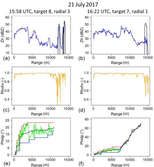
The top graphs of Fig. 4 give two examples of appar-ent reflectivity profiles for a radial of a given target during the 21 July 2017 rain event. The example on the left-hand side corresponds to a moderate PIA (5.4 dB, when consid-ering all the gates of the radials comprising the target) and the right-hand side example corresponds to one of the high-est PIA value observed (27.6 dB) in our dataset. We tried to limit, as far as possible, the radial extent of targets (less than 2000 m) and/or multipeaks targets, such as the one shown in the left-hand side example, in order to limit positive bias on MRT PIA estimates. The top graphs of Fig. 5 give two ex-amples of apparent reflectivity time series during the events of 21 July 2017 and 20 July 2018, together with the mean, 10 % and 90 % quantiles of the dry weather apparent reflec-tivity. For both cases, the XPORT data acquisition started a bit after the actual beginning of the storm. Therefore, the dry weather reference values were estimated with data collected after the event, i.e., between 19:00 and 22:00 UTC for the 21 July 2017 event and between 00:00 and 06:00 UTC on the day after for the 20 July 2018 event. For these convective events, one can note the erratic nature of the apparent reflec-tivity time series at the XPORT radar acquisition period used at that time (about 7 min). The MRT PIA estimates are sim-ply calculated as the difference between the mean values of the target apparent reflectivity during dry weather and at each time step of the rain event (blue lines in the bottom graphs of Fig. 5).
3.2 Differential propagation phase estimation
Let us express the total differential phase shift between copo-lar (HH and VV) received signals as follows:
ψdp(r) =2 r
Z
r0
Kdp(s)ds + δhv(r), (2)
where Kdp(s)is the specific differential phase shift on
prop-agation (◦km−1) related to precipitation at any range s be-tween r0and r, and δhv(r)is the differential phase shift on
backscatter (◦) at range r.
The quantity of interest, i.e., the differential propagation phase associated with precipitation along the path, is denoted as follows: φdp(r) =2 r Z r0 Kdp(s)ds = ψdp(r) − δhv(r). (3)
As with the on-site attenuation for the MRT, we have a problem here with the possible influence of the differential phase shift on backscatter δhv(r)that may introduce a
posi-tive bias on the estimation of the differential phase shift asso-ciated with precipitation along the path. In the literature (e.g.,
Table 3. Geometrical characteristics and apparent reflectivity statistics for the 16 mountain targets selected for the XPORT radar at an elevation angle of 7.5◦. The mean, standard deviation, and 10 % and 90 % quantiles of the apparent reflectivity time series are given for the first and last convective events in the considered period (see Table 2).
12 May 2017 9 August 2018
Target Mean Mean Number Size Mean Standard 10 % 90 % Mean Standard 10 % 90 %
azimuth range of gates (km2) reflectivity deviation quantile quantile reflectivity deviation quantile quantile
(◦) (km) (dBZ) (dBZ) (dBZ) (dBZ) (dBZ) (dBZ) (dBZ) (dBZ) 1 2.9 4.1 51 0.06 48.39 0.21 48.17 48.73 48.29 0.23 48.03 48.62 2 13.2 4.8 130 0.18 52.19 0.80 51.55 53.17 52.22 0.66 51.62 53.27 3 17.5 5.7 163 0.27 51.90 0.29 51.61 52.25 52.42 0.50 51.91 53.14 4 24.0 8.6 133 0.33 51.98 0.51 51.44 52.80 51.87 0.40 51.41 52.39 5 29.0 14.6 71 0.30 49.44 0.55 48.91 50.01 50.31 0.59 49.63 51.10 6 89.5 17.1 160 0.79 53.20 0.38 52.81 53.59 52.78 0.43 52.34 53.53 7 95.3 14.5 95 0.40 54.12 0.23 53.91 54.30 53.96 0.21 53.72 54.20 8 98.4 13.2 120 0.45 51.02 0.50 50.59 51.67 52.13 0.39 51.69 52.67 9 101.2 13.1 156 0.58 48.95 0.23 48.71 49.18 49.50 0.12 49.37 49.66 10 119.7 12.1 92 0.32 49.36 0.21 49.11 49.59 50.23 0.12 50.07 50.39 11 124.8 11.8 242 0.82 51.04 0.53 50.50 51.84 52.02 0.32 51.63 52.43 12 130.1 11.9 240 0.82 51.43 0.90 50.48 52.63 54.63 0.52 54.08 55.30 13 135.1 12.0 271 0.94 50.20 0.87 49.33 51.48 53.24 0.78 52.34 54.35 14 238.8 11.4 221 0.73 52.97 0.67 52.20 53.59 52.86 0.58 52.11 53.60 15 243.8 10.7 187 0.58 52.63 0.59 51.97 53.46 53.79 0.35 53.37 54.23 16 248.8 10.5 162 0.49 53.62 0.41 53.11 54.02 52.96 0.37 52.53 53.50
Table 4. Geometrical characteristics and apparent reflectivity statistics for the 13 mountain targets selected for the MOUC radar at an elevation angle of 0◦. The mean, standard deviation, and 10 % and 90 % quantiles of the apparent reflectivity time series are computed over the period of 3 January 2018 from 19:00 to 23:55 UTC, preceding the rising of the ML at the level of the MOUC radar.
3–4 January 2018
Target Mean azimuth Mean range Number Size Mean reflectivity Standard deviation 10 % quantile 90 % quantile (◦) (km) of gates (km2) (dBZ) (dBZ) (dBZ) (dBZ) 1 40.0 29.52 25 1.55 49.97 1.1 48.70 51.26 2 43.7 26.28 13 0.72 49.90 1.28 48.18 51.36 3 78.0 27.12 24 1.36 48.18 1.44 46.77 50.12 4 84.2 23.64 28 1.39 49.56 0.95 48.37 50.90 5 89.5 23.04 82 3.96 49.09 0.62 48.39 49.80 6 96.0 21.36 78 3.49 49.37 0.75 48.32 50.34 7 101.7 19.92 52 2.17 49.31 1.01 47.83 50.37 8 107.2 22.44 33 1.55 51.94 1.11 50.52 53.22 9 117.0 25.32 38 2.02 51.50 1.03 50.17 52.74 10 121.2 23.52 41 2.02 48.65 1.18 47.28 50.18 11 128.5 28.44 43 2.56 49.38 0.98 48.21 50.59 12 132.5 27.00 25 1.41 50.33 1.24 48.71 51.81 13 160.2 44.88 37 3.48 49.91 1.00 48.69 51.11
Otto and Russchenberg, 2011; Schneebeli and Berne, 2012) we find power law relationships between δhv and Zdr at X
band in rain, giving values for the differential phase shift on backscatter in the ranges of [0.6–1.0◦] and [2.1–3.5◦] for the differential reflectivity of 1 and 2 dB, respectively. Scattering simulations based on disdrometer data (Trömel et al., 2013) indicate that quite a large scatter may exist with respect to such power law models, and there is an important influence from the considered hydrometeor temperature. From
simu-lations based on radar data at various frequencies, the same authors quantify δhv(r)values as high as 4◦in the ML at X
band and mention that strong δhv(r) values may be
associ-ated with both large dry hailstones and wet hailstones, espe-cially at X band. Let us note that no hail was reported for the convective cases considered in the present study. Keep-ing the related orders of magnitude in mind, and the fact that significant δhv effects are associated with bumps in the ψdp
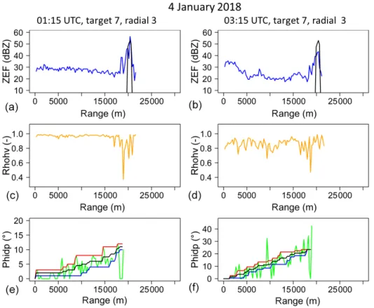
Figure 4. Two examples (right and left columns) of Zh, ρhv, and φdprange profiles of the XPORT radar (7.5◦PPI) during the 21 July 2017 convective event for one radial of a given mountain target. The raw horizontal reflectivity profiles (a, b) at the considered time steps (blue) are displayed together with the dry weather reference target value (black). The ρhvprofiles (c, d) are used to detect the rainy gates not affected by clutter at close range and in the region of the mountain target. Panels (e) and (f) display the raw ψdpprofiles (green), the upper (red) and lower (blue) envelope curves, and the regularized φdpprofiles (black).
profiles, hereafter we will carefully discuss the possibility of assuming δhvto be negligible, or not, with respect to φdp.
In this study, the following method was implemented for the processing of the ψdpprofiles and the subsequent
estima-tion of φdp values near the mountain targets for the XPORT
radar (rain case based on convective events).
We first determined so-called rainy range gates along the path by using the ρhv profiles. The raw ψdp(r)values, for
which ρhv(r) was less than 0.95 (empirical threshold with
limited impact in the [0.95–0.97] range), were set to miss-ing values. In addition, we defined the beginnmiss-ing of the rainy range by determining the first series of 10 successive gates (again, an empirical choice corresponding to a range extent of 342 m) overpassing this threshold. The r0value was set
to the minimum range value of this series. Similarly, we de-fined the end of the rainy range by determining the last
se-ries of 10 successive range gates overpassing this threshold close to the mountain target. A maximum rainy range, de-noted as rM, was defined as the maximum range value of this
series. It is noteworthy to mention that rain likely occurs in the ranges less than r0 and greater than rM and in the
in-termediate ranges for which the ψdp(r)values were set to
missing values. It is, however, critical to discard such gates that may be prone to clutter due to side lobes close to the radar or mountain returns close to the mountain target. Al-though the intermediate missing values will not impact the φdp estimation, we have to mention that both the initial and
final missing values may result in a negative bias on the PIA estimation based on φdp(rM).
In the current version of the procedure, every single radial was processed separately. First, an unfolding was applied by adding 360◦to negative ψdp(r)values. The system
differen-Figure 5. Two examples of time series of the apparent reflectivity of mountain returns for a given target (a, b), the corresponding 8dp estimates (c, d), and the resulting PIA estimates. The horizontal black lines in the top graphs represent the mean (solid line) and the 10 % and 90 % quantiles (broken lines) of the dry weather apparent reflectivity of the target. The three lines in (e) and (f) correspond to the MRT PIA estimates (blue) and to the polarimetry-derived PIA estimates by using the linear k–Kdprelationship (gray) and the nonlinear k–Kdp relationship (black) derived from DSD measurements at ground level.
tial phase shift was estimated as the median of the ψdp(r)
val-ues corresponding to the beginning of the rainy range. This value was subtracted from the raw ψdp(r)profiles, and
even-tual negative values were set to 0. Regarding the ψdp
mea-surement noise processing, we have implemented and im-proved a regularization procedure initially proposed by Yu and Gaussiat (2018). This procedure consists of defining an upper envelope curve, starting from r0, and a lower envelope
curve, starting from rM, by considering a maximum jump,
denoted as diffmax, authorized between two successive gates. The calculation was performed for a series of diffmax val-ues in the range of 0.5–10◦. The regularized ψ
dpprofiles
(in-creasing monotonous curves) were estimated by taking the average of the upper and lower envelope curves. Note that the values for the missing gates between r0and rMwere simply
interpolated with the adjacent values of the regularized pro-file. A mean absolute difference (MAD) criterion between the raw and regularized profiles over a series of 30 gates with nonmissing values near the mountain target (an empir-ical choice corresponding to a range extent of about 1 km) was used to determine the optimal diffmax value and the as-sociated profile. The optimal profile was finally selected if
the MAD criterion was less than 50 %, otherwise we con-sidered the polarimetry-derived PIAs to be missing for the considered radial. Finally, the φdp(rM)value for the target
was estimated as a weighted average of the φdp(rM)values
of all the nonmissing radials composing the target, with the weights being the number of reference gates of each radial. The bottom graphs of Fig. 4 present the raw and regularized profiles, and the envelope curves, for the examples already commented on above. For the right-side hand example cor-responding to one of the strongest PIAs (27.6 dB) observed, one can note that the noise of the raw ψdpprofile is low,
es-pecially in the range with the highest gradients between 7 and 13 km. There is no apparent bump on the raw profile that could signal a δhv contamination so that one might be
tempted to consider the regularized profile as a good estima-tor of the φdpprofile in that case. The left-hand side example,
corresponding to a moderate MRT-derived PIA of 5.4 dB, is more complex. As already noted, the mountain target itself is noisy with significant mountain return contamination before range rM, as evidenced by the ρhvprofile. In addition, one can
note a nonmonotonic behavior of the raw ψdpprofile, with a
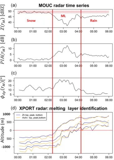
follow-Figure 6. Time series of (a) the apparent reflectivity values of a given mountain reference target together with the dry weather ref-erence (solid red horizontal lines for the mean) and the 10 % and 90 % quantiles (broken red lines), (b) the resulting PIA estimates (dB), and (c) the corresponding φdp(rM)values (◦) for the 0◦PPI of the MOUC radar during the 3–4 January 2018 stratiform rain event. (d) displays the results of the ML detection algorithm performed with the XPORT 25◦PPI data (see text for details).
ing an increase in the raw profile (with moderate noise) up to 22◦at a 4 km range. One might assume that there is a δhv
contamination in that case. Interestingly, the regularization procedure is shown to provide a good filtering of the bump, and here again we are tempted to consider the regularized profile as a good estimator of the φdp profile. The middle
graphs in Fig. 5 display the time series of the φdp(rM)
val-ues associated with the apparent reflectivity of the mountain returns discussed above. One can note good consistency in the two time series for the highest peaks, while discrepancies can be evidenced for the moderate and small values.
Basically, the same methodology was implemented for the MOUC radar case study, with some alterations to be de-scribed hereafter. Figure 6 provides the time series of the apparent reflectivity of a given mountain target, the
result-ing PIA estimates and the φdp(rM)estimates for the 0◦PPI
of the MOUC radar during the stratiform event of 3–4 Jan-uary 2018. The time period considered in the figure ranges from 00:00 to 06:00 UTC on 4 January 2018 in order to fo-cus on the rising of the ML between 02:00 and 04:00 UTC. The target is located at a distance of 19.9 km from the radar. The bottom graph of Fig. 6 displays the results of the ML detection algorithm (Khanal et al., 2019) in terms of the alti-tudes of the top, peak and bottom of the Zh(blue) and the ρhv
(orange) ML signatures. The altitude of the Zhtop inflexion
point is assumed to correspond to the 0◦C isotherm altitude, while the ρhv bottom inflexion point corresponds well with
the bottom of the ML according to Khanal et al. (2019). We therefore define the ML width as the altitude difference be-tween Zh top and ρhv bottom. Before 02:00 UTC, the ML
is well below the altitude of the MOUC radar. MOUC radar measurements at the 0◦ elevation angle are therefore made
in snow/ice precipitation during this period. Based on the ML detection results, the passage of the ML at the altitude of the MOUC radar begins at about 02:20 UTC and ends at 04:10 UTC. After this time, MOUC radar measurements are therefore made in rainfall.
As representative examples, Fig. 7 illustrates the range profiles taken by the MOUC radar during the snowfall (left) and the ML (right) periods. As expected, the ρhv profiles
are very different in the two cases, with ρhv values close to
1 in snow, indicating precipitation homogeneity while ρhv
presents a high variability in the ML. During the ML period, we therefore had to adapt the ρhv threshold used to detect
gates with precipitation. Based on the ρhvpeak statistics
pre-sented by Khanal et al. (2019), we have chosen a value of 0.8. As it can be seen in Fig. 7, such a threshold may prevent the detection of the mountain reference return itself. Subse-quently, we had to adapt the determination of ranges r0and
rMwith respect to the XPORT radar case, firstly, by
consid-ering two successive gates corresponding to a range extent of 480 m (instead of 10 gates corresponding to 342 m) and, secondly, by making sure that the calculated rM value was
less than the range of the first mountain reference gate. Re-garding the regularization of the ψdpprofiles (bottom graphs
of Fig. 7), it was found that the raw profiles were noisier compared to the XPORT case study. Well-structured bumps were not evidenced in the ML profiles, maybe as a result of the lower-range resolution of the MOUC radar, and the reg-ularization procedure was found to work satisfactorily. It re-mains, however, difficult to assume that there is no δhv
con-tamination during the ML period.
Coming back to Fig. 6, one can note the mean value of φdp(rM)to be equal to 11.2◦during the snowfall period,
re-sulting in a specific differential phase shift on a propagation of 0.28◦km−1if the differential phase shift on backscatter is neglected. Such values indicate a significant heterogene-ity in the horizontal and vertical dimensions of the snow/ice hydrometeors. During the rainy period between 04:10 and 06:00 UTC, there is good coherence between the specific
Figure 7. Two examples (a, b) of Zh, ρhv, and φdprange profiles of the MOUC radar (0◦PPI) during the 21 July 2017 convective event for one radial of a given mountain target. The raw horizontal reflectivity profiles (a, b) at the considered time steps (blue) are displayed together with the dry weather reference target value (black). The ρhvprofiles (c, d) are used to detect the rainy gates not affected by clutter at close range and in the region of the mountain target. Panels (e) and (f) display the raw ψdpprofiles (green) and the upper (red) and lower (blue) envelope curves and the regularized φdpprofiles (black).
attenuations derived from the MRT PIA (0.078 dB km−1 at around 04:00 UTC–0.035 dB km−1at 06:00 UTC) and those derived from the polarimetry (0.076–0.046 dB km−1 at the same time steps) using the k–Kdp relationship established
for this event and by using the DSD measurements available from the IGE site (see Sect. 3.3 below).
Our main objective with the 3–4 January 2018 event is to study the φdp–PIA relationship within the ML. Figure 6
indi-cates that both variables take, as expected, higher values dur-ing that period compared to durdur-ing the snowfall and rainfall periods. The maximum values reached are 14.2 dB for PIAs and 25.6◦ for φdp(rM). Figure 6b and c also show that the
cofluctuation of the two time series is not that good during the ML period, with a φdp(rM)signal having a trapezoidal
shape with maximum values between 02:35 and 03:15 UTC, while the MRT PIA signal is more triangular and peaks at 03:15 UTC. We note that the two signals compare well after the peak, and that they both peak down at 03:55 UTC when measurements are made in the lowest part of the ML. These features are quite systematic for all of the 13 targets consid-ered for the MOUC radar for this event, giving the impres-sion that the φdp–PIA relationship depends on the position
within the ML and, as such, on the physical processes
occur-ring duoccur-ring the melting. This will be further illustrated and discussed in Sect. 4.2. However, we have to mention the fol-lowing three points here that may limit the validity of such in-ferences for the MOUC radar configuration compared to the XPORT one: (i) the MRT PIA estimates may be positively bi-ased by radome attenuation, (ii) the polarimetry-derived PIA estimates may be affected by δhv contamination in the ML,
and (iii) nonuniform beam filling effects probably become significant for the 20–40 km range considered, leading to a smoothing of the radar signatures. There is no evidence so far of the first two points in the available dataset; this may be due to the moderate intensity of this precipitation event. 3.3 Study of the k–Kdprelationship in rain from in situ
DSD measurements
Before presenting the analysis of the φdp–PIA relationship in
rain and in the melting layer based on the estimates for all the mountain targets and time steps available for the two sets of events, we study in this subsection the k–Kdp relationships
that we were able to derive from the DSD measurements col-lected at ground level at the IGE site. For all the events, pre-cipitation was in the form of rainfall at this altitude. As for the scattering model, we used the CANTMAT version 1.2
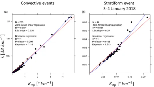
software program that was developed at Colorado State Uni-versity by Chenxiang Tang and Viswanathan N. Bringi. The raw Parsivel2DSD measurements have a time resolution of 1 min. The volumetric concentrations were computed with a 5 min resolution and binned into 32 diameter classes with in-creasing sizes from 0.125 mm up to 6 mm. The CANTMAT software uses the T-matrix formulation to compute radar ob-servables such as horizontal reflectivity, vertical reflectivity, differential reflectivity, copolar cross-correlation, specific at-tenuation, specific phase shift, etc., as a function of the DSD, the radar frequency, air temperature, oblateness models (e.g., Beard and Chuang, 1987; Andsager et al., 1999; Thurai and Bringi, 2005), and canting models for the rain drops and the incidence angle of the electromagnetic waves. Figure 8 dis-plays the empirical k–Kdp pairs of points obtained for the
convective events (left) and the stratiform one (right) as well as the fits of least square linear models and power law non-linear regressions.
Based on the literature review mentioning an almost linear relationship between k and Kdpat X band (Bringi and
Chan-drasekar, 2001; Testud et al., 2000; Schneebeli and Berne, 2012), we have first tested a linear regression with an inter-cept forced to be equal to 0 (red lines in Fig. 8). This simple model provides a rather good fit to the data, especially for the convective events. Due to the observed bending of the scatterplots, we have also tested a nonlinear regression to a power law model (blue curve) which significantly improves the fittings. A sensitivity analysis was performed in order to test the influence of the raindrop temperature, the raindrop oblateness model, the standard deviation of the canting angle distribution and the incidence angle. For reasonable ranges of the variation of these parameters, the DSD itself appears to be the most influential factor on the values of the regression coefficients. We note that the slopes of our zero-forced lin-ear models are significantly higher than the values proposed in the literature (0.233 in Bringi and Chandrasekar, 2001; 0.205–0.245 in Scheebeli and Berne, 2012). The exponents of the fitted power law models are also significantly higher than 1.0. The fits in Fig. 8 correspond to the most likely pa-rameterization of the scattering model in terms of tempera-ture and incidence angles for the two events, i.e., 20◦C and 7.5◦, respectively, for the convective cases and 0◦C and 0◦ for the stratiform case. The Beard and Chuang (1987) formu-lation was used as the raindrop oblateness model. The DSD-derived linear and nonlinear k–Kdp relationships were used
to process the regularized φdp(r) profiles which were first
simply derived to obtain the Kdp(r)profiles prior to the
ap-plication of the two k–Kdprelationships. The bottom graphs
of Fig. 5 show examples of the resulting polarimetry-derived PIAs.
4 Results
4.1 Study of the φdp–PIA relationship in rain
Figure 9 displays the scatterplot of the φdp–PIA values
ob-tained for the nine convective events (Table 2) with the XPORT 7.5◦PPI data, following the methodology described in Sect. 3.1 and 3.2. The data from the 16 mountain targets (Table 3) were considered. For a given event, targets with maximum MRT-derived PIAs less than 5 dB were discarded in order to limit the weight of small PIA estimates in the global analysis. Since we consider the two variables to be on an equal footing, we preferred to calculate the least rectan-gles regression (blue straight line) between the two variables rather than the least squares regression of one variable over the other one. One can notice the rather large dispersion of the scatterplot with an explained variance of 77 %. We note the regression slope (0.41) to be higher than the slope of the k–Kdp linear relationship (0.336), which is reported as the
red straight line in Fig. 9.
To go further, Fig. 10 presents the comparison of the MRT-derived PIAs with the polarimetry-MRT-derived PIAs. The linear k–Kdp relationship leads to a significant positive bias for
the polarimetry-derived PIAs with a least rectangles slope of 1.24. The nonlinear k–Kdprelationship does a good job of
reducing this bias (least rectangles slope of 1.03). This result may be surprising given the k–Kdp relationships displayed
in Fig. 8. One has to realize that the range of Kdp values
is much smaller for the 5 min DSD estimations than for the Kdp(r)profiles discretized with a 34.2 m resolution.
Consid-ering that the 1 min DSDs allowed us to confirm the validity of the linear and nonlinear k–Kdp models for a wider Kdp
range (not shown here for the sake of conciseness), we are therefore confident in the relevance of the results presented in Fig. 10.
4.2 Study of the ψdp–PIA relationship in the melting
layer
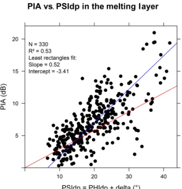
Figure 11 displays the scatterplot of the φdp–PIA values
ob-tained in the ML for the 4 January 2018 stratiform event with the MOUC 0◦ PPI data, following the methodology described in Sect. 3.1 and 3.2. The results obtained for the 13 targets (Table 4) are considered in this analysis, with no target censoring based, for instance, on the minimum PIA observed for a given target as for the XPORT case study. One can see that the correlation between the two vari-ables is severely degraded compared to the rain case with an explained variance of 41 % and a least rectangle slope of 0.51 dB per degree. The red line recalls the k–Kdplinear
re-gression determined with the DSDs observed at ground level for this event. Clearly, the φdp–PIA relationship is different
in rain and in the ML and, as suggested when commenting on Fig. 6, it likely depends on the physical processes occurring during the melting.
Figure 8. DSD-derived k–Kdprelationships for the nine convective events (a) and for the stratiform event of 3–4 January 2018 (b) (see text for details).
Figure 9. PIA–φdpscatterplot for the nine convective events consid-ered in this study. The blue line corresponds to the least rectangle fit to the data, while the red line corresponds to the linear k–Kdp relationship derived from the DSD data available at ground level.
To investigate this point, φdp(rM)and PIA(rM)values
es-timated during the rising of the ML at the level of the MOUC radar are represented in Fig. 12 as a function of their position within the ML. As already noted, we define the ML width as the difference between the Zh top altitude and the ρhv
bot-tom altitude (Khanal et al., 2019). Since the ML width sig-nificantly varies during the considered period (from 630 to 1020 m; see Fig. 8), we found it necessary to scale the
alti-tudes by the ML width. This was achieved by considering the following linear transformation of the altitudes:
H (t ) = (hM−hρhvB(t ))/MLw(t ), (4)
where hM is the altitude (m a.s.l.) of the MOUC radar,
hρhvB(t )is the altitude of the ML bottom and MLw(t ) is the
ML thickness at a given time t . The scaled altitude H (t ) [–] subsequently takes the value 0 at ML bottom and the value 1 at ML top (orange and blue thick horizontal lines, respec-tively, in Fig. 12). Furthermore, in order to locate more pre-cisely the position of the Zhand ρhv peaks within the ML,
we computed their scaled altitudes at each time step, HzhP(t )
and HρhvP(t ), respectively, as follows:
HzhP(t ) = (hzhP(t ) − hρhvB(t ))/MLw(t ) (5)
and
HρhvP(t ) = (hρhvP(t ) − hρhvB(t ))/MLw(t ), (6)
where hzhP(t )and hρhvP(t )are the altitudes of Zhpeak and
ρhvpeak at time t . The broken horizontal lines in Fig. 12
rep-resent the 10 % and 90 % quantiles of the time series of the scaled altitudes of Zhpeak (broken blue lines) and ρhvpeak
(broken orange lines). We can observe a shift between the Zh
and ρhv characteristic altitudes, consistent with the ML
cli-matology established by Khanal et al. (2019) who reported a shift of about 100 m in average between the two peaks. We note in Fig. 8 that this shift is visible during the snowfall period and at the beginning of the ML rising but that it is less pronounced after 03:00 UTC and during the rainfall pe-riod. In order to better evidence their vertical trends, the MRT PIA (rM)and φdp(rM)values are presented in Fig. 12 as a
function of the scaled altitudes in the form of boxplots with a scaled altitude class of size 0.1. The number of counts in each
Figure 10. Comparison of the PIAs derived from the mountain reference technique and from polarimetry using the linear k–Kdp relation-ship (a) and the nonlinear k–Kdprelationship (b) for the nine convective events. The blue line corresponds to the least rectangle fit to the data and the red line is the 1/1 line.
Figure 11. PIA–φdpscatterplot in the ML for the stratiform event of 3–4 January 2018. The blue line corresponds to the least rectangle fit to the data, while the red line corresponds to the linear k–Kdp relationship derived from the DSD data available at ground level.
class is indicated on the right of the graphs; it is a multiple of the number of MRT targets (13 here) depending on the time occurrence of estimates in a given altitude class. The verti-cal sampling is not very rich, with missing classes within the ML. However, there is a clear signature for the two variables in the ML. The trends already evoked when commenting on Fig. 8 are confirmed as follows: (i) the MRT PIAs peak when measurements are made at the level of the Zhand ρhvpeaks
– more precisely, the PIA peak is observed for the altitude class containing the ρhvpeaks (scaled altitude class centered
at 0.3); (ii) the region with maximum values is somewhat thicker for φdp, encompassing a significant part of the upper
ML, between the 0.3 and 0.8 scaled altitude classes; (iii) φdp
tends towards almost similar values on average in rain (ML bottom) and snow (ML top); and (iv) the PIA tends towards its value in rain below the ML and towards 0 above the ML. One would have expected a more pronounced return towards 0 of the PIAs on top of the ML. This lower-than-expected de-crease could sign a radome attenuation; however, the rainfall intensity is low for the considered event, and the radome is equipped with a heating system so that accumulated snow is unlikely. It may also result from a smoothing effect related to nonuniform beam filling. With its 3 dB beamwidth of 1.28◦, the angular resolution of the measurements of the MOUC radar is 447 and 1005 m at distances of 20 and 45 km, re-spectively, which correspond to the minimum and maximum ranges of the considered mountain targets.
Finally, Fig. 13 displays the evolution of the ratio of the mean of the MRT PIA (rM)values over the mean of φdp(rM)
values as a function of the scaled altitudes. The value of the ratio below the ML (0.33) is in rather good agreement with the slope of the linear model established between the spe-cific attenuation k and the spespe-cific differential phase shift Kdp using the DSD measurements in rain available for this
event (0.29; see Fig. 9). Near the ρhv peak, the ratio value
is equal to 0.42. For the three classes of scaled altitude 0.7, 0.8 and 0.9, the ratio is between 0.32 and 0.38, with an ap-parent secondary maximum for the altitude class 0.8. Data with increased vertical resolution would be necessary to con-firm, or not, this observation, which is also visible on the PIA profile and on several φdp and PIA time series like the ones
displayed in Fig. 8. Above the ML, the ratio progressively tends toward 0 at about 300 to 400 m.
Figure 12. Boxplots of the PIA and φdpvalues within the ML as a function of the scaled altitude (a and b, respectively) for the stratiform event of 4 January 2018. The horizontal blue and orange continuous lines represent the ML top and bottom, respectively; the broken horizontal blue and orange lines give the 10 % and 90 % quantiles of the scaled altitudes of the Zhand ρhvpeak distributions, respectively.
Figure 13. Evolution of the ratio of the mean PIAs over the mean ψdpvalues within the ML as a function of the scaled altitudes for the stratiform event of 3–4 January 2018. The horizontal blue and orange lines represent the ML top and bottom, respectively; the bro-ken horizontal blue and orange lines give the 10 % and 90 % quan-tiles of the scaled altitudes of the Zh and ρhv peak distributions, respectively.
5 Summary and conclusions
In this work we developed a methodology for studying the relationship between total differential phase shift (φdp) and
path-integrated attenuation (PIA) at X band. Knowledge of this relationship is critical for the implementation of
attenua-tion correcattenua-tions based on polarimetry. We used the mountain reference technique (MRT) for direct PIA estimations associ-ated with the decrease in strong mountain returns during pre-cipitation events. The MRT sensitivity depends on the time variability of the dry weather mountain returns. The MRT PIAs may be positively biased by on-site attenuation related in particular to radome attenuation and negatively biased by the effect of precipitation falling over the reference targets. The polarimetry PIA estimation is based on the regulariza-tion of the raw ψdp profiles, and their derivation in terms
of specific differential phase shift (Kdp) profiles, followed
by the application of a power law relationship between the specific attenuation and the specific differential phase shift. Such k–Kdprelationships were evaluated for rain with a
scat-tering model by using DSD measurements and an oblateness model for raindrops. The noise of the raw ψdp profiles, the
possible contamination of the signal by differential shift on backscatter and the adequacy of the k–Kdprelationship is the
main factor that determines the quality of the polarimetry-derived PIAs. Nonuniform beam filling (NUBF) effects may also play a role. A point to emphasize is that both PIA esti-mators are not sensitive to an eventual radar miscalibration.
We presented first a rain case study based on nine con-vective events observed with the XPORT radar located in the Grenoble valley. A total of 16 mountain targets were consid-ered with the dry weather mean apparent reflectivity greater than 45 dBZ. The stability of the apparent reflectivity of the mountain targets was shown to be very good, which is an indication of good radar calibration stability during the con-sidered period. The time variability of the reference returns during dry weather preceding or succeeding the rain events was also found to be very small with standard deviations in the range of [0.2–0.9 dBZ], enabling a MRT PIA sensitiv-ity better than 1 dB. Since the XPORT radar is radomeless, on-site attenuation effects are most likely negligible. The
im-pact of rain falling over the mountain targets may also be very limited due to the high reflectivity threshold consid-ered (45 dBZ). The development of the regularization proce-dure of the raw ψdpprofiles required a significant effort, and
we are confident in its ability to deal with the measurement noise, especially for heavy precipitation. We carefully exam-ined many raw and regularized profiles, looking for possi-ble evidence of δhvcontamination during the considered
con-vective events. We found some profiles with rather well or-ganized bumps that could signal such contaminations. The regularization procedure was adapted in order to filter such effects, with a satisfactory performance when they occur at some distance (some kilometers) from the mountain target. In addition, we remind the reader that the observed ψdp(rM)
values extend up to 80◦, while the theoretical δhvrange is 0–
4 dB. The δhveffect may therefore impact the results obtained
only at the margin in the considered case study. NUBF effects may constitute an additional source of error which, although the rain events were convective, should remain limited due to the short ranges considered. In the end, the scatterplot of the MRT PIAs as a function of the φdp(rM)values for all
the nine convective events presents a good coherence overall with, however, a significant dispersion (explained variance of 77 %). It is interesting to note that the nonlinear k–Kdp
rela-tionship derived from independent DSD measurements taken during the events of interest at ground level allows for a satis-factory transformation of the XPORT φdp(rM)values into
al-most unbiased (although dispersed) PIA estimates. Both es-timation methods are prone to specific errors and, even if the MRT PIA estimator is more directly related to power atten-uation, it is a priori difficult to say which estimator is the best. An assessment exercise of attenuation correction algo-rithms, making use of both PIA estimators, with respect to an independent data source (e.g., rain gauge measurements), is desirable to distinguish the two PIA estimators. From this perspective, a specific experiment is being designed within the RadAlp project and it will be implemented in the near future.
The melting layer (ML) case study of 3–4 January 2018 was made possible by the unique configuration of the obser-vation system available. The study of the k–Kdprelationship
within the ML is desirable to better quantify the attenuation effects in the ML with polarimetry; and one has to recognize that such a relationship can still be very difficult to charac-terize theoretically given that scattering models and particle size distributions need to be collected in the ML. The XPORT radar located at the bottom of the valley allowed for a de-tailed temporal tracking of the ML from below using quasi-vertical profiles derived from 25◦ PPIs. The MOUC radar provided horizontal scans at an altitude of 1917 m a.s.l. in the direction of several mountain targets during the rising of the ML in about 2 h. From this dataset, it was possible to derive the evolution of PIA (rM)and φdp(rM)values as a function of
the altitude within the ML. The evolution with the altitude of the ratio of the mean value of PIA (rM)over the mean value
of φdp(rM), as a proxy for the slope of a linear k–Kdp
rela-tionship within the ML, was also considered. Since the ML width varied during the ML rising, we found it necessary to scale the altitudes with respect to the ML width. The three variables considered present a clear signature as a function of the scaled altitude. In particular, the PIA/φdp ratio peaks at
the level of the ρhvpeak (somewhat lower than the Zhpeak),
with a value of 0.42 dB per degree, while its value in rain just below the ML is 0.33 dB per degree. The latter value is con-sistent with the slope of the linear k–Kdprelationship (0.29)
established from concomitant DSD measurements at ground level. The PIA/φdp ratio remains quite strong in the upper
part of the ML, between 0.32 and 0.38 dB per degree, before tending towards 0 above the ML. One would have expected a more pronounced return towards 0 of the PIAs on top of the ML. This lower-than-expected decrease could signal on-site attenuation occurring at the beginning of the ML rise due to the melting of the snow eventually accumulated over the radome; this effect is probably low for the considered event since the snowfall intensity was small and since the radome is heated. It may also result from a smoothing effect related to nonuniform beam filling (angular resolution of 447 and 1005 m for the range of mountain target distances). The δhv
effect is likely to be strong in the ML (up to 4◦), and its rela-tive importance may be quite high in our case study since the PIA range is significantly lower compared to the rain case study, with maximum PIAs of about 15 dB (note also that the sensitivity of the MRT is less than for the XPORT case study since the dry weather variability of the mountain re-turns is higher with standard deviations in the range [0.62– 1.44]). However, we did not find evidence of δhvsignatures
in the raw ψdp(r)profiles, and we are confident in the
abil-ity of the regularization procedure to filter them in a rather satisfactory way if they eventually occur. Although the ex-perimental configuration for the study of attenuation in the ML presents some limitations (e.g., possible radome atten-uation and NUBF effects), the preliminary results presented here will be deepened by processing a dataset of about 30 stratiform events with the presence of the ML at the level of the MOUC radar.
Data availability. Data can be made available by the first author upon request.
Author contributions. GD developed the concept of the article, re-alized the codes and performed the data processing; GD also wrote the article and handled the review process. AKK was involved in the development of the codes (ML identification, Phidp process-ing, etc.); NY shared his experience of the RHytMME radars and provided the MOUC radar data and the preliminary version of the Phidp regularization procedure. FC is a research engineer who has built the XPORT radar and is now responsible for the current updat-ing program and the data acquisition. BB and NG contributed to the article through scientific discussions and amendments to the paper.