A Survey of Surface Reconstruction from Point Clouds

HAL Id: hal-01348404

https://hal.inria.fr/hal-01348404v2

Submitted on 21 Dec 2016

HAL is a multi-disciplinary open access

archive for the deposit and dissemination of

sci-entific research documents, whether they are

pub-lished or not. The documents may come from

teaching and research institutions in France or

L’archive ouverte pluridisciplinaire HAL, est

destinée au dépôt et à la diffusion de documents

scientifiques de niveau recherche, publiés ou non,

émanant des établissements d’enseignement et de

recherche français ou étrangers, des laboratoires

A Survey of Surface Reconstruction from Point Clouds

Matthew Berger, Andrea Tagliasacchi, Lee Seversky, Pierre Alliez, Gael

Guennebaud, Joshua Levine, Andrei Sharf, Claudio Silva

To cite this version:

Matthew Berger, Andrea Tagliasacchi, Lee Seversky, Pierre Alliez, Gael Guennebaud, et al.. A

Sur-vey of Surface Reconstruction from Point Clouds. Computer Graphics Forum, Wiley, 2016, pp.27.

�10.1111/cgf.12802�. �hal-01348404v2�

Volume 0 (1981), Number 0 pp. 1–27 COMPUTER GRAPHICSforum

A Survey of Surface Reconstruction from Point Clouds

Matthew Berger1 Andrea Tagliasacchi2,3 Lee M. Seversky1

Pierre Alliez3 Gaël Guennebaud4 Joshua A. Levine5 Andrei Sharf6 Claudio T. Silva7

1_{Air Force Research Laboratory, Information Directorate} 2_{École Polytechnique Fédérale de Lausanne (EPFL)} 3_{University of Victoria} 4_{Inria Sophia Antipolis-Méditerranée} 5_{Inria Bordeaux Sud-Ouest} 6_{Clemson University}

7_{Ben-Gurion University} 8_{New York University}

Abstract

The area of surface reconstruction has seen substantial progress in the past two decades. The traditional problem addressed by surface reconstruction is to recover the digital representation of a physical shape that has been scanned, where the scanned data contains a wide variety of defects. While much of the earlier work has been focused on reconstructing a piece-wise smooth representation of the original shape, recent work has taken on more specialized priors to address significantly challenging data imperfections, where the reconstruction can take on different representations – not necessarily the explicit geometry. We survey the field of surface reconstruction, and provide a categorization with respect to priors, data imperfections, and reconstruction output. By considering a holistic view of surface reconstruction, we show a detailed characterization of the field, highlight similarities between diverse reconstruction techniques, and provide directions for future work in surface reconstruction.

1. Introduction

Advances made by the computer graphics community have revolutionized our ability to digitally represent the world around us. One subfield that has blossomed during this rev-olution is surface reconstruction. At its core, surface recon-struction is the process by which a 3D object is inferred, or “reconstructed”, from a collection of discrete points that sample the shape. This survey compiles the major directions and progress of the community that addresses variants of the basic problem, and it reflects on how emerging hardware technology, algorithmic innovations, and driving applications are changing the state-of-the-art.

Surface reconstruction came to importance primarily as a result of new techniques to acquire 3D point clouds. Early on, these technologies ranged from active methods such as optical laser-based range scanners, structured light scanners, and LiDAR scanners to passive methods such as multi-view stereo. These devices fundamentally changed the way we ac-complished engineering and rapid prototyping tasks, and they have improved hand-in-hand with technologies for computer-aided design.

Computer graphics took an immediate interest in such tech-nology, following one of its longstanding goals: the modeling,

recognition, and analysis of the real world. Moreover, current applications have made use of such scanners in all fields of data-driven science, spanning from the micro- to macro-scale. A more recent trend has seen the massive proliferation of point clouds from inexpensive commodity real-time scan-ners such as the Microsoft Kinect. This has impacted varied fields including automotive design, engineering, archaeology, telecommunications, and art.

In many ways, it is these new acquisition methods that pose the most significant challenge for surface reconstruction. Each distinct method tends to produce point clouds contain-ing a variety of properties and imperfections. These prop-erties, in conjunction with the nature of the scanned shape, effectively distinguish the class of reconstruction methods that exist today. This diverse set of techniques ranges from methods that assume a well-sampled point cloud, generalize to arbitrary shapes, and produce a watertight surface mesh, to methods that make very loose assumptions on the quality of the point cloud, operate on specific classes of shapes, and output a non-mesh based shape representation.

Our survey presents surface reconstruction algorithms from the perspective of priors: assumptions made by algorithms in order to combat imperfections in the point cloud and to

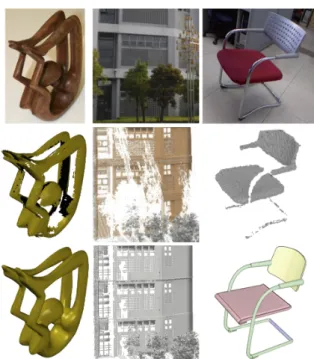
Figure 1: Surface reconstruction has grown in diversity in recent years resulting in techniques taking on specialized priors. ROSA [TZCO09], shown on the left, uses volumetric smoothness to aid in reconstruction. Non-local consolida-tion [ZSW∗_{10], shown in the middle, uses global regularity in}

the form of structural repetition. Part composition [SFCH12], shown on the right, uses data-driven techniques.

eventually focus what information about the shape is re-constructed. Without prior assumptions, the reconstruction problem is ill-posed; an infinite number of surfaces can pass through (or near) a given set of data points. Assumptions are usually imposed on the point cloud itself, such as sampling density, level of noise, and misalignment. But just as impor-tantly they are also imposed on the scanned shape, such as local surface smoothness, volumetric smoothness, absence of boundaries, symmetries, shape primitives, global regularity, and data-driven assumptions. In some instances, requirements are made on knowledge of the acquisition, such as scanner head position, as well as RGB images of the object. In other cases, the user is involved in prescribing high-level cues for reconstruction. All of these factors permit the regularization of the otherwise ill-posed problem of surface reconstruction, particularly when processing a point cloud containing severe imperfections. Figure1depicts several different priors used to reconstruct surfaces from challenging point clouds. The utility of classifying surface reconstruction in terms of priors also helps to constrain expectations and prioritize de-sirables for reconstruction output in application dependent ways. For example, in the field of archaeology, dense, good-coverage scans might be available (e.g. the Digital

Michae-langelo project [LPC∗_{00]), allowing for standard smoothness}

priors that enable the high-detail reconstruction. Such great detail enables more than just digitization, but also the preser-vation of culture in ways that will transform how we study art [SCC∗_{11]. In urban planning, reconstructing fine details}

such as individual bricks on a building might be both unnec-essary and impossible given incomplete terrestrial LiDAR scans. However, in such contexts global regularity priors en-able detail completion as well as interactive, realistic proxies for missing details such as plants and vegetation [BAMJ∗_11].

Historically, priors have evolved in conjunction with the types of point clouds being processed. For instance, surface smooth-ness priors were developed primarily to handle small objects acquired from desktop scanners. Mobile, real-time scanners have enabled the dynamic acquisition of more general scenes, rather than single objects, prompting more specialized struc-tural and data-driven priors. Since priors tend to be coupled with the type of acquisition, we argue that our perspective of surface reconstruction is beneficial for understanding how to process future types of acquired point clouds.

Organization. Our survey is organized as follows. Sec-tions2–3provide background on surface reconstruction. In Section2we examine the basic characteristics of a recon-struction algorithm, namely:

• Point Cloud Artifacts: the imperfections of the point cloud that the method is able to effectively handle. • Input Requirements: the types of inputs associated with

a point cloud required by the algorithm.

Section3provides an overview of the different priors from the perspective of the type of data produced through acquisi-tion, the shape classes that tend to be acquired, and the type of output produced. We use all of these considerations as a way of examining surface reconstruction methods, starting with traditional surface smoothness priors in Section4, and delving into specialized priors in Sections5–10. In Table1.1

we provide a summary of surface reconstruction methods by prior, characterizing their input and output, as well as their level of robustness to various artifacts. We discuss meth-ods for evaluating surface reconstruction in Section11, and conclude in Section12with a discussion on future trends. 1.1. Survey Scope and Related Works

There are many variants to surface reconstruction. This sur-vey focuses on those relating to the reconstruction from point clouds of static objects and scenes acquired through 3D scan-ners, wherein the point cloud contains a considerable level of imperfection. Furthermore, we concentrate on methods that approximate the input point cloud. For clarity, we contrast this organization relative to other important types of surface reconstruction:

Urban reconstruction. Our survey covers a wide variety of reconstruction methods, with urban reconstruction from

Method Point Cloud Artifacts Input Requirements Shape Class Reconstruction Output

nonuniform sampling noise outliers misalignment missing

data

unoriented normals oriented normals scanner information RGB

image

Surface Smoothness Tangent Planes [HDD∗_92]

# # general implicit field

RBF [CBC∗_01]

# # 3 general implicit field

MLS [ABCO∗_03]

# # 3 general point set

MPU [OBA∗_03]

# # # 3 general implicit field Poisson [KBH06] # # # # 3 general implicit field Graph Cut [HK06] # # # # # general volumetric segmentation Unoriented Indicator [ACSTD07] # # # # 3 general implicit field

LOP [LCOLTE07] # # general point set Dictionary Learning [XZZ∗_14]

# general mesh

Visibility

VRIP [CL96] # # 3 general implicit field TVL1-VRIP [ZPB07] # # # # 3 general implicit field Signing the Unsigned [MDGD∗_10]

# # 3 general implicit field

Cone Carving [SSZCO10] # # 3 3 general implicit field Multi-Scale Scan Merge [FG11] # 3 general implicit field

Volumetric smoothness

ROSA [TZCO09] # # 3 organic skeleton curve Arterial Snakes [LLZM10] # # 3 man-made skeleton curve VASE [TOZ∗_{11] # # 3 general implicit field}

l1Skeleton [HWCO∗13] # # organic skeleton curve Geometric Primitives

Primitive Completion [SDK09] # # # 3 CAD volumetric segmentation Volume Primitives [XF12] # # # 3 indoor environment interior volume Point Restructuring [LA13] # # # # # 3 3 general volumetric segmentation

CCDT [vKvLV13] # # # # 3 3 urban environment volumetric segmentation Global Regularity

Symmetry [PMW∗_08]

# # 3 architectural point set Nonlocal Consolidation [ZSW∗_10]

# # 3 architectural point set 2D-3D Facades [LZS∗_11]

# # 3 3 architectural point set Globfit [LWC∗_11]

# 3 man-made primitive relations RAPter [MMBM15] # # indoor environment primitive relations

Data-driven

Completion by Example [PMG∗_{05] # # 3 general point set}

Semantic Modeling [SXZ∗_12]

# # 3 3 indoor scene objects deformed model Shape Variability [KMYG12] # # 3 indoor scene objects deformed model Part Composition [SFCH12] # # 3 3 man-made deformed model parts

Interactive Topological Scribble [SLS∗_07]

# # 3 general implicit field

Smartboxes [NSZ∗_10]

# # 3 architectural primitive shapes O-Snap [ASF∗_13]

# # # 3 architectural primitive shapes Morfit [YHZ∗_14]

# # general skeleton + mesh

Table 1: A categorization of surface reconstruction in terms of the type of priors used, the ability to handle point cloud artifacts, input requirements, shape class, and reconstruction output. Here # indicates that the method is moderately robust to a particular artifact and indicates that the method is very robust. 3indicates an input requirement and 3indicates optional input. point clouds among them. We note that [MWA∗_{13] surveys}

urban reconstruction more broadly: 3D reconstruction from images, image-based facade reconstruction, as well as recon-struction from 3D point clouds. Although there exists some overlap between the body of surveyed material, we cover these methods in a different context, namely the priors that underlay the reconstruction methods and how they address challenges in point cloud reconstruction.

Interpolatory reconstruction. An important field of surface reconstruction methods are those that interpolate a point cloud without any additional information, such as normals or scanner information. Delaunay-based methods are quite common in this area. The basic idea behind these methods is that the reconstructed triangulated surface is formed by a subcomplex of the Delaunay triangulation. A comprehensive survey of these methods is presented in [CG06], as well as the monograph of [Dey07]. A very attractive aspect of such methods is that they come with provable guarantees

in the geometric and sometimes topological quality of the reconstruction provided the sampling of the input surface is sufficiently dense. Nonetheless, these requirements can be too severe for point clouds encountered in the wild, thus rendering the methods impractical for scanned, real-world scenes containing significant imperfections. We do not cover these methods, as our focus on reconstruction emphasizes how challenging artifacts are dealt with, though we note that there are some recent interpolatory approaches which are equipped to handle moderate levels of noise – see [DMSL11] for a scale-space approach to interpolatory reconstruction. Dynamic reconstruction. Another recent advance in scan-ning techniques has enabled the acquisition of point clouds that vary dynamically. These devices promise the ability to capture more than just a single static object, but one that changes over time. Such techniques are still in their infancy, so they have not as yet explored their full range of potential applications. While we focus our survey on the broad

spec-trum of techniques associated with static point clouds, it is interesting to note that already a prior-oriented viewpoint (e.g. incompressibility [SAL∗_{08] and gradual change [PSDB}∗_10])

has fueled a better understanding of shape in space-time. Single-view reconstruction from images. Very recent work has considered the problem of surface reconstruction from single RGB images [SHM∗_{14,HWK15]. These techniques}

are data-driven, in that they rely on large shape collections to estimate either depth or a full 3D model strictly from a single image. Due to the rapid growth in this new area, and the fact that our primary focus is on reconstruction from point clouds, we have decided not to cover this area in the survey. 2. Surface Reconstruction Fundamentals

Surface reconstruction methods must handle various types of imperfections and make certain requirements on input associated with the point cloud. Here we summarize these properties in order to cover the basic principles underlying surface reconstruction.

2.1. Point Cloud Artifacts

The properties of the input point cloud are an important fac-tor in understanding the behavior of reconstruction methods. Here we provide a characterization of point clouds according to properties that have the most impact on reconstruction algorithms: sampling density, noise, outliers, misalignment, and missing data. See Figure2for a 2D illustration of these artifacts.

Sampling density. The distribution of the points sampling the surface is referred to as sampling density. Sampling den-sity is important in surface reconstruction for defining a neigh-borhood – a set of points close to a given point which captures the local geometry of the surface, such as its tangent plane. A neighborhood should be large enough so that the points sufficiently describe the local geometry, yet small enough so that local features are preserved. Under uniform sampling density, a neighborhood may be constructed at every point in the same manner. For instance, one can define a neighborhood at a pointp ∈ P via an ε–ball, defined as the set of points Nε(p) ⊂ P such that each y ∈ Nε(p) satisfies kp − yk < ε, under a single valueε used at all points.

3D scans typically produce a nonuniform sampling on the sur-face, where the sampling density spatially varies. This can be due to the distance from the shape to the scanner position, the scanner orientation, as well as the shape’s geometric features. See Figure2(b)for an illustration of nonuniform sampling on a curve. To capture the local variation in sampling density, a common approach is to use the k nearest neighbors (knn) at a given point for neighborhood construction. Another alterna-tive is to use a spatially-varyingε–ball, commonly defined as a function of a point’s knn neighborhood [GG07].

More sophisticated sampling density estimation techniques

(a) Original shape (b) Nonuniform sampling

(c) Noisy data (d) Outliers

(e) Misaligned scans (f) Missing data

Figure 2: Different forms of point cloud artifacts, shown here in the case of a curve in 2D.

use reconstruction error bounds [LCOL06] and kernel meth-ods [WSS09]. The method of [LCOL06] finds the neighbor-hood size at each point by bounding the error of a moving least squares surface approximation [ABCO∗_{03], where the}

selectedε minimizes this error bound. The work of [WSS09] formulates the error of a moving least squares surface ap-proximation in terms of kernel regression, where the optimal neighborhood size may be defined via a point-wise error or the error in the support region of the defined kernel. Noise. Points that are randomly distributed near the surface are traditionally considered to be noise – see Figure2(c). The specific distribution is commonly a function of scanning arti-facts such as sensor noise, depth quantization, and distance or orientation of the surface in relation to the scanner. For some popular scanners, noise is introduced along the line of sight, and can be impacted by surface properties, including scatter-ing characteristics of materials. In the presence of such noise, the typical goal of surface reconstruction algorithms is to pro-duce a surface that passes near the points without overfitting to the noise. Robust algorithms that impose smoothness on the output [KBH06], as well as methods that employ robust statistics [OGG09], are common ways of handling noise. Outliers. Points far from the true surface are classified as out-liers. Outliers are commonly due to structural artifacts in the acquisition process. In some instances, outliers are randomly distributed in the volume, where their density is smaller than the density of the points that sample the surface. Outliers can also be more structured, however, where high density clusters of points exist far from the surface, see Figure2(d). This can occur in multi-view stereo acquition, where view-dependent specularities can result in false correspondences. Unlike noise, outliers are points that should not be used to infer the surface, either explicitly through detection [LCOLTE07], or implicitly through robust methods [MDGD∗_10].

Misalignment. The imperfect registration of range scans re-sults in misalignment, see [vKZHCO11] for a survey on registration techniques. Misalignment tends to occur for a registration algorithm when the initial configuration of a set of range scans is far from the optimal alignment – see Fig-ure2(e)for a 2D illustration. In scanning scenarios where we are only concerned with the acquisition of a single object, it is common for the object to rotate in-place with respect to the sensor for each scan; hence, the amount of misalign-ment is bounded since the initial scan alignmisalign-ment may be estimated from the known rotations. In SLAM-based RGBD-mapping [HKH∗_{12], however, drift can occur. Drift is the}

gradual accumulation of misregistration errors between se-quential scans. This can manifest as substantial misalignment between scans of a single object taken at very different times, a phenomenon known as loop closure.

Imperfections due to misalignment require techniques which differ from handling standard noise. For instance, under a Manhattan world prior [VAB12] a scene is composed of planar primitives aligned along three orthogonal axes – hence planar primitives from erroneously rotated scans can be robustly “snapped” onto one of these axes. Under the prior of repetitive relationships between geometric primi-tives [LWC∗_{11], a misaligned scan can be corrected if it fails}

to conform to the remaining discovered repetitions. Missing data. A motivating factor behind many reconstruc-tion methods is dealing with missing data. Missing data is due to such factors as limited sensor range, high light absorption, and occlusions in the scanning process where large portions of the shape are not sampled. Although the aforementioned artifacts are continually improved upon, missing data tends to persist due to the physical constraints of the device. We note that missing data differs from nonuniform sampling, as the sampling density is zero in such regions – see Figure2(f). Many methods deal with missing data by assuming that the scanned shape is watertight [CBC∗_{01,Kaz05,KBH06,HK06,}

ACSTD07]. Here the goal can be to handle the aforemen-tioned challenges where data exists, and infer geometry in parts of the surface that have not been sampled. Other meth-ods are focused on handling missing data by trying to infer topological structures in the original surface at the possible expense of retaining geometric fidelity, for instance, finding a surface that is homeomorphic to the original shape [SLS∗_07].

For significant missing data, other approaches seek the re-construction of higher-level information such as a skele-ton [TZCO09], shape primitives [SDK09], symmetry rela-tionships [PMW∗_{08], and canonical regularities [LWC}∗_11].

2.2. Point Cloud Input

Reconstruction methods have different types of input require-ments associated with a point cloud. The bare minimum requirement of all algorithms is a set of 3D points that sample the surface. Working with the points alone, however, may

fail to sufficiently regularize the problem of reconstruction for certain types of point clouds. Other types of input can be extremely beneficial in reconstruction from challenging point clouds. We consider the following basic forms of inputs com-monly associated with point clouds: surface normals, scanner information, and RGB imagery.

2.2.1. Surface Normals

Surface normals are an extremely useful input for recon-struction methods. For smooth surfaces the normal, uniquely defined at every point, is the direction perpendicular to the point’s tangent space. The tangent space intuitively represents a localized surface approximation at a given point. Surface normals may be oriented, where each normal is consistently pointing inside or outside of the surface, or may lack such a direction. Normals that are oriented provide extremely useful cues for reconstruction algorithms – see [CBC∗_01,KBH06].

Unoriented normals. Normals that do not possess direction – the input normal at every point can be expected to be point-ing either in the inside or the outside of the surface – are considered to be unoriented normals. This information can be used in a number of ways: determining planar regions in a point cloud [SWK07], the projection of a point onto an approximation of the surface [ABCO∗_{03], or the construction}

of an unsigned distance field [AK04].

Unoriented normals are typically computed directly from the point cloud alone. A popular and simple method for comput-ing the normal at a given pointp ∈ P is to perform principal component analysis (PCA) in a local neighborhood ofp. The method of [HDD∗_{92] estimates the normal as the smallest}

eigenvector of the covariance matrix constructed over a local neighborhood of points, obtained via anε-ball or its k nearest neighbors. PCA defines a total least-squares plane fitting es-timation of the tangent plane, and as such can be sensitive to imperfections in the point cloud, such as the sampling density and noise. The work of [MNG04] analyzes the accuracy of this form of normal estimation, where they show that the an-gle between the true normaln and the PCA-estimated normal ˆn, with probability 1 − ε, is:

^(n, ˆn)≤ C1κr +C2_r2σ√ερ +Cn 3σ 2 n

r2, (1)

whereκ is the curvature at p, r is the radius for the r–ball used in constructing the neighborhood,σnis the noise magnitude

under zero-mean i.i.d. noise,ρ is the sampling density, and C₁, C₂, and C₃are constants independent of these quantities. Note the trade-off between noise and the neighborhood size: asσnvanishes, r should be small, but as noise is introduced,

r should be large in order to combat the effects of noise. Other methods for normal estimation consist of using a weighted covariance matrix [PMG04] and higher-order ap-proximations via osculating jets [CP05]. Similar to standard PCA, these methods require a local neighborhood of points, hence in the presence of point cloud imperfections it can

be quite challenging to find the optimal neighborhood. As a result, these estimation methods can produce rather noisy normals, and so reconstruction algorithms must be robust to this.

Oriented normals. Normals that have consistent directions, either pointing in the inside or the outside of the surface are referred to as being oriented. Knowledge of the exterior and interior of the surface has proven extremely useful in surface reconstruction. It can be used to construct a signed distance field over the ambient space, where up to a sign, the field takes on positive values in the exterior and negative values in the interior. The surface is then represented by the zero crossing of the signed distance field. Other methods generalize this to implicit fields and indicator functions, but the basic idea of trying to construct the exterior and interior remains the same, see [CBC∗_01,OBA∗_{03,KBH06] to name a few.}

There are numerous ways to compute oriented normals. If the original 2D range scans are known, then the 2D lattice structure provides a way of performing consistent orientation since one always knows how to turn clockwise around a given vertex. For instance, if we denote the point in a range scan at pixel (x,y) aspx,y, then one can take the normal at

px,ysimply as the cross product between (px+1,y− px,y)and (px,y+1− px,y). If the point cloud is noisy, then this method

can produce rather noisy normals, since it does not aggregate points in overlapping scans.

If scanner information is absent altogether, then one must ori-ent the points exclusively from the unoriori-ented normals. The well-known method of [HDD∗_{92] achieves this by}

construct-ing a graph over the point cloud (e.g. through each point’s knn neighborhood) and weights each edge wi jfor pointspi

andpjbased on the similarity between the respective points’

unoriented normalsniandnjas wi j=1−|ni·nj|. A minimal

spanning tree is then built, where upon fixing a normal orien-tation at a single point serving as the root, normal orienorien-tation is propagated over the tree. The method of [HLZ∗_{09] adjusts}

the weights wi jby prioritizing propagation along tangential

directions – if the estimated tangent space between two points pi− pjis perpendicular to the normal directions, then this

indicates these two points are valid neighbors, rather than belonging to opposite sides of the surface.

Although these methods are able to deal with nonuniform sampling, noise, and misalignment to a certain degree, they still remain sensitive to imperfections in the point cloud, and as a result can leave some normals unoriented or pointing in the wrong direction – see Figure3. The impact on surface reconstruction largely depends on the distribution of incorrect orientations: if randomly distributed, then methods may treat this as spurious noise, but if incorrect orientations are clus-tered together over large regions, then this form of structured noise can be difficult to handle.

Figure 3: The impact of incorrect normal orientation. On the left we show the result of normal orientation via [HDD∗_92],

where red splats indicate incorrect orientation. The results of running Poisson surface reconstruction [KBH06] on this point cloud are shown in mid-left, where we indicate un-wanted surface components due to the clustered normal flips. Similarly, on the right we show the orientation results of [LW10], and the corresponding results of [KBH06].

2.2.2. Scanner Information

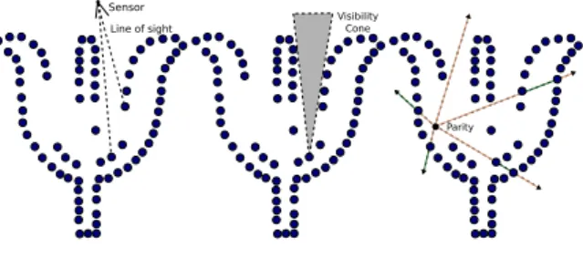
The scanner from which the point cloud was acquired can provide useful information for surface reconstruction. Its 2D lattice structure permits the estimation of sampling density which can be used to detect certain forms of outliers – points whose lattice neighbors are at a far greater distance than the sampling density are likely outliers. However, caution must be taken in distinguishing outliers from sharp features. Scanner information may also be used to define the confi-dence of a point, which is useful in handling noise. Certain scanners (e.g. LiDAR) provide confidence measures in the form of the reflectivity measured at each point. One can also derive confidence through line of sight information. Line of sight is the collection of line segments between each point in the point cloud and the scanner head position from which that point was acquired. In active scanning systems, i.e. laser-based scanners, if the angle between the line of sight and the surface normal is large, this can result in noisy depth estimation, i.e. poor laser peak estimation [CL96], implying low confidence.

Note that line of sight also defines a region of space marked as lying outside of the shape. Combining line of sight from mul-tiple scans refines the bounding volume in which the surface lies – this is known as the visual hull. This information is par-ticularly useful when handling incomplete data – it can infer that there exists a large concavity in the shape [TOZ∗_11].

2.2.3. RGB Imagery

Different acquisition modalities that complement depth ac-quisition can be of great assistance. RGB image acac-quisition is a very common modality that accompanies numerous sen-sors, such as the Microsoft Kinect. In the case of the Kinect, the RGB camera is co-located with the IR camera, hence assuming the two are calibrated, it is straightforward to iden-tify corresponding depth and RGB values at a pixel level.

RGB images are most useful for reconstruction when they are able to complement depth information that is either not as descriptive as its visual appearance, or simply not measured by the data. For instance, if a color image and 3D scan are at a wide baseline, hence containing very different views, then segmented parts of the image can be used to infer 3D geometry in the original scan [NSC14].

3. The Role of Priors

The development of priors is largely driven by emerging data acquisition technologies. Acquisition methods set expecta-tions for the class of shapes that can be acquired and the type of artifacts associated with the acquired data, consequently informing the type of output produced by reconstruction al-gorithms and the fidelity of the reconstruction. In this section we provide an overview of each prior, discussing the type of inputs each prior expects and subsequent output produced, as well as the typical shape classes and acquisition methods that characterize these scenarios.

3.1. Surface Smoothness

The surface smoothness prior constrains the reconstructed surface to satisfy a certain level of smoothness, while en-suring the reconstruction is a close fit to the data. Perhaps the most general form is local smoothness, which strives for smoothness only in close proximity to the data. The output of such approaches are typically surfaces that smooth out noise associated with the acquisition, while retaining bound-ary components where there exists insufficient sampling (or simply no sampling) [HDD∗_92,ABCO∗_{03]. Due to their}

gen-erality, these methods can be applied to many shapes and acquisition devices, yet absent of additional assumptions, handling severe artifacts poses a significant challenge. In contrast, global smoothness seeks higher order smooth-ness, large-scale smoothsmooth-ness, or both. High order smoothness relates to the variation of differential properties of the sur-face: area, tangent plane, curvature, etc. Large-scale herein relates to the spatial scale where smoothness is enforced – not just near the input. It is common for these methods to focus on reconstructing individual objects, producing water-tight surfaces [CBC∗_{01,KBH06]. As a result, this limits the}

class of shapes to objects that can be aquired from multiple views, captured as completely as possible. Desktop scan-ners capable of scanning small (i.e. 1 inch) to mid-sized (i.e. several feet) objects are commonly used to produce such point clouds. Laser-based optical triangulation scanners, time-of-flight (TOF) scanners, and IR-based structured lighting scanners are all representative devices for such scenarios. Furthermore, due to the sensor’s close proximity to an object and its high resolution capabilities, an emphasis is commonly placed on reconstructing very fine-grained detail.

Piecewise smooth priors seek to preserve sharp (i.e. nons-mooth) features in the shape [FCOS05,ASGCO10]. For this

prior the acquisition device does not differ much from global or local smoothness priors, but rather the class of shapes are restricted to those which contain a set of sharp features – i.e. CAD models, man-made structures, etc.. Surface smoothness priors are covered in detail in Section4.

3.2. Visibility

The visibility prior makes assumptions on the exterior space of the reconstructed scene, and how this can provide cues for combating noise, nonuniform sampling, and missing data. Scanner visibility is a powerful prior, as discussed in Sec-tion2.2.2, as it can provide for an acquisition-dependent noise model and be used to infer empty regions of space [CL96]. This enables the filtering of strong, structured noise – a com-mon characteristic of multi-view stereo outputs – for water-tight reconstruction of individual objects [ZPB07]. Recent work has extended the visibility prior to scene reconstruction in an interactive setting by relaxing the watertight constraint and only maintaining a surface in close proximity to the data [NDI∗_{11]. The Microsoft Kinect and Intel’s RealSense}

are two representative scanners which enable the interactive acquisition of geometry. Such scanners permit the reconstruc-tion of very large spaces, i.e. building interiors, but often at the expense of geometric fidelity compared to static, more constrained scanning setups. Methods which employ visibil-ity priors are discussed in more detail in Section5.

3.3. Volume Smoothness

The volume smoothness prior imposes smoothness with re-spect to variations in the shape’s volume. This has shown to be quite effective when faced with large amounts of miss-ing data [TZCO09,LYO∗_{10]. Some volume priors assume}

the watertight reconstruction of an individual object with an emphasis on topological accuracy, where it is assumed that the well-sampled acquisition of an object is prohibited, pri-marily due to self-occlusions and limited mobility in sensor placement. This can be seen in man-made objects composed of such materials as coils or metal wires, where the shape can be described as a complex arrangement of generalized cylinders [LLZM10]. Other techniques such as [LYO∗_10]

focus on extracting the skeleton structure of a shape from sig-nificant missing data. This can be seen in organic shapes, in particular trees, which tend to be scanned via LiDAR sensors in uncontrolled outdoor environments, and as a result many branches and leaves may only be partially scanned. Volume smoothness methods are covered in Section6.

3.4. Primitives

The geometric primitive prior assumes that the scene geome-try may be explained by a compact set of simple geometric shapes, i.e. planes, boxes, spheres, cylinders, etc.. In cases

where we are concerned with watertight reconstruction of in-dividual objects, the detection of primitives [SWK07] can sub-sequently be used for primitive extrapolation for reconstruc-tion when faced with large amounts of missing data [SDK09]. CAD shapes naturally fit this type of assumption since they are usually modeled through simpler geometric shapes, how-ever once scanned, the point clouds may be highly incomplete due to complex self occlusions. Furthermore, certain CAD models are mechanical parts whose physical materials may be unfavorable for scanning with many devices (be it IR, TOF, etc..), hence structured noise may result. The primitive prior can thus be useful for robustly finding the simpler shapes un-derlying the noise-contaminated point cloud [SWK07]. Note, however, that any fine-grained details are likely to be treated as noise with the primitive prior, if they are unable to be represented as a union of smaller primitives.

Indoor environments are another shape class ideal for primi-tives, as they may be summarized as a collection of planes or boxes. A typical application of this is in the reconstruction of a floor plan of a building. Such environments may be captured by LiDAR scanners [XF12], where obtaining full scans can be difficult due to large-scale scene coverage. Hence planes can be a useful prior for completion from incomplete data, in addition to denoising [JKS08,XF12]. Similar to CAD shapes, however, fine geometric details may be lost as a result, though hybrid methods have been developed to preserve detail while simultaneously extracting primitives [LA13,vKvLV13]. Prim-itive prior methods are discussed in detail in Section7. 3.5. Global Regularity

The global regularity prior takes advantage of the fact that many shapes – CAD models, man-made shapes and archi-tectural shapes – possess a certain level of regularity in their higher-level composition. Regularity in a shape can take many forms, such as a building composed of facade elements, build-ing interiors composed of regular shape arrangements, or a mechanical part consisting of recurring orientation relation-ships between sub-parts.

For instance, facades can often be described in terms of re-peating parts, for instance a collection of windows, where the parts possess some regularity in their arrangement, i.e. a uniformly-spaced grid of windows. Facade acquisition, how-ever, is often faced with substantial noise and incomplete measurements, as typical acquisition devices – i.e. LiDAR or multi-view stereo – can only take measurements at far distances and suffer from occlusion with parts of the environ-ment. Hence, if such regularity was detected in the input data, it can be used to model the rest of the facade for denoising and filling in missing parts [ZSW∗_10,LZS∗_11].

A major artifact addressed by global regularity in building interiors and mechanical parts is scan misalignment. For in-stance, building interiors may be captured by the registra-tion of depth scans in real-time scanning devices, but im-perfections in the registration can manifest in drifting, see

Section2.1on misalignment. Enforcing regularity on angles between detected planes can be highly beneficial in correcting for drift [OLA15,MMBM15]. The acquisition of mechanical parts through standard desktop 3D scanners can similarly result in poorly registered depth scans, yet finding canon-ical relationships in extracted geometric primitives can be useful in correcting for these errors [LWC∗_{11]. For}

mechan-ical parts, it is common for the reconstruction objective to produce a watertight reconstruction of an individual object, whereas for building interiors the objective is primarily plane detection, not necessarily a watertight reconstruction. How-ever, due to the large scale of building interiors, there may exist more evidence for regularity compared to a mechanical part, whose small size inherently limits the potential num-ber of relationships, so we see a trade-off in reconstruction fidelity and regularity. Global regularity methods are covered in detail in Section8.

3.6. Data Driven

The data driven prior exploits the large-scale availability of acquired or modeled 3D data, primarily in scenarios where the input point cloud is highly incomplete. In these scenar-ios we are primarily focused on reconstruction of individual objects, or a collection of objects, since 3D databases tend to be populated with well-defined semantic object classes. For instance, we may be concerned with obtaining a wa-tertight reconstruction of an individual object from only a single, or several, depth scans. A database of objects may be used to best match the incomplete point cloud to a complete model [PMG∗_{05], or a composition of parts from different}

models [SFCH12]. In other cases we may be concerned with scene reconstruction, and using the database to complement the detected objects in the scene [SXZ∗_12,KMHG13].

Due to the generality of a data driven prior – the reconstruc-tion quality is as good as the provided data – these methods can be applied to a wide variety of data acquisition scenar-ios and shape classes. Employing complete 3D models for reconstruction poses few limitations, so long as these mod-els accurately reflect the scanned data. If not, then complex nonrigid registration methods are necessary to deform the models appropriately [NXS12,KMYG12]. Employing parts from different models can significantly expand the generaliza-tion of a model database to the input, however this assumes certain shape classes that can be described with respect to well-defined parts: most man-made objects fit this description, but organic shapes may be difficult to describe in terms of parts. To address this, an alternative data-driven prior is to use a shape space, or a compact means of representing shape vari-ations, for which the input data should conform to. This prior can enable the reconstruction of more general scenes, not just individual objects but natural environments consisting of trees [BNB13] or flowers [ZYFY14]. Data driven methods are discussed in Section9.

3.7. User Driven

The user driven prior incorporates the user into the process of surface reconstruction, allowing for them to provide intu-itive and useful cues for reconstruction. The specific form of interaction is largely driven by the type of shape being reconstructed, and how it was acquired. In performing wa-tertight reconstruction of individual objects, often the focus is on topology recovery due to incomplete sampling from the sensor. Hence certain approaches focus on reconstruction of arbitrary shapes [SLS∗_{07], while others admit}

interac-tion with a shape’s skeletal model, relying on the volumetric smoothness prior to guide the reconstruction [YHZ∗_{14]. In}

the reconstruction of architectural buildings, similar to the case of facades discussed in Section3.5, scanning in outdoor environments can cause large gaps in the acquisition. Hence, user interaction can help in the discovery of global regularity, as well as how to apply the detected regularity to the rest of the point cloud [NSZ∗_{10]. If finer-grained control of the}

reconstruction is desired, then the user can specify geomet-ric primitives to model the building, with guidance provided by the relationships discovered in the input [ASF∗_{13]. User}

driven methods are covered in detail in Section10. 4. Surface Smoothness Priors

The surface smoothness prior can roughly be divided into local smoothness, global smoothness, and piecewise smooth-ness. These methods primarily vary based on the smoothness constraint and how it is prescribed in practice.

Notation. We first fix the notation for this section and all subsequent sections. We assume that we are given a point cloud P which is a sampling of a shape S. Individual points in P are indexed aspi∈ P for the i’th point. Many methods

also require normals associated with the point cloud, where we define the normal field N as a set of normal vectors such that for eachpi∈ P there is an accompanying normal ni∈ N.

The distinction between oriented and unoriented normals is made explicit for each method.

4.1. Local Surface Smoothness Priors

The pioneering method of [HDD∗_{92] was hugely influential}

on the class of methods that impose local smoothness priors. This method approximates a signed distance fieldΦ : R3_{→ R}

by assigning, for each point in the ambient spacex ∈ R3_{, its}

signed projection onto the tangent plane of its closest point to P, denotedpi:

Φ(x) = (x − pi)· ni. (2) Note that the normal field N must be oriented in order to obtain an estimate of the signed distance field. The surface is then defined by the zero level set ofΦ. Although straightfor-ward to implement, this approach suffers from several issues. The method is very sensitive to the estimated normals – noisy normals, or worse inverted normal orientations, can give rise

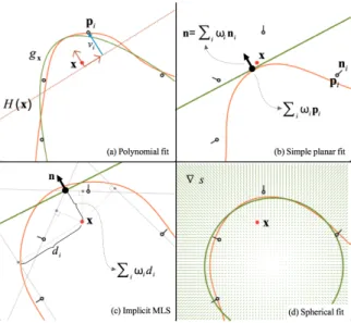
Figure 4: Illustration in 2D of the principle of many MLS surface variants. The local approximations computed for the evaluation pointx in red are show in green. The orange curves correspond to the reconstructed iso-contours.

to very inaccurate signed distance estimates. Furthermore, in the presence of nonuniform sampling, choosing the clos-est tangent plane to define a signed projection can produce a rather noisy output. Subsequent methods based on local surface smoothness have focused on addressing such issues. 4.1.1. Moving least squares (MLS)

This class of methods approaches reconstruction by approx-imating the input points as a spatially-varying low-degree polynomial. Assuming that a scalar value viis associated

to each input samplepi, the reconstructed signal atx is then

defined as the value atx of the multivariate polynomial gx

which best approximates the neighborhood ofx in a weighted least-square sense:

gx=argmin

g

∑

_i ω(kx − pik)(g(pi)− vi)

2_{, (3)}

whereω is a smooth decreasing weighting function giving larger influence to samples near the evaluating point. This weighting function plays the role of a low-pass filter. It is an essential ingredient of MLS to combat moderate levels of noise by allowing the weight function to have a larger spatial influence. For nonuniform sampling, it is necessary to define a weight function whose spatial support varies as a function of the sampling density – see Section2.1For surface reconstruction this approach needs to be adapted to address the lack of a natural parameterization for which vicould be

prescribed – see [CWL∗_{08] for a survey on MLS.}

Levin’s method. In the first MLS formulation [Lev03,

(a) (b) (c)

Figure 5: When sampling density is insufficient to resolve local curvature (a), the plane fitting operation employed by moving least squares [AA04] becomes highly unstable (b). APSS [GG07] addresses this by locally fitting spheres instead of planes. Using spheres tackles the aforementioned problem while remaining computationally inexpensive.

x are first parameterized with respect to a local tangent plane H(x) obtained through a weighted PCA as in normal estima-tion methods (Secestima-tion2.2.1). In this parameterization, the neighborhood can be seen as a height-field with displace-ments viwhich is approximated by a low-degree bivariate

polynomial gx(Figure4a). The projection ofx is defined as

the point closest to the polynomial approximation. The MLS surface is finally implicitly defined as the fixed points of the projection operator, suitably defined for points near the input. Planar approximations. Authors rapidly observed that Levin’s method can be significantly simplified by omitting the polynomial fitting step [AK04]. The MLS surface is then directly defined as the zero level set of the scalar field defined by the distance between the evaluation point and the best fitted plane. If oriented normals are available, then one might advantageously compute the normaln(x) of the best fitted plane as the weighted average of the neighboring normals:

n(x) = ∑iω(kx − pik)ni

∑iω(kx − pik) , (4)

For the sake of brevity, let us introduce the normalized weightsωi(x) = ω(kx − pik)/∑jω(kx − pjk), such that

n(x) = ∑iωi(x)ni. This leads to the following scalar field

definition [AK04,AA04] (see Figure4b): Φ(x) = n(x)T_{x − n(x)}T

_∑

i ωi(x)pi

. (5)

Another variant called Implicit MLS (IMLS), constructs the implicit field as the weighted average of distances betweenx and the prescribed tangent planes [SOS04]:

Φ(x) = n(x)T_x−

_∑

i ωi(x)n T ipi=

∑

i ωi(x)n T i(x−pi) . (6) As seen in figure Figure4c, the summation done with IMLS tends to expand/shrink the surface away from the input points, especially for large weighting support. Recent work has addressed this by replacing the neighboring pointspi

in Equation5by the projection onto their respective tan-gent planes [AA09]. The Robust Implicit MLS (RIMLS)

method [OGG09] discounts outliers by iteratively reweight-ing points based on their spatial and normal residual errors. Spherical approximations. All the aforementioned MLS methods assume that it is possible to construct a well-defined tangent plane at each evaluation point, which may not exist for sparsely sampled data. In this case, a higher-order approx-imation such as algebraic point set surfaces [GG07], which uses an MLS definition with spheres for shape approximation, can be more robust (see Figure5). APSS first fits a gradient field of the algebraic sphere s to the input (oriented) normals by solving a small linear least square problem(see Figure4f):

argmin

s

∑

_i ωi(x)k∇s(pi)− nik

2_{. (7)}

This minimization fixes the linear and second order coef-ficients, and after integrating ∇s, a simple weighted aver-age minimizing∑iωi(x)ks(pi)k2 permits to pick the best iso-sphere. More recently, it has been shown that alge-braic spheres can also be robustly fitted to unoriented nor-mals [CGBG13] by computing the spherical gradient field maximizing the sum of squared dot products with the pre-scribed unoriented normals:

argmax

s

∑

_i ωi(x)k∇s(pi) T_n

ik2, (8)

under the quadratic constraints∑iωi(x)k∇s(pi)k2=1.

4.1.2. Hierarchical methods

For this set of techniques, the reconstruction problem is ap-proached as hierarchical partitioning. In themulti-level par-tition of unity (MPU) method [OBA∗_{03], an octree-based}

partitioning is constructed top down: given a cell, the points inside and nearby the cell are approximated by either a bivari-ate quadratic polynomial or an algebraic trivaribivari-ate quadric if the set of orientations spanned by the input normals is too large. If the residual error is too large then the cell is subdi-vided and the overall procedure is repeated. This results in a set of locally defined distance fieldsΦ which are smoothly blended to form a globally defined implicit surface:

Φ(x) = ∑kΦk(x)ω(kx − ckk/h)

∑kω(kx − ckk/h) , (9)

whereckis the center of the cell, and h is the support radius

which is proportional to the diagonal length of the cell. This blending needs signed implicit primitives to be consistent, and thus oriented normals are required. This approach resembles the weighted average of implicit planes achieved by the IMLS method with the major difference that primitives and weight functions are attached to cells instead of the individual input points. Another difference is that the level of smoothness and hence robustness to noise is indirectly adjusted by the error residual tolerance. Missing data can be partly addressed by allowing for the extrapolation and subsequent blending of spatially adjacent shape fits. However, such an extrapolation is prone to erroneous surface sheets. Those can be resolved by applying a diffusion operator on the collection of implicit

Berger et al. / A Survey of Surface Reconstruction from Point Clouds

exterior of the local convex-hull such that a convex

interpola-tion is theoretically possible (see Figure6d). It is interesting

to observe that both this variant and the IMLS one consider

the projections ˜pi, but whereas one directly averages their

coordinates, the other averages their signed distances with the evaluation point.

Finally, the Robust Implicit MLS (RIMLS)

defini-tion [OGG09] extend IMLS to be more robust to outliers,

and to better preserve the surface features (see Figure6e).

This is accomplished by introducing an iterative evaluation scheme where the influence of each sample is adjusted using two additional re-weighting terms:

F(x)t+1₌Âiwi(x)nTi(x pi)wr(rti)wn(Dnti)

Âiwi(x)wr(r_it)wn(Dnt_i) . (8)

Herewrandwnare decaying weight functions penalizing

outliers in the spatial and gradient domains respectively with

the residuals rt_i=F(x)t nTi(x pi)and gradient errors

Dnt

i=krF(x)t nik. By removing the influence of points

lying on a different surface sheets, this strategy also signif-icantly reduces the expansion/shrinking effect of the initial IMLS solution.

Spherical approximations. All the aforementioned MLS methods assume that it is possible to construct a well-defined tangent plane at each evaluation point, which may not exist for sparsely sampled data. In this case, a higher-order approx-imation such as algebraic point set surfaces [GG07], which uses an MLS definition with spheres for shape approxima-tion, can be more robust (see Figure7).Even though algebraic spheres can be fitted to raw point clouds, the availability of oriented normals is necessary to avoid oscillations and to achieve stable and fast fits. This is a two step procedure. First, a small linear least square problem is solved to fit the gradi-ent field of the algebraic sphere s to the input normals (see

Figure6f):

argmin

s

Â

_i wi(x)krs(pi) nik

2_{. (9)}

This minimization fixes the linear and second order coef-ficients, and after integrating rs, a simple weighted

aver-age minimizingÂiwi(x)ks(pi)k2 permits to pick the best

iso-sphere. More recently, is has been shown that alge-braic spheres can also be robustly fitted to unoriented

nor-mals [CGBG13] by computing the spherical gradient field

maximizing the sum of squared dot products with the pre-scribed unoriented normals:

argmax

s

Â

_i wi(x)krs(pi)

T_n

ik2, (10)

under the quadratic constraintsÂiwi(x)krs(pi)k2=1.

3.1.2. Hierarchical methods

For this set of techniques, the reconstruction problem is

ap-proached as a hierarchical partitioning. In themulti-level

Figure 8:Illustration of the LOP operator [LCOLTE07]. Bottom-row: a set of samples shown in red is projected onto the multivariate median of the input points in green though

attraction/repulsion forces. Top-row: the scan on the left

contains outliers and scan misalignment, particularly near its boundaries. The result of LOP, shown on the right, is able to robustly deal with such challenging data.

partition of unity (MPU) method [OBA⇤_{03a], an}

octree-based partitioning is constructed top down: given a cell, the points inside and nearby the cell are approximated by either a bivariate quadratic polynomial (as in Levin’s MLS method) or an algebraic trivariate quadric if the set of orientations spanned by the input normals is too large. If the residual error is too large then the cell is subdivided and the overall procedure is repeated. This results in a set of locally defined

distance fieldsF which are smoothly blended to form a

glob-ally defined implicit surface:

F(x) = ÂkFk(x)w(kx ckk/h)

Âkw(kx ckk/h) , (11)

whereckis the center of the cell, and h is the support radius

which is proportional to the diagonal length of the cell. This blending needs signed implicit primitives to be consistent, and thus oriented normals are required. This approach resem-bles to the weighted average of implicit planes made by the aforementioned IMLS method with the additional major dif-ference that here primitives and weight functions are attached to cells instead of the individual input points. Another dif-ference is that the level of smoothness and hence robustness to noise is indirectly adjusted by the error residual tolerance.

Missing data can be partly addressed by allowing for the extrapolation and subsequent blending of spatially adjacent shape fits. However, such an extrapolation is prone to erro-neous surface sheets. Those can be resolved by applying a diffusion operator on the collection of implicit primitives, in order to perform smoothing directly on the MPU representa-tion [NOS09].

c The Eurographics Association 2014.

Figure 6: Illustration of the LOP operator [LCOLTE07]: a set of samples shown in red is projected onto the multi-variate median of the input points in green though attrac-tion/repulsion forces.

primitives, in order to perform smoothing directly on the MPU representation [NOS09].

4.1.3. Locally Optimal Projection (LOP)

Unlike the methods presented so far, this class of techniques do not strictly reconstruct a continuous surface, but rather fit an arbitrary set of points Q onto the multivariate median of the input point cloud P while ensuring that Q is evenly distributed [LCOLTE07] – see Figure6. These methods do not require normal information, nor local parameterization, and they do not involve least square fits. This makes them particularly appealing to handle raw point clouds exhibiting noise, outliers and even misalignment. The median of a set of points is defined as the minimumq of ∑ikq − pik. This

definition is localized and extended to multiple target samples Q by attaching a fast decaying weight functionω to each sample and by performing a fixed-point iteration:

Qt+1=argmin Q Edata(Q t_{,P) + E} spread(Qt,Q), (10) where Edata =

∑

j

∑

i kpi− qjkω(kq t j− pik) Espread =

∑

j λj

∑

k ω(kq t j− qtkk)η(kqj− qtkk) )

Here Edataattracts the samples to the local medians, while

Espreadproduces an even distribution by repulsing points too

close to each other. Repulsion forces are defined by the func-tionη, with typical choices η(r) = 1/r3_{andη(r) = -r. The}

coefficientλjpermits to balance both the importance of these

two energy and the relative influence of each particles. The method of [HLZ∗_{09] tackles highly nonuniform sampling by}

incorporating weighted local densities into Edataand Espread.

More recently, this discrete formulation has been extended to a continuous one using a Gaussian mixture model to con-tinuously represent the input point cloud density [PMA∗_14].

This formulation is almost an order of magnitude faster while leading to even higher quality results.

4.2. Global Surface Smoothness Priors

Radial basis functions (RBFs). RBFs are a well-known method for scattered data interpolation. Given a set of points with prescribed function values, RBFs reproduce functions

pi

ni Φ( ) = 0

Φ( ) = α

Figure 7: (left) For RBFs, the scalar field to be optimized for should evaluate to zero at sample locationsΦ(pi) =0,

while at off surface constraintsΦ(pi+αni) =α; this choice

is appropriate as signed distance functions have unit gradient norm almost everywhere. The cluster of off-surface samples reveals how specifying constraints in regions of high curva-ture must be done carefully. (right) The surface reconstructed by RBF typically has severe geometric and topological arti-facts when inconsistent off-surface constraints are provided.

containing a high degree of smoothness through a linear com-bination of radially symmetric basis functions. For surface reconstruction, the method of [CBC∗_{01] constructs the}

sur-face by finding a signed scalar field defined via RBFs whose zero level set represents the surface. More specifically they use globally-supported basis functionsφ : R+_{→ R. The}

im-plicit functionΦ may then be expressed as: Φ(x) = g(x) +

∑

j λjφ(kx − qjk),

(11) where g(x) denotes a (globally supported) low-degree poly-nomial, and the basis functions are centered at nodesqj∈ R3.

The unknown coefficientsλjare found by prescribing

interpo-lation constraints of function value 0 atpi∈ P; see Figure7.

Off-surface constraints are necessary to avoid the trivial solu-tion of f (x) = 0 for x ∈ R3. Positively (resp. negative) valued constraints are set for points displaced atpialongniin the

positive (resp. negative) direction. Interpolation is performed via the union of on-surface and off-surface constraint points as the set of node centers {qj}. The coefficients λiare found

via a dense linear system in n unknowns, efficiently computed via fast multipole methods [CBC∗_01].

An advantage to using globally-supported basis functions for surface reconstruction is that the resulting implicit function is globally smooth. Hence RBFs can be effective in producing a watertight surface in the presence of nonuniform sampling and missing data. However, when the input contains moderate noise, determining the proper placement of off-surface points can become challenging (see Figure7-right).

The need for off-surface constraints is elegantly avoided by the Hermite RBF (HRBF) scheme [Wen05]. In addition to positional constraintsΦ(pi) =0, HRBF imposes that the

gradient ofΦ interpolates the input normal niatpi. The

ap-plication of HRBF to 3D datasets is discussed in [MGV11]. Indicator functions. These methods approach surface re-construction by estimating a soft labeling that discriminates

1 0 1 1 1 1 0 0 0 0 0 0 0 0 0 0 P,N ∇χ ∇ χ

Figure 8: Taking the gradient of the indicator function χ reveals its connection to the point cloud normals. Poisson reconstruction [KBH06] optimizes for an indicator function whose gradient at P is aligned to N.

the interior from the exterior of a solid shape. Indicator function methods are an instance of gradient-domain tech-niques [PGB03]. For surface reconstruction, such a gradient-domain formulation results in robustness to nonuniform sam-pling, noise, and to a certain extent, outliers and missing data. This is accomplished by finding an implicit functionχ that best represents the indicator function. The key observation in this class of methods is that, assuming a point cloud with oriented normals,χ can be found by ensuring that the gradi-ent of the indicator function measured at the point cloud P is aligned with the normals N; see Figure8. The indicator function thus minimizes the following quadratic energy:

argmin

χ

Z

k∇χ(x) − N (x)k22dx (12)

The differential equation that describes the solution to this problem is a Poisson problem; it can be derived by applying variational calculus as∆χ = ∇ · N . Once a solution χ of this equation is found, an appropriate iso-value corresponding to the surface is selected as the average (or median) of the indicator function evaluated at P. The implicit function’s gradient being well-constrained at the data points enforces smoothness and a quality fit to the data and since the gradient is assigned zero away from the point cloud,χ is smooth and well-behaved in such regions. Furthermore, for small scan misalignment (see Figure2(e)), normals tend to point in a consistent direction, which yields a well-defined gradient fit for the indicator function.

The approach of [Kaz05] solves the Poisson problem by transforming it into the frequency domain, where the Fourier transforms of∆χ and ∇ · N result in a simple algebraic form for obtaining the Fourier representation ofχ. By operating in the frequency domain, however, it is necessary to use a regular grid in order to apply the FFT, hence limiting spatial resolution in the output. In order to scale to larger resolutions, the method of [KBH06] directly solves forχ in the spatial domain via a multi-grid approach, hierarchically solving for χ in a coarse-to-fine resolution manner. An extension of this method for streaming surface reconstruction, where the

re-Figure 9: The reconstruction of an unoriented point cloud (left) is achieved by seeking for an indicator functionχ (right) whose gradients ∇χ match the anisotropy of the given co-variance matrices (middle, shown as pink ellipsoids). These tensor constraints can be estimated from the second order moments of the Voronoi diagram of P (middle) [ACSTD07].

construction is done on a subset of the data at a time, has also been proposed [MPS08].

A known issue with the approach of [KBH06] is that fitting di-rectly to the gradient ofχ can result in over-smoothing of the data [KH13, Fig. 4(a)]. To address this, the method of [KH13] directly uses the point cloud as positional constraints into the optimization, resulting in the screened Poisson problem:

argmin χ Z k∇χ(x) − N (x)k22dx + λ

∑

pi∈P χ2(pi)

Setting a large value forλ ensures the zero-crossing of χ will be a tighter fit to the input samples P. While this can reduce over-smoothing, it can also result in over-fitting similar to in-terpolatory methods. The method of [CT11] also incorporates positional and gradient constraints, but also includes a third term, a constraint on the Hessian of the indicator function:

argmin χ _p

∑

_i∈Pk∇χ(pi)− nik 2 2+λ1

∑

pi∈P χ2_(p i) +λ2 Z kHχ(x)k2Fdx, (13) which can improve surface extrapolation in regions of missing data [KH13, Fig. 6(a)]. The main difference be-tween the approaches is that [KH13] solves the problem via a finite-element multi-grid formulation, whereas [CT11] use finite-differences, due to the complexity in discretizing the Hessian term; In particular, the screened Poisson for-mulation [KH13] is up to two orders of magnitude faster than [CT11], see [KH13, Table 1].

As the above approaches rely on oriented normals they can only tolerate sparsely distributed normal orientation flips. Large continuous clusters of improper normal orientation sig-nificantly impacts these methods; see Figure3for an example. To address this limitation, the method of [ACSTD07] uses covariance matrices instead of normals to represent unsigned orientations leading to the following optimization problem: argmin

χ

Z

∇χT(x)C(x)∇χ(x) + λ₁(∆χ(x))2+λ₂χ(x)2dx In the energy above, the first term penalizes the

misalign-ment of ∇χ with the (unsigned) orientation represented in the principal component of tensorC, computed via the second order moments of the union of neighboring Voronoi cells; see Figure9. The anisotropy of the covariance acts as a notion of normal confidence, where isotropic tensors have little in-fluence on the alignment. The second term is a biharmonic energy that measures the smoothness of ∇χ; it is this energy that favors coherent orientations of ∇χ, as incoherent orienta-tions would result in a significant increase in energy. Finally, the third term fits to the data which improves conditioning. Volumetric segmentation. These methods perform recon-struction via a hard labeling of a volumetric discretization, where the goal is to label cells as being either interior or exterior to the surface. The method of [KSO04] constructs a graph Laplacian from the Delaunay triangulation of P, where each node represents a tetrahedron of the triangulation and each edge measures the likelihood of the surface passing through the adjacent tetrahedra. The Laplacian eigenvector with smallest nonzero eigenvalue then smoothly segments tetrahedra into interior and exterior, as this eigenvector simul-taneously seeks a smooth labeling and a partitioning with low edge weights. This approach has shown to be robust to noise and outliers without the use of normals, thanks to the robust-ness of spectral partitioning. Since it produces an explicit volume segmentation, it also ensures a watertight surface. However, in regions of missing data, the discretization from the Delaunay triangulation may be too coarse, giving a poor approximation to the surface [KSO04, Fig. 6].

The method of [HK06] first estimates an unsigned distance function |Φ(x)| from which the reconstructed surface S is extracted as the minimizer of the following energy:

argmin S Z S|χ(x)| dx + λ Z SdS

Provided viable sink/source nodes can be specified, energies of this kind can be minimized by graph cut optimization. The optimal cut results in a volumetric segmentation where the surface is localized in the proximity of samples, where |Φ(x)| ≈ 0. The solution is also smooth, as the second term of this energy enforces minimal surface area. A limitation of [HK06] is that source/sink nodes are specified by first defining a small crust on the exterior and interior through a dilation operation on point-occupied voxels, where the crust must reflect the topology of the shape for the graph cut to pro-duce a topologically-correct surface. However, this method does not use normals, as it only needs to compute an unsigned distance. This results in robustness to nonuniform sampling, noise, and misalignment. Furthermore, the regularization al-lows for the method to handle missing data, where gaps are inpainted by minimal surfaces.

4.3. Piecewise Surface Smoothness Priors

Moving from the smooth, closed case to the piecewise smooth case (possibly with boundaries) is substantially harder as the

ill-posed nature of the problem applies to each sub-feature of the inferred shape. The features of a piecewise smooth surface range from boundary components, sharp creases, corners, and more specific features such as tips, darts, and cusps. In addition, the inferred surface may be either a stratified manifold or a general surface with non-manifold features. Another difficulty stems from the fact that a feature is a notion that exists at specific scales, such that reconstruction and feature approximation cannot be decoupled.

4.3.1. Partitioning-based approaches

A first class of approaches consists in explicitly segmenting the input points with respect to sharp features. We distin-guish methods depending on whether this segmentation is performed locally or globally.

The Robust MLS (RMLS) method [FCOS05] reproduces fea-tures by observing that points lying on two different smooth components can also be seen as outliers with respect to each other. They exploit this fact using a variant of the least me-dian of squares (LMS) regression scheme where the sum-mation in Equation3is replaced by a median. This strat-egy is used to obtain an initial robust approximation of a very small neighborhood which is then expanded as long as the residual is below a given threshold. Such a partitioning might not be consistent with respect to the evaluation point x, thus leading to jagged edges. The Data-Dependent MLS (DDMLS) [LCOL07] method overcomes this by first comput-ing a scomput-ingularity indicator field (SIF) estimatcomput-ing the proximity of each point to a discontinuity as a lower bound of the deriva-tives of the unknown signal. Then, this SIF is used as weights to fit local univariate polynomials approximating the sharp creases. They are used to segment the neighborhoods into smooth components which are approximated by bivariate polynomials constrained to interpolate the crease curves if any. Corners are handled by applying this strategy recursively to the one-dimensional components. In [WYZC13], a feature preserving normal field is robustly computed using mean-shift clustering and a LMS regression scheme to find inlier clusters with scales from which a variant of RANSAC permits to both extract the best tangent planes and their associated connected points. This provides local partitions from which edge-preserving smoothing is performed by fitting multiple quadrics similarly to previous methods. However, the locality of the feature detection can still generate fragmented sharp edges.

To reduce crease fragmentation, some approaches favor the extraction of long sharp features. In [DHOS07], RMLS is used to detect sharp creases and grow an explicit set of poly-lines through feature points. In [JWS08], feature curves as extracted by robustly fitting local surface patches and comput-ing the intersection of close patches with dissimilar normals. In both techniques, the extracted feature curves are then used to guide an advancing front meshing algorithm [SSFS06].