Optimizing IGP link weights for energy-efficiency in multi-period traffic matrices

HAL Id: hal-01162700

https://hal.inria.fr/hal-01162700

Submitted on 12 Oct 2016

HAL is a multi-disciplinary open access

archive for the deposit and dissemination of

sci-entific research documents, whether they are

pub-lished or not. The documents may come from

teaching and research institutions in France or

L’archive ouverte pluridisciplinaire HAL, est

destinée au dépôt et à la diffusion de documents

scientifiques de niveau recherche, publiés ou non,

émanant des établissements d’enseignement et de

recherche français ou étrangers, des laboratoires

Optimizing IGP link weights for energy-efficiency in

multi-period traffic matrices

Joanna Moulierac, Truong Khoa Phan

To cite this version:

Joanna Moulierac, Truong Khoa Phan.

Optimizing IGP link weights for energy-efficiency

in multi-period traffic matrices.

Computer Communications, Elsevier, 2015, 61, pp.11.

�10.1016/j.comcom.2015.01.004�. �hal-01162700�

Optimizing IGP link weights for energy-efficiency in

multi-period traffic matrices

Joanna Moulieraca_{, Truong Khoa Phan}b,∗

a_{University Nice Sophia Antipolis, Laboratoire I3S, UMR 7172, CNRS, INRIA, COATI,} 06900 Sophia Antipolis, France.

b_{Department of Electronic and Electrical Engineering, University College London, United} Kingdom.

Abstract

Recently, due to the increasing power consumption and worldwide gases emissions in ICT (Information and Communication Technology), energy efficient ways to design and operate backbone networks are becoming a new concern for network operators. Since these networks are usually overprovisioned and since traffic load has a small influence on power consumption of network equipments, the most common approach to save energy is to put unused line cards that drive links between neighbouring routers into sleep mode. To guarantee QoS, all traffic demands should be routed without violating capacity constraints and the network should keep its connectivity. From the perspective of traffic engineering, we argue that stability in routing configuration also plays an important role in QoS. In details, frequent changes in network configuration (link weights, slept and activated links) to adapt with traffic fluctuation in daily time cause network oscillations. In this work, we propose a novel optimization method to adjust the link weights of Open Shortest Path First (OSPF) protocol while limiting the changes in network configurations when multi-period traffic matrices are considered. We formally define the problem and model it as Mixed Integer Linear Program (MILP). We then propose an efficient heuristic algorithm that is suitable for large networks. Simulation results with real traffic traces on three different networks show that our approach achieves high energy saving while keeping the networks in stable state (less changes in network configuration).

Keywords: Robust Network Optimization, Energy-aware Routing, Green

Networking, Traffic Engineering.

∗_{This work was mainly done when the author was at INRIA Sophia Antipolis, France.} Corresponding author address:

Truong Khoa Phan

Joint project COATI, INRIA Sophia Antipolis Mediterranee 2004 route des Lucioles, 06902 Sophia Antipolis, France. Email: truong [email protected]

Phone: (+33) (0)4 92 38 71 92 Fax: (+33) (0)4 89 73 24 00

1. Introduction

Recent studies have shown that ICT is responsible for 2% to 10% of the worldwide power consumption [1, 2]. For example, the Global e-Sustainability Initiative has estimated that the overall network energy requirement for Euro-pean telecommunication will be around 35.8 TWh in 2020 [3]. As estimation, energy consumption of backbone networks can increase to 40% of the total net-work power requirements by 2017 [4]. Therefore, telecom operators and Internet service providers (ISP) have raised their interest in energy efficiency for back-bone networks (see the surveys [5, 6]). While the traffic load has a marginal influence, the power consumption is mainly due to active elements on IP routers such as ports, line cards, base chassis, etc. [7]. Based on this observation, the energy-aware routing (EAR) approach aims at minimizing the number of used links while all the traffic demands are routed without any overloaded links [2, 8]. In fact, turning off entire routers can gain significant energy saving, however, it takes time for turning on/off and also reduces life cycle of devices. Therefore, as in many existing works [9, 10], we assume to turn off (or put into sleep mode) only the links.

Following the green networking trend, we found a number of recent works that have been devoted to both energy-aware traffic engineering and shortest path routing [11, 12, 13, 14, 15, 16, 17, 18, 19]. These works consider the most widely used Internal Gateway Protocol (IGP) in IP networks, namely the Open Shortest Path First (OSPF) protocol. To save energy, a set of link weights should be used so that its induced shortest paths use a minimal number of active links. Then, inactive network elements are put into sleep mode to save energy.

To deal with traffic variation, daily time periods are characterized by differ-ent traffic levels (e.g. morning, afternoon and night) and in each period, a single traffic matrix is assumed to be accurately collected. Then, each traffic matrix is associated with a corresponding weight setting configuration. As assumed in literature [11, 12, 13, 20], as long as the network capacity is sufficient to handle all traffic demands, energy can be saved without causing service degradation to end users. Recall that [14] proposes to integrate [11] in an off-line/on-line framework to guarantee both network responsiveness and prevent frequent os-cillations. As explained in [9, 21], frequent changes to link weights are highly undesirable and should be avoided as much as possible. First, applying a large number of configurations may result in frequent transitions between active and sleep modes of network links. This reduces the life cycle of network devices, since they are designed to be always powered on. Second, routing protocol con-vergence at the IP layer is affected. The weight changes have to be flooded in the network via control messages. The routers then recompute the shortest paths and update their routing tables. This may take seconds before all routers agree on the new shortest paths. Meanwhile, in this transient time, packets may arrive out of order, degrading the perceived QoS for end-users. We refer the

reader to [22] for a detailed analysis of the stability issues in OSPF. In general, the more weight changes we try to flood simultaneously, the more chaos we in-troduce in the network [21]. In this paper, we propose some methods to reduce the number of changes in weight setting for the multi-period energy-aware traffic engineering problem. In summary, we make the following contributions:

• Based on the Mixed Integer Linear Program (MILP) in [11], we formulate

the stable OSPF weight setting model for multi-period traffic matrices. The objective is to limit the changes in the weight setting in transitions between traffic matrices.

• We also present a MILP robust formulation so that even a single weight

setting can be feasible for a set of traffic matrices. Different from the stable weight setting, the robust one avoids any weight changes for the multi-period traffic matrices with the assumption that only a limited number of traffic demands are at their peaks simultaneously.

• We propose heuristic algorithms that are effective for large networks for

both the stable weight setting and the robust methods.

• Using real-life data traffic traces, we show that our methods achieve high

energy saving while significantly reducing the number of network recon-figurations in daily traffic variation.

The rest of this paper is structured as follows. We summarize related works in Section 2. Then, our novel approaches to deal with traffic variation are introduced in Section 3. Simulation results are presented in Section 4. Finally, we conclude the work in Section 5.

2. Related work

2.1. General energy-aware routing (EAR)

As an example of EAR, we consider a network topology as a grid 3×4 (Fig. 1). Each link of the network has capacity 4 Gbps. There are three traffic demands: (0, 3), (4, 7) and (8, 11), all with volume 1 Gbps. The shortest path routing, as shown in Fig. 1d, uses 9 active links whereas the remaining 8 links can be put into sleep mode. However, since there is enough capacity to aggregate the three traffic demands as in Fig. 1a, EAR solution allows 10 links to sleep, thus energy consumption is further decreased. The problem of minimizing the number of active links under capacity constraints can be precisely formulated using Mixed Integer Linear Programming (MILP). However, this problem is known to be NP-Hard [23], and exact solutions can only be found for small networks using MILP. Thus, many heuristic algorithms have been proposed to find admissible solutions for large networks [23, 2].

In this work, we focus on using shortest path routing (e.g. OSPF protocol) to deploy energy-aware routing in a network. We found some recent works that have been devoted to energy-aware traffic engineering with shortest path

(a) 7 active links 0 10 5 1 2 3 11 6 8 9 0 10 5 1 2 3 4 11 6 7 8 9 10 5 1 2 4 11 6 7 8 9 (b) 8 active links (c) 8 active links 0 10 5 1 2 3 4 11 6 7 8 9 (d) 9 active links 4 7 0 3

Figure 1: Example of EAR and Γ-Robust network

routing [11, 12, 13, 14, 15, 16]. In these works, the authors try to optimize the link weight setting so that the induced shortest path routing uses a minimum number of active links. However, they do not consider the stability in routing configuration in multi-period traffic matrices. We show that this limitation would decrease QoS when performing traffic engineering, therefore we propose some methods to address the problem in this paper (Section 3).

2.2. Optimizing weight setting for EAR

EAR routing can be applied to a network by setting an appropriate link weight setting. By assigning high weights to a set of links, no traffic passes through them and these links can be put into sleep mode to save energy.

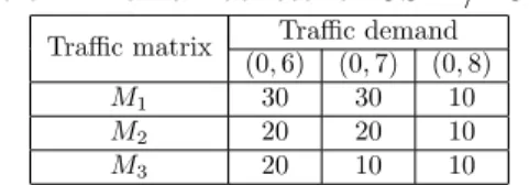
Table 1: Traffic matrices for OSPF/ECMP

Traffic matrix Traffic demand (0, 6) (0, 7) (0, 8)

M1 30 30 10

M2 20 20 10

M3 20 10 10

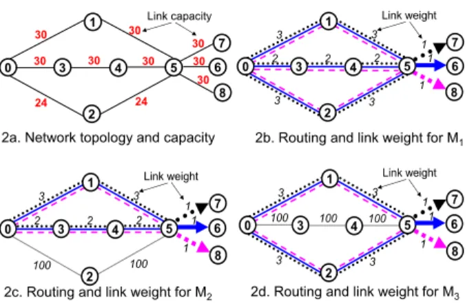
To better explain, we consider an example of a network topology with ca-pacity on links as shown in Fig. 2a. There are 3 traffic demands and we collect their values at 3 different periods, leading to 3 traffic matrices M1, M2 and

M3(Table 1). The routing solutions in Fig. 2 follow OSPF/ECMP (Equal-cost

multi-path) policy: a traffic demand flowing through a node i is equally split among all the interfaces connected to i which belong to at least one shortest path toward the considered destination. As shown in Fig. 2b, the three traf-fic demands are split among 3 different paths from 0 to 5, each path carries (30 + 30 + 10)/3 = 70/3 < 24. So, this routing is feasible but zero link can sleep. When traffic decreases, we can have better solutions. For example, 2 and 3 links are put in sleep mode for M2(Fig. 2c) and M3(Fig. 2d), respectively. The

2 0 1 8 7 6 5 4 3 30 30 30 30 30 24 24 30 30 30 Link capacity

2a. Network topology and capacity

2 0 1 5 4 3 3 2 Link weight 3 3 3 2 2 1 1 1 8 7 6 2 0 1 5 4 3 3 2 Link weight 3 100 100 2 2 1 1 1 8 7 6 2 0 1 5 4 3 3 100 Link weight 3 3 3 100 100 1 1 1 8 7 6

2c. Routing and link weight for M2 2d. Routing and link weight for M3

2b. Routing and link weight for M₁

Figure 2: Example of OSPF/ECMP for EAR

problem of optimizing the OSPF weight setting is known to be NP-hard, exact formulation and heuristic algorithm have been proposed in literature [21, 24].

2.2.1. Mixed integer linear program (MILP)

The MILP for the optimal OSPF weight setting problem was proposed in [11]. In this section, we reformulate the MILP to fit with our robust model (Section 2.3). The MILP uses the notations detailed on Table 2.

min X (u,v)∈E xuv (1) s.t. X v∈N (u) ¡ fvust − fuvst ¢ =      −1 if u = s, 1 if u = t, 0 else ∀u ∈ V, (s, t) ∈ D (2) X (s,t)∈D Dst_(fst uv+ fvust) ≤ µCuvxuv ∀(u, v) ∈ E (3) 0 ≤ zst u − fuvst ≤ 1 − kuvt ∀(s, t) ∈ D; (u, v) ∈ E (4) fst uv− ktuv≤ 0 ∀(s, t) ∈ D; (u, v) ∈ E (5) 1 − kt uv≤ rtv+ wuv− rut ≤ (1 − ktuv)M ∀t ∈ Dt; (u, v) ∈ E (6) kt uv− xuv≤ 0 ∀t ∈ Dt; (u, v) ∈ E (7) wuv≥ (1 − xuv)wmax ∀(u, v) ∈ E (8) xuv+ wuv≤ wmax ∀(u, v) ∈ E (9) 1 ≤ wuv ≤ wmax ∀(u, v) ∈ E (10) xuv, kuvt ∈ {0, 1}; fuvst, zust∈ [0, 1]; rtu≥ 0 (11)

Table 2: Notations

wmax the maximum value of a link weight.

M a large enough constant. It can be set M = 2wmax.

D a set of all traffic demands to be routed.

Dt a set containing all destination nodes.

Dst_{∈ D demand of the traffic flow from s to t.}

Cuv capacity of a link (u, v).

µ ∈ (0, 1] maximum link utilization that can be tolerated. It is normally set to a small value, e.g. µ = 0.5.

N (u) the set of neighbors of u in the network graph G.

kt

uv binary variable to determine if the link (u, v) belongs to one of the shortest paths from node u to node t.

zst

u variable to represent fraction of the flow (s, t) to be routed on outgoing node u using ECMP.

rt

u cost of the shortest path from u to t.

xuv binary variable to indicate if the link (u, v) is active or not.

fst

uv a flow (s, t) that is routed on the link (u, v).

The objective function (1) minimizes the power consumption of the network represented by the number of active links. Constraints (2) establish the clas-sical flow conservation constraints. We consider an undirected link capacity model [25] in which the capacity of a link is shared between the traffic in both directions. Constraints (3) limit the available capacity of a link (where µ

de-notes the maximum link utilization). The binary variable kt

uv = 1 if and only

if the link (u, v) belongs to one of the shortest paths from node u to node t.

Constraints (4) are for ECMP routing. It makes sure that if kt

uv = 1 then the

flow fst

vu destined to node t is equal to zstu, which is the common value of the flow assigned to all links outgoing from u and belonging to one of the shortest paths from u to t. Constraints (5) force fst

uv = 0 for all links (u, v) that do not belong to a shortest path to node t. The variable rt

u represents the cost of the shortest path from u to t. Constraints (6) compute the weight of link (u, v) if it belongs to the shortest path from u to t. Constraints (7) force link (u, v) to be on if it belongs to the shortest path from u to t. Note that, we do not force

xuv = 0 when ktuv = 0 because if (u, v) belongs another shortest path to t1 (in this case kt1

uv = 1 and xuv should be equal to 1). Constraints (8)-(10) guarantee that if a link weight is equal to wmax, then this link should be put into sleep mode.

2.2.2. Heuristic algorithm

Finding the optimal OSPF weight setting that deals with energy saving and/or traffic engineering issues is very challenging. We found in literature many works trying to solve this problem using heuristic approaches. For example, the authors in [24, 11] have proposed to use local search by iteratively modifying the OSPF weights so as to achieve the objective. The authors in [12] have

used genetic algorithms to find the link weights for the joint-optimization of load-balancing and energy efficiency. As the traffic matrices are considered independently, these algorithms can find different sets of link weights in the optimization process for each traffic matrix. We call these methods as freely

changed weight setting.

2.3. Γ-robust network design

Over the past years, robust optimization has been established as a special branch of mathematical optimization allowing to handle uncertain data [26]. A specialization of robust optimization, which is particularly attractive by its computational tractability, is the so-called Γ-robustness concept introduced by Bertsimas and Sim [27]. As observed in real traffic traces, only few of the de-mands are simultaneously at their peaks at a given time [28, 29]. For instance, Fig. 3 shows real traffic traces of the three source-destination pairs: (a) Wash-ington D.C. - Los Angeles, (b) Seattle - Indianapolis, and (c) Seattle - Chicago in the US Abilene Internet2 network in intervals of 5 mins during the first 10 days of July 2004 [28]. We observe that there is no point that all the three demands are at the peak values at the same time. Thus, it confirms the as-sumption: it is unlikely that all the traffic demands assume their peak values simultaneously. Peak traffic Peak traffic Peak traffic (a) (b) (c)

Figure 3: Traffic demands in Abilene network [28]

Γ-robust network design allows to choose an integer parameter Γ ≥ 0 so that at most Γ traffic demands can be at their peak values simultaneously. Note that, the model only limits a number of traffic demands (but not exactly which ones) that can be at their peaks at the same time. Therefore, from a practical perspective, by varying the parameter Γ, different solutions can be obtained with different levels of robustness. This concept has already been applied to several network optimization problems [30, 31, 32].

To better explain, we consider an example in Fig. 1. Again, we use a grid 3 × 4, each link has a capacity 4 Gbps (Fig. 1). There are 3 traffic demands, each has a nominal and peak values (in Gbps) as shown in Table 3.

Table 3: Traffic demand variation

Demand (s, t) Nominal value Peak value

(0, 3) 1 4

(4, 7) 1 3

(8, 11) 1 2

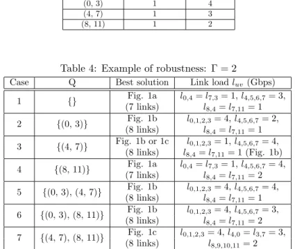
Table 4: Example of robustness: Γ = 2

Case Q Best solution Link load luv(Gbps)

1 {} Fig. 1a l0,4= l7,3= 1, l4,5,6,7= 3, (7 links) l8,4= l7,11= 1 2 {(0, 3)} Fig. 1b l0,1,2,3= 4, l4,5,6,7= 2, (8 links) l8,4= l7,11= 1 3 {(4, 7)} Fig. 1b or 1c l0,1,2,3= 1, l4,5,6,7= 4, (8 links) l8,4= l7,11= 1 (Fig. 1b) 4 {(8, 11)} Fig. 1a l0,4= l7,3= 1, l4,5,6,7= 4, (7 links) l8,4= l7,11= 2 5 {(0, 3), (4, 7)} Fig. 1b l0,1,2,3= 4, l4,5,6,7= 4, (8 links) l8,4= l7,11= 1 6 {(0, 3), (8, 11)} Fig. 1b l0,1,2,3= 4, l4,5,6,7= 3, (8 links) l8,4= l7,11= 2 7 {(4, 7), (8, 11)} Fig. 1c l0,1,2,3= 4, l4,0= l3,7= 3, (8 links) l8,9,10,11= 2

As an example, assume that Γ = 2, meaning that zero, one or two traffic demands can be at their peak values simultaneously. This leads to a combination of seven possibilities that are shown in Table 4. The set Q includes these seven cases.

It is easy to see that in Case 1, all traffic demands are at nominal values, hence as EAR, Fig. 1a is the best solution with only 7 active links. In Case 2, when (0, 3) is at peak (4 Gbps), solutions in Fig. 1b and Fig. 1d are feasible. However, Fig. 1b is the best solution since only 8 active links are used. Similarly, in Case 7, solutions in Fig. 1c and Fig. 1d are feasible and Fig. 1c is the best one. In summary, Table 4 shows a set of possible traffic realizations and the corresponding best solution when Γ = 2. However, since we just limit the number demands (but not any specific demands) to be deviated, a feasible solution should be the one that satisfies all the seven cases. Therefore, Fig. 1d is the only feasible solution for Γ = 2. It is also easy to check that, if we limit Γ = 1 (less robust), Fig. 1b is the best solution. From these examples, we can observe that, depending on the desired robustness of a network, a single routing solution can be feasible for many traffic matrices.

In this paper, our goal is to avoid weight changes as much as possible be-tween multi-period traffic matrices while minimizing energy consumption for the

networks. The main contributions are presented in Section 3, where we propose two methods to stabilize the OSPF weight setting (called stable weight setting and Γ-robust approach). To better assess the algorithm performance in terms of energy saving, we have implemented a simple freely changed weight setting algorithm (in Section 3.1.3) to compare with the stable weight setting and the Γ-robust approach.

3. Optimizing OSPF weight setting in multi-period traffic matrices

3.1. Stable weight setting

In this approach, multi-period traffic matrices are used to capture the daily traffic pattern. However, these traffic matrices are not considered independently. The idea is that, when changing from a more to a less traffic matrix (traffic load is reducing), we only consider to sleep unused links. In other words, any set of active links for low traffic is included in that of higher traffic. In addition, the weight setting of remaining links are unchanged. The reason is to limit changes in routing configuration and reduce network oscillations that affect QoS. As we add restrictions, stable weight setting has less potential in saving energy than the freely changed weight setting approach. For instance, as the example in Fig. 2, when traffic changes from M2 to M3, the stable weight setting can not have solution like Fig. 2d as both turning on and off links are necessary.

Since we try to stabilize the weight setting based on the previously used one, a question is how to find an initial weight setting that will be used for all the matrices of the multi-period traffic matrices. In fact, there are many ways to set link weights in practice. For instance, Cisco uses the inverse of link capacity; or more complicated load-balancing traffic engineering methods can be found in [21, 11, 12]. Actually, the initial set of weight has an impact on the energy saving in daily time. We can use the freely changed weight method to find a good configuration for a traffic matrix. However, this configuration may not be good for subsequent traffic matrices and how to find a good starter for the whole day traffic variation is beyond the scope of this paper. In this work, the network operators are free to choose their own weight setting. Anytime they would like to start energy saving mode, the stable algorithm can be applied directly using the current weight setting configuration as the initial one. We propose an exact formulation and heuristic algorithms for the stable weight setting method in the following sections.

3.1.1. Stable weight MILP

The inputs are network topology G = (V, E), traffic matrix D and a set of current link weights W . The output is a routing solution that minimizes the number of active links so that it satisfies constraints (2) - (11). Meanwhile, as the weight setting W should not be modified, following constraints should be added to the model (1) - (11):

wuv− wuv∗ ≥ (1 − xuv)(wmax− wuv∗ ) ∀(u, v) ∈ E (12)

w∗

We note w∗

uv as the current weight of the link (u, v). Constraints (12) - (13) are used to force the new link weight wuv to be equal to wuv∗ if the link (u, v) is still used in the new routing solution. Otherwise, wuvis set to wmax and the link (u, v) is put into sleep mode.

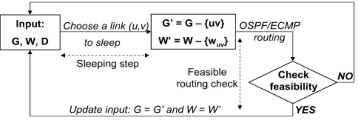
3.1.2. Stable Weight Heuristic

The stable weight setting problem is also very challenging for large networks. We propose in this section heuristic algorithms that can find feasible solution in an acceptable time. In brief, the heuristic algorithm includes sleeping step and

feasible routing check step (Fig. 4).

Check feasibility Input:

G, W, D

Choose a link (u,v) to sleep G’ = G – {uv} W’ = W – {w_uv} OSPF/ECMP routing NO Mark the link (u, v) as already checked link

YES

Update input: G = G’ and W = W’

Sleeping step

Feasible routing check

Figure 4: Heuristic diagram

There are many criteria to choose a link (u, v) to sleep (see in [11, 2]). In this paper, we propose to choose the min load link to sleep since this approach has been successfully applied in literature [11, 23, 10, 2, 33, 34]. After the sleeping

step, the feasible routing check step has inputs which are a subgraph G0_{, a subset}

of link weights W0 _{and the same traffic matrix D. We perform OSPF/ECMP}

routing for D on G0_{and check if some links are overloaded. If yes, the routing is} not feasible, we mark the slept link as checked and go back to the sleeping step to find another link to make sleeping (the checked links will not be chosen). If the routing is feasible, we update the inputs and go back to the sleeping step to continue. This procedure is repeated until all links on the network are checked. To deal with multi-period traffic matrices, we first sort the traffic matrices in non-increasing order of traffic load, that is from Dn to D1. The traffic load is computed as the sum of the volumes of all traffic demands in a traffic matrix.

Then, we run the MILP or heuristic algorithm for Dn to find a feasible network

configuration (link weight setting, set of links to sleep). Given this configuration as input, we find new feasible configuration for Dn−1in which we consider only to sleep links and the remaining links keep the same weight setting. As the traffic load of Dn is larger than that of Dn−1, it is highly probable to use more active links in Dn than in Dn−1. This process is repeated until we reach D1. Following the traffic variation of daily time, from a low to higher traffic matrices (e.g. Dito Di+1), we simply apply the configuration that has been found (from

Di+1 to Di). In this scenario, only slept links are woken up and the remaining links keep the same weight setting.

3.1.3. Freely changed weight heuristic

In order to compare the energy saving of the stable weight heuristic, we implemented a simple freely changed weight heuristic algorithm. Using the same diagram as in Fig. 4, at the feasible routing check step, we follow the idea of local search used in [24]. If the routing is infeasible, instead of marking the link as “checked” (impossible to sleep), we repeat the local search step, trying to find another feasible weight setting. The main idea is that: in each iteration, we increase the weights of the overloaded links to redirect traffic to other links, hoping that a new feasible routing solution can be found. Depending on the execution time of the algorithm, we can define a maximum number of loops for the local search. If there is still no feasible solution at the end of the iteration, we mark that link as “checked”, then the algorithm repeats the sleeping step described in Fig. 4 with another chosen link.

3.2. Γ-robust approach: one network configuration for all

We propose in this sub-section a method to find a single nework configuration with a set of active links and weight setting that is feasible for all the considered traffic matrices.

3.2.1. Robust MILP

Assume that each traffic demand has a nominal Dst and a deviated value

b

Dst _{so as the peak value is (D}st_{+ bD}st_{). Given a parameter 0 ≤ Γ ≤ |D|, the} robust model tries to find a feasible routing at minimal energy costs, while the link capacity constraints are satisfied if at most Γ traffic pairs simultaneously

deviate from their nominal values Dst. Note that Γ = |D| amounts to

worst-case optimization where all demands are at peak values. The straightforward robust capacity constraint for a given Γ and an edge e ∈ E is:

X (s,t)∈D Dstfst e + max_Q⊆D |Q|≤Γ n X (s,t)∈Q b Dst_fst e o ≤ µCexe ∀e ∈ E (14) where fst

e = fuvst + fvust; Q is a subset containing demands that can be at peaks at the same time. The constraints (14) is non-linear since it contains the max notation. A trivial way to make it linear is to explicitly write down all the possibilities of the constraints, that is:

X (s,t)∈D Dstfst e + X (s,t)∈Qi b Dst_fst e ≤ µCexe ∀Qi⊆ D; |Qi| ≤ Γ; e ∈ E (140)

Obviously, the constraints (140_{) is a combination of all possibilities of a} subset Qiwhich has the size |Qi| ≤ Γ. Therefore, it is impractical to put all the constraints into the MILP model at one time when the set of demand D is large. To overcome this problem, we apply the method Γ-robustness (introduced by Bertsimas and Sim [27]). The main idea of this method is to use LP duality to make a compact formulation, so that it is possible to solve the MILP. We present step-by-step the procedure to form the compact formulation as follows.

Assume that we know the value of fst

e (then they are constants), the

maxi-mum part of (14) can be computed by the following ILP:

β(f, Γ) := max X (s,t)∈D b Dst_fst e yest (15) s.t. X (s,t)∈D yst e ≤ Γ [πe] (16) yst e ∈ {0, 1} [ρste] (17)

where the primal binary variables yst

e denote whether or not fest is part

of the subset Q ⊆ D. As proposed by Bertsimas and Sim, we employ LP duality with the dual variables πe and ρste, which correspond to the constraints P

(s,t)∈Dyest ≤ Γ and yest ≤ 1, respectively. The LP duality for β(g, Γ) is as

follows: β(g, Γ) := min ³ Γπe+ X (s,t)∈D ρst e ´ (18) s.t. πe+ ρste ≥ bDstfest ∀(s, t) ∈ D (19) ρst e, πe≥ 0 ∀(s, t) ∈ D (20)

Since the constraints (18)–(20) are linear. A compact reformulation can be obtained by embedding them into (1)–(13). As a result, the robust stable weight setting can be compactly formulated as (1)–(2), (4)–(13) and replace (3) by:

X (s,t)∈D (Dstfest+ ρste) + Γπe≤ µxeCe ∀e ∈ E (21) πe+ ρste ≥ bDstfest ∀(s, t) ∈ D; ∀e ∈ E (22) ρst e, πe≥ 0 ∀(s, t) ∈ D; ∀e ∈ E (23)

3.2.2. Robust heuristic algorithm

The main idea of the heuristic algorithm is similar to the diagram in Fig. 4. However, is is difficult to check routing feasibility since we do not know explicitly which traffic demands are at peak values. To deal with this problem, we use the ILP constraints (21)–(23) for the feasible routing check step as they represent the robust capacity constraints. In details, we consider a simplified MILP of the

robust weight setting in which we only keep constraints (11) (remove variables kt uv, zstu, rut), and (21)–(23): X (s,t)∈D (Dstfst e + ρste) + Γπe≤ µxeCe ∀e ∈ E πe+ ρste ≥ bDstfest ∀(s, t) ∈ D; ∀e ∈ E ρst e, πe≥ 0; xe∈ {0, 1}; fest∈ [0, 1] ∀(s, t) ∈ D; ∀e ∈ E

The OSPF/ECMP routing on G0 _{with a set of link weight W}0 _implicitly satisfies the flow conservation constraint. In addition, we have in hand a set

of link weight W0_{, therefore all the constraints (2) – (10) are not needed in}

the simplified ILP. When performing OSPF/ECMP routing for the subgraph

G0 _{(after the sleeping step), we can get all the values of f}st

e and xe (xe = 0

if fst

e = 0 ∀(s, t) ∈ D, otherwise xe = 1). Given them as the inputs, the

variables xeand festin the simplified MILP are now fixed, only ρste and πeremain variables. Since the simplified MILP is used only to verify routing solution, we ignore the objective function. To check routing feasibility, we run the simplified MILP with inputs: G0_{, D, Γ, f}st

e and xe, if a feasible solution is returned, it means that the routing solution satisfies the robust capacity constraints. Then, we go back to the sleeping step and continue the algorithm as in Fig. 4. 4. Computational evaluation

We solved the MILP models with IBM CPLEX 12.4 solver. All computations were carried out on a 2.7 Ghz Intel Core i7 with 8 GB RAM. We consider real-life traffic traces collected from the SNDlib [35]: the U.S. Internet2 Network (Abilene) (|V | = 12, |E| = 15, |D| = 130), the Geant network (|V | = 22, |E| = 36, |D| = 387) and the Germany50 (|V | = 50, |E| = 88, |D| = 1595).

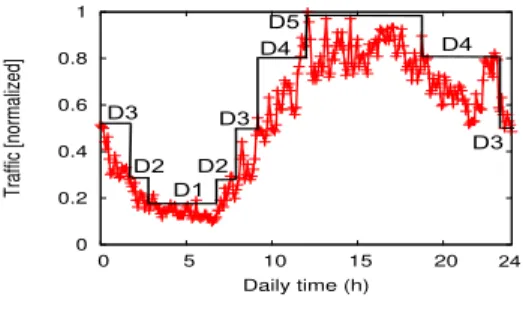
0 0.2 0.4 0.6 0.8 1 0 5 10 15 20 Traffic [normalized] Daily time (h) 24 D1 D2 D3 D2 D4 D4 D5 D3 D3

Figure 5: Daily traffic

In our test instances, five traffic matrices (D1 − D5) are used to represent daily traffic pattern (Fig. 5). From the SNDlib, we collect the mean and max traffic matrices (all traffic demands are at their mean and maximum values). Since traffic load is low, the mean traffic matrix is referred D1. To achieve a network with high link utilization, we scale the max traffic matrix with a factor of 1.3, 1.5, 1.8 and 2.0, in order to form D2 − D5, respectively. As a result, we represent D5 as the worst case scenario of highest traffic load. It is noted that, in reality, even at peak hour, not all the traffic demands are at their maximum values simultaneously as the case D5. The simulation results in this paper are based on the shape of the scaled traffic matrices D1 − D5. The results might be different if traffic demands vary more independently. In all test cases, as an approach of traffic engineering, we use a local search heuristic to find a set of link weights that minimize the maximum link load [24] for the traffic matrix D5. This weight setting is used as the initial one in the stable weight approaches.

4.1. Computation time

Table 5: Abilene network - optimal solutions Execution time (s)

D1 D2 D3 D4 D5

Stable weight MILP ≤ 5 ≤ 5 ≤ 5 ≤ 5 ≤ 5

Robust MILP 90

Freely changed weight MILP 95 874 100 12900 20700

Table 6: Geant network - heuristic solutions

Execution time (s)

D1 D2 D3 D4 D5

Stable weight 139 140 160 182 256 Robust stable weight 283

Freely changed weight 62 157 1596 2115 3600

Table 7: Germany network - heuristic solutions Execution time (s)

D1 D2 D3 D4 D5

Stable weight 468 1586 1787 2108 3108

Robust stable weight 3090

Freely changed weight 1739 3600 3600 3600 3600

For Abilene network, we can find optimal solution using the MILP for the three methods (stable, robust and freely changed weight). For larger network (e.g. Geant, Germany50), it is not possible to find even a feasible solution within 2 hours using the MILP, thus only the heuristic algorithms are used to find solutions for these large networks. The execution time of the freely changed

weight heuristic is limited to one hour by varying the number of loops in the

local search. For the robust stable weight, we run with different values of Γ and get an average running time.

It is clear that the stable weight and robust methods win a lot in running time. Indeed, these methods are based on an initial weight setting with a limited number of changes. Note that, we also use an initial weight setting for the robust case to limit network reconfiguration when changing from the normal (currently used) mode to the energy-aware mode. Thus, solution search space is small and optimal solutions can be found quite fast. Similar observation can be found for the heuristic approaches (Tables 6 and 7): the stable weight and robust methods take less than 1 hour for all test cases, meanwhile the execution time of the freely

changed weight reaches the time limit (set to 1 hour).

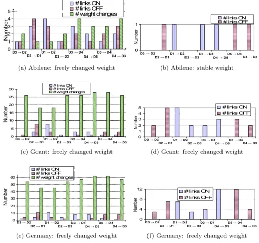
4.2. Stability of routing solutions

Fig. 6 shows changes in routing when shifting between periods of traffic during daily time. For the three tested networks, the stable weight approach always outperforms the freely changed weight. The former approach only allows

0 1 2 3 4 5 6 1 2 3 4 5 6 7 8 # links ON # links OFF # weight changes N u m b e r D1 → D2 D2 → D3 D3 → D4 D4 → D5 D5 → D4 D4 → D3 D2 → D1 D3 → D2

(a) Abilene: freely changed weight

0 1 1 2 3 4 5 6 7 8 # links ON # links OFF N u m b e r D1 → D2 D2 → D3 D3 → D4 D4 → D5 D5 → D4 D4 → D3 D2 → D1 D3 → D2

(b) Abilene: stable weight

0 5 10 15 20 25 30 1 2 3 4 5 6 7 8 # links ON # links OFF # weight changes N um be r D1 → D2 D2 → D3 D3 → D4 D4 → D5 D5 → D4 D4 → D3 D2 → D1 D3 → D2

(c) Geant: freely changed weight

0 1 2 3 4 5 1 2 3 4 5 6 7 8 # links ON # links OFF N u m b e r D1 → D2 D2 → D3 D3 → D4 D4 → D5 D5 → D4 D4 → D3 D2 → D1 D3 → D2

(d) Geant: freely changed weight

0 10 20 30 40 50 60 70 1 2 3 4 5 6 7 8 # links ON # links OFF # weight changes N u m b e r D1 → D2 D2 → D3 D3 → D4 D4 → D5 D5 → D4 D4 → D3 D2 → D1 D3 → D2

(e) Germany: freely changed weight

0 4 8 12 1 2 3 4 5 6 7 8 # links ON # links OFF N u m b e r D1 → D2 D2 → D3 D3 → D4 D4 → D5 D5 → D4 D4 → D3 D2 → D1 D3 → D2

(f) Germany: freely changed weight

Figure 6: Changes in freely changed weight vs. stable weight methods to sleep links (resp. only wake up links) when changing from a high traffic matrix to a lower one (resp. from a low to a higher traffic matrix). However, for freely changed weight, there is no restriction, link can be turned on and off and also the weight setting of remaining links can be changed. For instance, in Abilene network, from D3 to D2, even the energy saving (and the number of active links) is unchanged, the solution allows one link to turn off, one link to turn on and two active links change their weights. Similar observation can be found for Geant and Germany networks (Fig. 6c - Fig. 6f). The larger the network we consider, the more chaos we introduce as more changes happen between multi-period traffic matrices.

4.3. Energy saving in daily time

4.3.1. Stable weight vs. freely changed weight

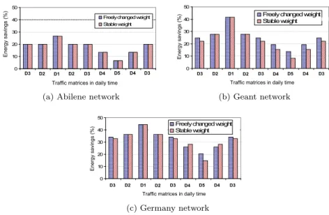
We show in Fig. 7 the energy saving of the three networks with traffic ma-trices in daily time. The energy saving is computed in comparison with the

0 10 20 30 40 50 1 2 3 4 5 6 7 8 9

Freely changed weight Stable weight E n e rg y sa vi n g s (% )

Traffic matrices in daily time

D3 D2 D1 D2 D3 D4 D5 D4 D3

(a) Abilene network

0 10 20 30 40 50 1 2 3 4 5 6 7 8 9

Freely changed weight Stable weight E n e rg y sa vi n g s (% )

Traffic matrices in daily time

D3 D2 D1 D2 D3 D4 D5 D4 D3 (b) Geant network 0 10 20 30 40 50 1 2 3 4 5 6 7 8 9

Freely changed weight Stable weight E n e rg y sa vi n g s (% )

Traffic matrices in daily time

D3 D2 D1 D2 D3 D4 D5 D4 D3

(c) Germany network

Figure 7: Energy saving in multi-period traffic matrices

case when all links on the networks are active. It is clear that energy saving is high when traffic load is low since more links can be put into sleep mode to save energy. To compare between stable weight and freely changed weight approaches, the latter one can save more energy because it is flexible to change the weight setting. This can be observed in D3, D4, D5 in Fig. 7b and D3, D5 in Fig. 7c. Abilene network is small and only a few links (from 1 to 4 links) can sleep, thus the solutions between the two methods are similar. It is noted that, in D4 (Fig. 7c), stable weight method even has better result. Indeed, we limit the number of loops so that the heuristic algorithm is finished after one hour. Thus, the freely changed weight heuristic may stop before finding a better solution than the stable weight approach. This can happen for large network is large, where the algorithm does several loops to find a good solution.

4.3.2. Robust vs. stable weight approaches

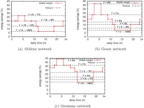
Fig. 8 shows energy saving of the stable weight setting vs. the Γ−robustness (with different value of Γ) in daily time traffic variation. We exploit the robust-ness to obtain a single on-off pattern for the whole day. Each dash line of the robust method corresponds to a Γ value which is applied for the whole day. For instance, in Abilene network (Fig. 8a), when Γ is less than 7%, we can find a single on-off feasible configuration which can save around 27% of energy for the whole day. Simulation results also confirm that the higher Γ is, the more robust, but the less power savings we achieve. Note that, when Γ = 100%, the robust model becomes the worst case of the deterministic - the case with D5 (all traffic demands are at their peak values). In all the three networks, the solutions do

0 5 10 15 20 25 30 35 40 45 0 5 10 15 20 energy savings (%) daily time (h) a Robust 24 Stable weight

(a) Abilene network

0 5 10 15 20 25 30 35 40 45 0 5 10 15 20 energy savings (%) daily time (h) a Robust 24 Stable weight (b) Geant network 0 5 10 15 20 25 30 35 40 45 0 5 10 15 20 energy savings (%) daily time (h) a Robust 24 Stable weight (c) Germany network

Figure 8: Robust weight vs. stable weight

not change when Γ is large enough (e.g. Γ = 14% for Abilene network). It is because in real traffic, only a small fraction of the demands dominates the others in volume. Therefore when the values of Γ cover all of these dominating demands, increasing Γ does not affect the routing solution and the percentage of energy saving remains the same. To give a visualized comparison, we also draw energy saving of the stable weight method in daily time. For instance, from Fig. 8a, if Γ = 9%, it is possible to have only one weight setting that gives fea-sible routing if at most 9% of traffic demands are at their peaks simultaneously. Moreover, this single weight setting allows to save the same amount of energy as the stable weight method for D2 or D3 matrices. Similar observations can be found for Geant (Fig. 8b) and Germany network (Fig. 8c). However, Geant and Germany networks are more sensitive with traffic variation, and significant energy saving is found only with small Γ.

4.4. Traffic load

4.4.1. Stable weight vs. freely changed weight

In the simulation, we set the maximum link utilization µ = 100%. Intuitively, EAR would affect the utilization of links as fewer links are used to carry traffic. In this subsection, we evaluate the impact of EAR on link utilization. We draw the cumulative distribution function (CDF) of link load of Abilene, Geant and Germany networks in Fig. 9. To test the worst case scenario, we use the

0 20 40 60 80 100 0 20 40 60 80 100 Fraction of links (%) Link load (%) Optimal freely changed weight

Optimal stable weight

(a) Abilene network

0 20 40 60 80 100 0 20 40 60 80 100 Fraction of links (%) Link load (%) Freely changed weight

Stable weight (b) Geant network 0 20 40 60 80 100 0 20 40 60 80 100 Fraction of links (%) Link load (%) Freely changed weight

Stable weight

(c) Germany network

Figure 9: CDF traffic load - freely changed weight vs. stable weight highest traffic matrix (D5). Since we guarantee capacity constraints, no link is overloaded. Our goal is not load balancing, thus we do not have an explicit comparison between the freely changed weight and the stable weight methods. However, from Fig. 9a, the stable weight method is slightly better, e.g. 60% of links have link utilization less than 80%, meanwhile it is only 40% of links for the freely changed weight method. This can be explained as the stable weight method uses an initial load-balancing link weight which is the one that minimizes the maximum link load.

4.4.2. Robust approach

For each value of Γ, we find a link weight setting that satisfies the capacity constraint if at most Γ demands are at peaks at the same time. However, we would like to test what will happen if we use a single robust network configu-ration while traffic is variated in daily time. Fig. 10 shows the maximum link utilization over all active links in the network for different values of Γ. Obvi-ously, if we use Γ = 100%, we can find a single network configuration that is feasible (no overloaded link) for all-day traffic variation. However, the price of this solution is too expensive: e.g. only 6% of energy can be saved for the Abi-lene network (like the case D5). However we observe that, even with Γ = 1%, the maximum link utilization of the three networks is less than 200%. It means that if we carefully set the value of µ in the capacity constraints (e.g. µ = 50%), then the robust solution with Γ = 1% can be feasible for all-day traffic variation.

0 50 100 150 200 0 5 10 15 20 Link utilization (%) Daily time (h) Gamma = 7% - MLU (%) Gamma = 13% - MLU (%) Gamma = 100% - MLU (%)

(a) Abilene network

0 50 100 150 200 0 5 10 15 20 Link utilization (%) Daily time (h) Gamma = 1% - MLU (%) Gamma = 6% - MLU (%) Gamma = 100% - MLU (%) (b) Geant network 0 50 100 150 200 0 5 10 15 20 Link utilization (%) Daily time (h) Gamma = 1% - MLU (%) Gamma = 2% - MLU (%) Gamma = 100% - MLU (%) (c) Germany network

Figure 10: Maximum link utilization (MLU) of robust solution in daily traffic If one network configuration fits for all is too greedy, a few robust configurations are also enough for the whole day traffic. For instance, in Abilene network, we can use 4 periods: 2h − 9h (Γ = 7%); 9h − 11h (Γ = 13%); 11h − 19h (Γ = 100% - D5 traffic matrix) and 19h − 2h (Γ = 13%). However, it may save less energy with respect to the stable weight approach as daily traffic is divided into 9 pe-riods and we assume that traffic matrix is accurately collected for each period. 5. Conclusion

To the best of our knowledge, this is the first work considering the stability of routing solution in energy-aware traffic engineering using OSPF protocol. We argue that, in addition to capacity constraints, the requirements on routing stability also play an important role in QoS. Moreover, using real traffic traces in the simulations, we show that our stable weight and robust methods are able to save a significant amount of energy. For future work, we will focus on how to find a good initial weight setting.

Acknowledgements

This work was partly funded by the French Government (National Research Agency, ANR) through the Investments for the Future Program reference ANR-11-LABX-0031-01, ANR project Stint under reference ANR-13-BS02-0007, the

CNRS-FUNCAP project GAIATO, the associated Inria team AlDyNet and the project ECOS-Sud Chile.

References

[1] “An inefficient Truth”, http://globalactionplan.org.uk (2007).

[2] L. Chiaraviglio, M. Mellia, F. Neri, “Minimizing ISP Network Energy Cost: Formulation and Solutions”, IEEE/ACM Transaction in Networking 20 (2011) 463 – 476.

[3] R. Bolla, F. Davoli, R. Bruschi, K. Christensen, F. Cucchietti, S. Singh, “The Potential Impact of Green Technologies in Next-generation Wireline Networks: Is There Room for Energy Saving Optimization?”, IEEE Com-munications Magazine 49 (2011) 80 – 86.

[4] C. Lange, “Energy-related aspects in backbone networks”, in: 35th Euro-pean Conference on Optical Communication, 2009.

[5] R. Bolla, R. Bruschi, F. Davoli, F. Cucchietti, “Energy Efficiency in the Future Internet: A Survey of Existing Approaches and Trends in Energy-Aware Fixed Network Infrastructures”, IEEE Communication Surveys and Tutorials 13 (2011) 223 – 244.

[6] A. P. Bianzino, C. Chaudet, D. Rossi, J. Rougier, “A Survey of Green Net-working Research”, IEEE Communication Surveys and Tutorials 14 (2012) 3 – 20.

[7] P. Mahadevan, P. Sharma, S. Banerjee, “A Power Benchmarking Frame-work for NetFrame-work Devices”, in: IFIP NETWORKING, 2009, pp. 795–808. [8] M. Gupta, S. Singh, “Greening of the Internet”, in: ACM SIGCOMM,

2003, pp. 19–26.

[9] L. Chiaraviglio, A. Cianfrani, E. L. Rouzic, M. Polverini, “Sleep Modes Ef-fectiveness in Backbone Networks with Limited Configurations”, Computer Networks 57 (2013) 2931–2948.

[10] F. Giroire, J. Moulierac, T. K. Phan, F. Roudaut, “Minimization of Net-work Power Consumption with Redundancy Elimination”, in: IFIP NET-WORKING, 2012, pp. 247–258.

[11] E. Amaldi, A. Capone, L. G. Gianoli, “Energy-aware IP Traffic Engineering with Shortest Path Routing”, Computer Networks 57 (2013) 1503–1517. [12] F. Francois, N. Wang, K. Moessner, S. Georgoulas, “Green IGP Link

Weights for Energy-efficiency and Load-balancing in IP Backbone Net-works”, in: IFIP NETWORKING, 2013, pp. 1–9.

[13] M. Shen, H. Liu, K. Xu, N. Wang, Y. Zhong, “Routing On Demand: To-ward the Energy-Aware Traffic Engineering with OSPF”, in: IFIP NET-WORKING, 2012, pp. 232–246.

[14] A. Capone, C. Cascone, L. G. Gianoli, B. Sans`o, “OSPF Optimization via Dynamic Network Management for Green IP Networks”, in: Sustainable Internet and ICT for Sustainability (SustainIT), 2013, pp. 1–9.

[15] S. S. W. Lee, P. Tseng, A. Chen, “Link Weight Assignment and Loop-free Routing Table Update for Link State Routing Protocols in Energy-aware Internet”, Future Generation Computer Systems 28 (2012) 437–445. [16] A. Cianfrani, V. Eramo, M. Listanti, M. Polverini, A. V. Vasilakos, “An

OSPF-Integrated Routing Strategy for QoS-Aware Energy Saving in IP Backbone Networks”, IEEE Transactions on Network and Service Manage-ment 9 (2012) 254 – 267.

[17] A. Cianfrani, V. Eramo, M. Listanti, M. Marazza, E. Vittorini, “An En-ergy Saving Routing Algorithm for a Green OSPF Protocol”, in: IEEE INFOCOM Workshop, 2010, pp. 1–5.

[18] A. Cianfrani, V. Eramo, M. Listanti, M. Polverini, “An OSPF Enhance-ment for Energy Saving in IP Networks”, in: IEEE INFOCOM Workshop, 2011, pp. 325–330.

[19] E. Amaldi, A. Capone, L. G. Gianoli, L. Mascetti, “Energy Management in IP Traffic Engineering with Shortest Path Routing”, in: IEEE WoWMoM, 2011, pp. 1–6.

[20] B. Addis, A. Capone, G. Carello, L. G. Gianoli, B. Sans`o, “Energy Man-agement Through Optimized Routing and Device Powering for Greener Communication Networks”, IEEE/ACM Transactions on Networking 22 (2014) 313 – 325.

[21] B. Fortz, M. Thorup, “Optimizing OSPF/IS-IS Weights in a Changing World”, IEEE Journal on Selected Areas in Comm. 20 (2002) 756–767. [22] A. Basu, J. Riecke, “Stability Issues in OSPF Routing”, in: ACM

SIG-COMM, Vol. 31, 2001, pp. 225–236.

[23] F. Giroire, D. Mazauric, J. Moulierac, B. Onfroy, “Minimizing Routing En-ergy Consumption: from Theoretical to Practical Results”, in: IEEE/ACM GreenCom, 2010, pp. 252–259.

[24] B. Fortz, M. Thorup, “Internet Traffic Engineering by Optimizing OSPF Weights”, in: IEEE INFOCOM, 2000, pp. 519–528.

[25] C. Raack, A. Koster, S. Orlowski, R. Wess¨aly, “On Cut-based Inequalities for Capacitated Network Design Polyhedra”, Networks 57 (2011) 141 – 156. [26] A. Ben-Tal, L. E. Ghaoui, A. Nemirovski, “Robust optimization”,

Prince-ton Series in Applied Mathematics, PrincePrince-ton University Press, 2009. [27] D. Bertsimas, M. Sim, “The Price of Robustness”, Operations Research 52

(2004) 35 – 53.

[28] A. Koster, M. Kutschka, C. Raack, “Robust Network Design: Formulation, Valid Inequalities, and Computations”, Networks 61 (2013) 128 – 149. [29] K. Zheng, X. Wang, L. Li, X. Wang, “Joint Power Optimization of Data

Center Network and Servers with Correlation Analysis”, in: IEEE INFO-COM, 2014, pp. 2598–2606.

[30] A. Koster, M. Kutschka, C. Raack, “On the Robustness of Optimal Network Designs”, in: IEEE ICC, 2011, pp. 1 – 5.

Optimization Approach for Energy-aware Routing in MPLS Networks”, in: IEEE ICNC, 2013, pp. 567–572.

[32] D. Coudert, A. Koster, T. K. Phan, M. Tieves, “Robust Redundancy Elimi-nation for Energy-aware Routing”, in: IEEE GreenCom, 2013, pp. 179–186. [33] F. Giroire, J. Moulierac, T. K. Phan, F. Roudaut, “Minimization of Net-work Power Consumption with Redundancy Elimination”, in: Computer Communications, 2014.

[34] F. Giroire, J. Moulierac, T. K. Phan, “Optimizing Rule Placement in Software-Defined Networks for Energy-aware Routing”, in: IEEE GLOBE-COM, 2014.