HAL Id: hal-00296146
https://hal.archives-ouvertes.fr/hal-00296146
Submitted on 14 Feb 2007
HAL is a multi-disciplinary open access
archive for the deposit and dissemination of
sci-entific research documents, whether they are
pub-lished or not. The documents may come from
teaching and research institutions in France or
abroad, or from public or private research centers.
L’archive ouverte pluridisciplinaire HAL, est
destinée au dépôt et à la diffusion de documents
scientifiques de niveau recherche, publiés ou non,
émanant des établissements d’enseignement et de
recherche français ou étrangers, des laboratoires
publics ou privés.
vertical dispersion for CO and SO2 in the Mexico City
Metropolitan Area using Solar FTIR and zenith sky UV
spectroscopy
B. de Foy, W. Lei, M. Zavala, R. Volkamer, J. Samuelsson, J. Mellqvist, B.
Galle, A.-P. Martínez, M. Grutter, A. Retama, et al.
To cite this version:
B. de Foy, W. Lei, M. Zavala, R. Volkamer, J. Samuelsson, et al.. Modelling constraints on the
emission inventory and on vertical dispersion for CO and SO2 in the Mexico City Metropolitan Area
using Solar FTIR and zenith sky UV spectroscopy. Atmospheric Chemistry and Physics, European
Geosciences Union, 2007, 7 (3), pp.781-801. �hal-00296146�
www.atmos-chem-phys.net/7/781/2007/ © Author(s) 2007. This work is licensed under a Creative Commons License.
Chemistry
and Physics
Modelling constraints on the emission inventory and on vertical
dispersion for CO and SO
2
in the Mexico City Metropolitan Area
using Solar FTIR and zenith sky UV spectroscopy
B. de Foy1,*, W. Lei2, M. Zavala2, R. Volkamer3, J. Samuelsson4, J. Mellqvist4, B. Galle4, A.-P. Mart´ınez5, M. Grutter6, A. Retama7, and L. T. Molina1,2
1Molina Center for Energy and the Environment, La Jolla, USA
2Department of Earth, Atmospheric and Planetary Sciences, Massachusetts Institute of Technology, USA 3Department of Chemistry and Biochemistry, University of California, San Diego, USA
4Department of Radio and Space Science, Chalmers University of Technology, Gothenburg, Sweden
5General Direction of the National Center for Environmental Research and Training (CENICA), National Institute of Ecology
(INE), Mexico
6Centro de Ciencias de la Atm´osfera, Universidad Nacional Aut´onoma de M´exico, Mexico 7Secretar´ıa del Medio Ambiente, Gobierno del Distrito Federal, Mexico
*now at: Saint Louis University, USA
Received: 19 June 2006 – Published in Atmos. Chem. Phys. Discuss.: 11 July 2006 Revised: 8 January 2007 – Accepted: 9 February 2007 – Published: 14 February 2007
Abstract. Emissions of air pollutants in and around urban
ar-eas lead to negative health impacts on the population. To es-timate these impacts, it is important to know the sources and transport mechanisms of the pollutants accurately. Mexico City has a large urban fleet in a topographically constrained basin leading to high levels of carbon monoxide (CO). Large point sources of sulfur dioxide (SO2) surrounding the basin
lead to episodes with high concentrations. An Eulerian grid model (CAMx) and a particle trajectory model (FLEXPART) are used to evaluate the estimates of CO and SO2in the
cur-rent emission inventory using mesoscale meteorological sim-ulations from MM5. Vertical column measurements of CO are used to constrain the total amount of emitted CO in the model and to identify the most appropriate vertical disper-sion scheme. Zenith sky UV spectroscopy is used to esti-mate the emissions of SO2from a large power plant and the
Popocat´epetl volcano. Results suggest that the models are able to identify correctly large point sources and that both the power plant and the volcano impact the MCMA. Mod-elled concentrations of CO based on the current emission in-ventory match observations suggesting that the current total emissions estimate is correct. Possible adjustments to the spatial and temporal distribution can be inferred from model results. Accurate source and dispersion modelling provides Correspondence to: B. de Foy
(bdefoy@mce2.org)
feedback for development of the emission inventory, verifica-tion of transport processes in air quality models and guidance for policy decisions.
1 Introduction
Detailed and accurate emission inventories are a cornerstone of effective air quality management programs. Public pol-icy choices can be evaluated with air quality models based on actual emissions and alternative scenarios in combination with accurate meteorological simulations. This paper makes use of novel measurement techniques to evaluate the carbon monoxide (CO) inventory for the Mexico City Metropolitan Area (MCMA) and to evaluate the potential impacts of large point sources of sulfur dioxide (SO2). Even though vertical
dispersion has a large impact on pollutant transport, it can be overlooked as a source of uncertainty. Pollution observa-tions and simulaobserva-tions are further used to evaluate alternative vertical dispersion schemes.
1.1 Mexico City Metropolitan Area
Megacities are home to a growing number of people and can suffer from high levels of air pollution (Molina and Molina, 2004; Molina et al., 2004). The MCMA is a megacity of
around 20 million people living in a basin 100 km in di-ameter at 2240 m altitude and 19◦N latitude. The basin is surrounded by high mountains on the west, south and east. There is intense solar radiation and high ozone levels most of the year. There has been extensive scientific study of the air quality in the MCMA, as reviewed in Molina and Molina (2002).
Nickerson et al. (1992) carried out aircraft profiles of ozone, SO2and particulate matter (PM) above Mexico City
in 1991, highlighting the importance of combustion sources for the basin air pollution. Williams et al. (1995) modelled air dispersion for the same episodes looking at the transport of contaminants towards the southwest of the basin and empha-sizing the need for improved accuracy of the emission inven-tory. Elliott et al. (1997) analysed the importance of liquefied petroleum gas (LPG) components in the urban air chemistry. By estimating CO residence times of approximately 2 days in the basin, estimates are made of the LPG venting to the regional environment.
Fast and Zhong (1998) developed a wind circulation model for the basin from data obtained during the IMADA cam-paign of 1997. This emphasized the importance of verti-cal mixing and mountain winds in the transport of the urban plume first towards the south and then back over the city to the north. Similar patterns are described in Jazcilevich et al. (2003) with evidence of direct convective transport from lay-ers aloft to the surface.
MCMA-2003 was a major field campaign that took place in April 2003. De Foy et al. (2005) reviewed wind circula-tion patterns in the basin and classified the meteorological conditions into 3 episode types. O3-South are days when ozone is high in the south and a weak late afternoon jet flow forms. O3-North days are when the ozone peak is in the north due to the combination of a strong jet and flow over the south and west edges of the basin. Cold Surge days are when cold northerlies sweep the basin atmosphere clean. These episodes were subsequently used to analyse the transport and basin venting (de Foy et al., 2006c) using a mesoscale meteo-rological model and Lagrangian particle model. Whereas El-liott et al. (1997) suggested residence times as long as 2 days, this found residence times frequently as low as 6 to 12 h in the basin and little carry-over from day to day. The present analysis is based on the meteorological simulations described in de Foy et al. (2006c), making use of the 3 episode types and the short residence times.
1.2 Emission inventory
Emission inventories can be derived using either the “top-down” method, where total fuel and energy consumption are used for a whole region to determine surface emissions or the “bottom-up” method, where estimates of vehicle miles travelled and residential, industrial and commercial energy use patterns are considered. The 2002 official emission in-ventory for the MCMA used in this study was derived by the
bottom-up method by the Comisi´on Ambiental Metropoli-tana (CAM) of the Mexican Federal District government (Comisi´on Ambiental Metropolitana, 2004). This contains annual totals for the criteria pollutants which need to be temporally and spatially distributed as well as speciated for VOCs (West et al., 2004).
Due to technology change, CO emissions have been de-creasing despite increases in vehicular traffic. Schifter et al. (2005) develop a top-down estimate of vehicular emissions by combining fuel use statistics with emission factors ob-tained from in-situ remote sensing experiments. This sug-gests that, if anything, the official inventory may overesti-mate CO emissions. Jiang et al. (2005) obtain emission fac-tors for the MCMA vehicle fleet by analysing data from the Aerodyne mobile laboratory (Kolb et al., 2004) for CO, black carbon, polycyclic aromatic hydrocarbons and other pollu-tants. For CO, a similar conclusion to Schifter et al. (2005) is drawn, that official inventory estimates are high but in gen-eral agreement. Zavala et al. (2006) analyse chase and fleet average mode data in detail, determining emission factors from individual vehicle plumes and obtaining emission es-timates for individual vehicle types. This provides valuable information on NOx, aldehydes, ammonia and certain VOC’s
which will be used to further refine the emission inventory and guide policy work. West et al. (2004) modelled the pho-tochemistry in the basin during the IMADA campaign us-ing the 1998 official inventory of the CAM, suggestus-ing that emissions of CO need to be scaled by a factor of 2 and that of volatile organic compounds (VOCs) by a factor of 3.
Olivier and Berdowski (2001) develop the EDGAR global emission inventory at a 1 degree resolution. For Mexico the emissions of the MCMA are about ten times larger than an-thropogenic sources outside of the basin. This means that within the accuracy of the present modelling work, regional emissions can be represented through appropriate settings of the boundary conditions.
On the regional scale, Kuhns et al. (2005) report on the development of an emission inventory for the northern part of Mexico as part of the BRAVO study. This includes the MCMA inventory but not the surrounding region. Also in-cluded are estimates of SO2emissions from the Popocat´epetl
volcano and the Tula industrial complex, two large point sources shown in Fig. 1. The Tula source consists of both a power plant and a refinery. The Popocat´epetl volcano is an active volcano forming the southeastern edge of the MCMA basin. It has been under continuous monitoring by the Centro Nacional de Prevenc´ıon de Desastres (CE-NAPRED). Kuhns et al. (2005) report SO2 emission
esti-mates made with a correlation spectrometer (COSPEC) as high as 18×106tonne/year but more typically around 1.1 to 1.8×10⁶tonne/year.
Raga et al. (1999) analysed SO2, CO and aerosol
mea-surements in the MCMA and suggested that increased sulfate aerosol production in the city could be due to volcanic emis-sions. Jimenez et al. (2004) report on a field study carried
out between Popocat´epetl and Puebla (to the east). Clear ev-idence was found of volcanic influence at the surface for 6 out of 17 days sampled.
Column measurements of CO can be used in conjunc-tion with dispersion models to constrain emission invento-ries. For example, Yurganov et al. (2004) obtain CO columns from Fourier Transform Infrared (FTIR) spectrometers. A box model and the 3-D global GEOS-CHEM model (Bey et al., 2001) are used to evaluate the emissions from boreal wild fires in August 1998. Yurganov et al. (2005) extend the analysis to 2002 and 2003. Strong correlations are found be-tween estimates from surface measurements and those from MOPITT CO columns.
1.3 Source identification
Blanchard (1999) reviews different methods for estimating the impacts of emission sources on air pollutant levels. These can be separated into data analysis methods and model-based methods. The latter includes forward and backward trajec-tory analyses as well as Eulerian dispersion models. Hopke (2003) reviews further developments of receptor models and back trajectory analyses. “Residence Time Analysis” and “Potential Source Contribution Function” are described and compared using case studies in the northeast of the U.S.
“Residence Time Analysis” was introduced by Ashbaugh et al. (1985). It is a 2-D gridded field that represents the probability that a randomly selected air parcel is to be found in a grid cell relative to the total time interval of the trajec-tory. Dividing the probability of a “dirty” air parcel being in a grid cell with the probability of any air parcel passing through that cell, one obtains the “Potential Source Contri-bution Function”. This normalised field will have high val-ues over regions of high emissions. The method was used to show that the dominant source of sulfur in the Grand Canyon national park was from southern California.
Sirois and Bottenheim (1995) define “Probability of Res-idence” by applying the Residence Time Analysis of Ash-baugh et al. (1985) to the trajectories associated with the highest and lowest 10% of air pollutant concentrations. A cluster analysis was then performed on all backward trajec-tories at the receptor site. Analysis of the pollution levels as-sociated with each cluster showed agreement with the “Prob-ability of Residence” method while providing additional in-formation about air mass movements. Vasconcelos et al. (1996a) apply the method of Ashbaugh et al. (1985) to field campaign data in the Grand Canyon, again identifying south-ern California as the main source region. The spatial resolu-tion of their results is analysed in Vasconcelos et al. (1996b). This suggested that the method has good resolution in source direction but significantly less in radial distance from the re-ceptor site. Long trajectories (5 days in this case) have higher uncertainties, but short trajectories (3 days) can miss distant sources and suggest spurious source regions near the recep-tor. 440 460 480 500 520 540 2100 2120 2140 2160 2180 2200 2220 VIF CENICA SATL POPO TULA MER PED AZC XAL TLI BC1 BC2 BC3 BC4 UTM East (km) UTM North (km) Ajusco Chalco Toluca Puebla Mexican Plateau
Fig. 1. Map of the MCMA showing the Tula industrial complex,
Popocat´epetl volcano, CENICA supersite, Santa Ana Tlacotenco (SATL) boundary site, SOF column measurement boundary sites and RAMA surface sites (crosses, see Fig. 11 for additional station names). Political border of the MCMA as of 2003 in pink, urban area in beige, terrain contour every 500 m.
Stohl (1998) reviews the applications and accuracy of tra-jectories. “Concentration Fields” are described as Residence Time Analysis multiplied by pollutant concentrations at the receptor site for each measurement time (Seibert et al., 1994). Lupu and Maenhaut (2002) show that the Potential Source Contribution Function and Concentration Field methods are in agreement over the identification of European emissions based on measurements at different peripheral sites. The bootstrap technique is used to estimate the statistical signif-icance of potential sources, and known emission sources are shown to be correctly identified.
Use of single trajectories does not account for the spread in possible source directions due to vertical and horizontal mixing. Jiang et al. (2003) calculate retro-plumes by running a dispersion model, CALPUFF, in reverse mode. This yields the equivalent of Concentration Fields that account for all the processes parameterised in CALPUFF, including dispersion and deposition. By replacing single trajectory analyses with a Lagrangian particle dispersion model, Stohl et al. (2002) account for both physical dispersion and numerical uncer-tainty in the trajectory locations.
1.4 Vertical dispersion
As the resolution of meteorological models increases both in the horizontal and in the vertical, the parameterisation of the
surface energy budget and that of the vertical mixing become more important in terms of simulation accuracy (Zhong and Fast, 2003). Nevertheless, Berg and Zhong (2005) found that despite the different boundary layer schemes in MM5 and the different levels of mixing they simulate, there is little gain in the overall accuracy of the forecasts due to their increased complexity. Air quality models usually include a choice of vertical dispersion schemes based on output from the meteo-rological models, for example the widely-used parameterisa-tion scheme of O’Brien (1970).
Evaluating vertical diffusion coefficients is difficult be-cause the numerical representation does not account for the complexity of the physical process and because the diffusion coefficients cannot be measured directly. Atmospheric con-centrations of radio-nucleides provides an indirect method of evaluating the dispersion. Vertical profiles of222Rn in the lower atmosphere have been used (Lee and Larsen, 1997), (Olivie et al., 2004).
For air quality models, the vertical dispersion has a di-rect impact on simulated surface concentrations. Nowacki et al. (1996) found excessive vertical mixing in the day time unstable boundary layer leading to errors in surface concen-trations. Improvements in the specification of the vertical diffusion coefficients were suggested but evaluation was lim-ited due to the lack of measurements of the vertical concen-tration profiles. Biswas and Rao (2001) report substantial differences between different models adding to uncertainties in ozone simulations and Roelofs et al. (2003) suggest that coarse vertical resolution may lead to excessive dispersion.
Brandt et al. (1998) analysed different vertical dispersion schemes and found that the simplest scheme of high vertical dispersion yielded the best results, suggesting that non-local dispersion is an important factor. Ulke and Andrade (2001) propose a new parameterisation which yields higher surface concentrations in the CIT model. They also highlight the problem of validating emissions inventories with surface data but no vertical profiles. Perez-Roa et al. (2006) use artificial neural networks to develop site-specific optimal estimates of vertical diffusion coefficients. They show improved surface concentrations of CO and particulate matter using the CAMx model, as well as possible adjustments to the emission inven-tory.
Jazcilevich et al. (2005) use vertical diffusion coefficients from the Burk-Thompson scheme in MM5 for their simula-tions of the MCMA. In contrast to West et al. (2004) who used the CIT coefficients, no adjustments factors are needed to the CO emission inventory. Although the 1994 official inventory is used rather than the 1998 one, this suggests that differences between models can impact the conclusions drawn about the inventory.
1.5 Outline
This paper makes use of Concentration Fields from back-ward trajectories and forback-ward Eulerian dispersion modelling
to analyse the emission inventory for CO and SO2. Column
measurements of CO are used as a constraint on the verti-cal dispersion scheme. SO2 emission fluxes are estimated
from large point sources so as to simulate their impact on the MCMA. Section 2 describes the models used and Sect. 3 the observations. The analysis of the emission inventory is split by pollutant: Sect. 4 looks at CO and Sect. 5 looks at SO2.
Each section is split into a first part using backward trajecto-ries, a second part using Eulerian modelling and a discussion section.
2 Model description
The Pennsylvania State University/National Center for At-mospheric Research Mesoscale Model (MM5, Grell et al., 1995) version 3.7.2 was used to generate the wind fields as described in de Foy et al. (2006b). This uses three nested grids with one-way nesting at resolutions of 36, 12 and 3 km, with 40×50, 55×64 and 61×61 grid cells for domains 1, 2 and 3, respectively, and are the same simulations used in de Foy et al. (2006a). The initial and boundary conditions were taken from the Global Forecast System (GFS) at a 3-h resolution. High resolution satellite remote sensing is used to initialise the land surface parameters for the NOAH land surface model, as described in de Foy et al. (2006b).
The emission inventory used for CO and SO2is based on
West et al. (2004) with updated totals from Comisi´on Am-biental Metropolitana (2004). The spatial pattern of the CO area sources is shown in Fig. 2a, and the point sources in Fig. 2c. The SO2emissions are shown in Figs. 2b and d. The
temporal profile of both CO and SO2is shown in Fig. 3. This
shows that the point sources are negligible for CO and small for SO2, although including the Tula industrial complex and
Popocat´epetl volcano would change this picture. There is a clear peak at the morning rush hour, sustained traffic through-out the day and reduced emissions at night.
Stochastic particle trajectories are calculated using FLEX-PART (Stohl et al., 2005), as described in de Foy et al. (2006c). Backward trajectories are calculated for specific fixed sites. For these cases, 100 particles per hour are re-leased between 0 and 50 m above ground and are traced back for 48 h. Forward trajectories are calculated with the CO spa-tial and temporal distribution described above to provide sim-ulated CO fields.
Residence Time Analysis was carried out using the parti-cle simulations following Ashbaugh et al. (1985). For a one hour release, all particle positions at every hour of the simula-tion are stored. A surface grid is applied over the simulasimula-tion domain, and all particle positions in each grid cell are totalled for the entire simulation. This gives “Residence Times”, the grid corresponds to a time exposure photograph of the parti-cle tracks, with values equivalent to the length of time spent in each cell by particles emitted.
0 2500 5000 7500 10000 12500 15000 17500 20000 22500 25000 g/s 440 460 480 500 520 540 2100 2120 2140 2160 2180 2200 2220 UTM East (km) UTM North (km) CO Area Sources 0 20 40 60 80 100 120 140 160 180 200 g/s 440 460 480 500 520 540 2100 2120 2140 2160 2180 2200 2220 UTM East (km) UTM North (km) SO 2 Area Sources 0 100 200 300 400 500 600 700 800 900 1000 g/s 440 460 480 500 520 540 2100 2120 2140 2160 2180 2200 2220 UTM East (km) UTM North (km) CO Point Sources 0 50 100 150 200 250 300 350 400 450 500 g/s 440 460 480 500 520 540 2100 2120 2140 2160 2180 2200 2220 POPO TULA UTM East (km) UTM North (km) SO 2 Point Sources
Fig. 2. Daily emission totals for CO (left) and SO2(right) from area (top) and point sources (bottom). Point sources are summed to the same grid as the area sources for ease of comparison. Note different scale for each plot. Location of Tula and Popocat´epetl shown by the star (not colour coded).
The Residence Times can be summed for hourly releases during the whole campaign to identify preferred transport di-rections. In order to identify possible source regions, Con-centration Fields were calculated. To derive these, Residence Times from backward trajectories are summed after scaling by the surface concentration at the release site for the corre-sponding hour, following Seibert et al. (1994). All the grids of particle paths passing over source regions will therefore be scaled up while clean air trajectories will be scaled to zero so that the final sum will reveal potential source regions. It should be noted however that this method is not able to dis-tinguish between different points along the release path. As a result, the sensitivity of the method is much greater in terms of direction than in terms of distance from the source. Re-distribution of Concentration Fields (Stohl, 1996) was tested for this test case but was not able to converge on a solution and was therefore not used. This was probably because the sources are too spread out and the receptor sites to close to the urban area.
Eulerian pollutant transport was calculated using the Com-prehensive Air-quality Model with eXtensions (CAMx, EN-VIRON, 2005), version 4.20. This was run on the finest MM5 domain at 3 km resolution with the first 15 of the 23 vertical levels used in MM5. This corresponds to approxi-mately 5200 m above ground and 440 hPa over Mexico City.
Chemistry was turned off and the simulation was carried out for just CO and SO2acting as passive tracers.
Vertical dispersion is treated with parameterisations based on surface and boundary layer parameters. These were ob-tained from MM5 which was run with the MRF boundary layer scheme (Hong and Pan, 1996). The coefficients of O’Brien (1970) (OB70) and of the CMAQ model (Byun, 1999) were tested in CAMx, but not those based on turbulent kinetic energy as this is not calculated by the MRF scheme.
CAMx version 4.20 had a number of improvements. Of particular relevance was the reduction in the horizontal diffu-sion and the time interpolation of the vertical diffudiffu-sion coeffi-cient. The first change lead to reduced mixing, but the second lead to increased mixing in the morning hours. While these compensated each other to some degree, the earlier mixing improved the concentration profiles during rush-hour.
3 Measurements
3.1 FTIR
Mobile column measurements of CO were made using Fourier Transform Infrared Spectroscopy (FTIR). A medium resolution spectrometer (0.5 cm−1) was used with a new
0 1 2 3 4 5 6 7 8 9 10 11 12 13 14 15 16 17 18 19 20 21 22 23 24 0 50 100 150 200 250 300 350 400 Time of Day CO (tons/hr) Week (A) Week (P) Sat (A) Sat (P) Sun (A) Sun (P) 0 1 2 3 4 5 6 7 8 9 10 11 12 13 14 15 16 17 18 19 20 21 22 23 24 0 0.2 0.4 0.6 0.8 1 1.2 1.4 1.6 1.8 2 Time of Day SO2 (tons/hr) Week (A) Week (P) Sat (A) Sat (P) Sun (A) Sun (P)
Fig. 3. Diurnal emission profiles for CO and SO2from area (A) and point (P) sources summed over the entire simulation domain for weekdays and week-end days. Tula industrial complex and Popocat´epetl not included.
a number of species both in fixed site mode and in mo-bile mode to evaluate point source emissions with the So-lar Occultation Flux method (SOF). This study makes use of the 126 total CO columns measured between 11 April and 1 May. Between 1 and 10 spectra are used for each mea-surement. By considering their standard deviation, the 95% confidence interval of the measurements is estimated to be 5%.
The long-path FTIR (LP-FTIR) system at CENICA consisted of a medium resolution (1 cm−1) spectrometer
(Bomem MB104) coupled to a custom fabricated transmit-ting and receiving telescope. At the other side of the light path, a cubecorner array was mounted at a tower, making up a total folded path of 860 m (parallel to DOAS-1 described be-low). The system provided data with 5-min integration time continuously from 22:20 on 9 March to 00:00 on 29 April, except for a 12 h gap on 11 April. Spectra were analyzed using the latest HITRAN database cross sections (Rothman et al., 2003) and a nonlinear fitting algorithm. Data are avail-able for the following species: CO, CO2, HCHO, CH4, N2O
and alkanes.
Separate long-path FTIR measurements were made at La Merced (MER) as described in Grutter et al. (2005) and Grut-ter (2003). A Nicolet inGrut-terferomeGrut-ter was used with a ZnSe beamsplitter operating at 0.5 cm−1 resolution. The
liquid-nitrogen-cooled MCT detector had a working range of 600 to 4000 cm−1. The equipment was mounted on top of two
4-storey buildings leading to a single path length of 426 m that was 20 m above ground level. Continuous data were avail-able from 1 April to 4 May inclusive for 75% of the time. As for the CENICA FTIR, the spectra were analyzed with the HITRAN cross sections of Rothman et al. (2003). Data for the following species are available: H2O, CO2, CO, CH4,
C2H2, C2H4, O3, NO, N2O, NH3, HNO3and HCHO.
Uncer-tainties in the measurements are estimated to be within 5% but may be below 1% for the peaks.
3.2 Zenith sky UV/Visible spectroscopy
Remote sensing of SO2 can be used to estimate emission
rates. Whereas CO sources are spread out and CO plumes broad, SO2sources are more likely to be large point sources
with individual well-defined plumes. Galle et al. (2002) de-veloped a miniaturised ultraviolet sprectrometer to evaluate volcanic emissions. The “Mini-DOAS” is used to quantify emissions from 2 volcanoes and is compared with measure-ments from COSPEC. Elias et al. (2006) report further vali-dation against COSPEC with agreement between the differ-ent systems within 10%. McGonigle et al. (2004) use the same technique for estimating power plant emissions of both SO2and NO2. Emission rates of 5.2 kg/s of SO2 were
re-markably close to in-stack monitor values of 5.3 kg/s, sug-gesting that this method provides an accurate, low-cost, eas-ily deployable means of estimating and validating large point sources in emission inventories.
The mini-DOAS system deployed used an Ocean Optics spectrometer with operating range of 280 to 390 nm and 0.6 nm resolution using the DOASIS (Kraus, 2001) and Win-Doas (Fayt and van Roozendael, 2001) retrieval software. In mobile mode, columns of SO2are obtained along plume
traverses. Multiplying the column integrated over the tra-verse by the average wind speed yields the emission esti-mates. Wind speed was measured at the ground. In addi-tion, by looking at the time shift between the measurements along two different paths using a dual beam mini-DOAS it is possible to estimate the plume speed given an estimated plume height (Galle et al., 2006). The techniques yielded es-timated speeds ranging from 3.4 m/s to 7.7 m/s for different traverses.
Six traverses were carried out for the Tula industrial com-plex on 1 May. This yielded an average estimated emission rate of 4.4 kg/s of SO2. The standard deviation was 1.86 kg/s
suggesting a 35% uncertainty in the measurements at 95% confidence interval.
On the afternoons of 27 and 28 April, two traverses of the plume of the Popocat´epetl volcano yielded estimates of 11.1 and 8 kg/s. Daily summaries of volcanic activity are available from CENAPRED (http://www.cenapred.unam. mx/). These report between 2 and 25 low intensity exhala-tions of steam and gas everyday of the campaign. There were occurrences of small to moderate explosions on 17 April, on 24 to 25 April and on 27 to 28 April. The last episode in-volved the ejection of incandescent debris to a distance of about 800 m at night and some moderate amplitude tremors. In addition to exhalations and explosions, the volcano is a passively degassing eruptive volcano with continuous SO2
emissions in the absence of any visible eruptions (Delgado-Granados et al., 2001).
3.3 DOAS
The DOAS technique has been described in Platt (1994). Two long-path DOAS (LP-DOAS) systems were mounted at CENICA. SO2was measured by detection of the unique
specific narrow-band (5 nm) absorption structures in the ul-traviolet spectral range (near 300 nm). Both LP-DOAS were installed on the rooftop of the CENICA building, from where light of a broadband UV/vis lightsource (Xe-short arc lamp) was projected into different directions into the open atmo-sphere: DOAS-1 pointed towards an array of retro reflectors located in southeasterly direction (TELCEL tower), DOAS-2 pointed towards an array of retro reflectors located in south-westerly direction on top of the local hill Cerro de la Es-trella. The lightbeam was folded back into each instrument and spectra were recorded using a Czerny-Turner type spec-trometer coupled to a 1024-element PDA detector. The aver-age height of the light path was 16 m and 70 m above ground, the total path length was 860 m and 4.42 km, the mean SO2
detection limits were 0.26 ppbv and 0.15 ppbv, respectively. SO2reference spectra were recorded by introducing a quartz
cell filled with SO2 into a DOAS lightbeam. Spectra were
analysed using nonlinear least squares fitting routines by Fayt and van Roozendael (2001) and Stutz and Platt (1996). Reported concentrations are based on the absorption cross section of Vandaele et al. (1994). Data were available for DOAS-1 from 06:00 on 3 April until 11:00 on 2 May and for DOAS-2 from 00:00 on 3 April to 17:45 on 11 April and from 08:40 on 18 April to 13:30 on 3 May. Other data from DOAS-1 and DOAS-2 are described in Volkamer et al. (2005b) and Volkamer et al. (2005a). Uncertainties in the data are estimated at 5%. At MER, a commercial DOAS system (Opsis) was installed with the same open-path as the FTIR (Grutter et al., 2005) providing data at 5-min resolution from 1 April to 4 May.
3.4 Monitoring stations
The MCMA-2003 field campaign was based at the National Center for Environmental Research and Training (Centro
Na-cional de Investigaci´on y Capacitaci´on Ambiental, CENICA) super-site. Figure 1 shows the location of the measurement sites used in this study. A monitoring site measuring mete-orological parameters and criteria pollutants is under contin-uous operation there. In addition, the CENICA mobile van with similar equipment was deployed within the grounds of a primary school in Santa Ana Tlacotenco (SATL). This is a small village on the southeastern edge of the basin overlook-ing the MCMA. Surface criteria pollutant concentrations are measured throughout the city by the Ambient Air Monitor-ing Network (Red Autom´atica de Monitoreo Atmosf´erico, RAMA). These data were available both at the raw 1-min resolution and in 1-h averages.
Detailed information on all the stations is available online (http://www.sma.df.gob.mx/simat/, see “Mapoteca”) includ-ing descriptions and photographs of the surroundinclud-ing areas. Chow et al. (2002) contains a table with information on many of the sites in this study (note that G17 = IMP, G12 = UIZ, G05 is close to SAG). The reader is referred to these sources for information supporting the discussion of individual sta-tions.
CO measurements were made using the Teledyne API model 300 CO analyser which uses the gas filter correlation method. Infrared radiation at 4.7 µm passes through a rotat-ing gas filter wheel at 30 Hz. This cycles between the mea-surement cell containing nitrogen which does not affect the beam before passing through the detection cell, and the ref-erence cell containing a mixture of nitrogen and CO which saturates the beam. Measurement accuracy is estimated to be below 5% although overall accuracy including site location and sampling issues is below 15%.
SO2measurements were made using pulsed UV
fluores-cence (Teledyne API models 100 and 100A). UV radiation of 214 nm is passed through the detection cell and the pho-tomultiplier tube is fitted with a filter in the range of 220 to 240 nm. The CENICA data had a baseline offset of 3 ppb which was substracted from the data. The measurements were digitised with 1 ppb increments, and had a stated in-strument accuracy of 1% but likely overall measurement ac-curacy below 15%.
The timezone in the MCMA was Central Standard Time (CST=UTC–6) before 6 April and daylight saving time (CDT=UTC–5) thereafter. The field campaign policy speci-fied the use of local time for data storage and analysis, a con-vention that will be followed here with times in CDT unless marked otherwise.
4 Carbon monoxide
Carbon monoxide is emitted mainly by mobile sources and acts as a passive tracer on the time scales of the MCMA. It is therefore a useful quantity to verify the simulated transport by both Lagrangian and Eulerian models. For Lagrangian simulations, Concentration Field analysis can be used to
Simulated CO Measured CO VIF SATL CENICA 0.2 0.3 0.4 0.5 0.6 0.7 0.8 0.9 1.0 No VIF SATL CENICA
Fig. 4. Concentration Field analysis of CO using simulated (left) and measured (right) time series of concentrations at CENICA, VIF and
SATL based on back-trajectories every 2 h at each location. High non-dimensional number (purple) indicates possible source regions, low numbers (white) indicate areas with low emissions.
identify possible source regions which can then be compared with known inventories. For Eulerian models, comparisons with surface measurements are used to verify model perfor-mance. Column measurements are used to verify the total emissions and to identify potential adjustment factors. 4.1 Concentration field analysis
Concentration field analysis was applied to CO concentra-tions at three locaconcentra-tions: CENICA near the centre of the city, VIF to the north of the MCMA and SATL to the south. In order to increase the sensitivity of the method in the radial distance from the source, it can be applied to multiple sta-tions at once. Because the sources of CO are better known than SO2, CO concentrations can be used to validate
con-centration field analysis before using it to identify unknown sources of SO2. As a first test of the sensitivity of the method,
it is first applied to simulated concentrations obtained from forward runs of the model. In this way, meteorological un-certainties are removed. Ideally, we would recover the initial emission inventory. Results are shown in Fig. 4. Compar-ison with the spatial emission map in Fig. 2 shows that the method is able to recover the urban core of the emissions. As expected, there is a high background as the method cannot distinguish distances from the observation sites. Note that this problem is reduced around VIF and SATL, and would be further reduced by adding stations all around the MCMA.
Concentration field analysis using measured concentra-tions and simulated trajectories is shown in Fig. 4. The method is still able to identify the urban emission in the cen-tre, but the picture is much less focused. There are small but noticeable impacts from wind flows from the Mexican Plateau to the north, from the pass from Toluca to the west and from the Chalco passage in the southeast. At this point, it is not possible to say if this is due to limitations in the wind
simulations, or if it is evidence of impacts from neighbouring airsheds. To further test the method, individual Concentra-tion Fields were calculated for VIF and SATL (not shown). While these are on opposite sides of the MCMA, the method correctly identifies the urban area as the CO source suggest-ing that the results are not an artefact of prevailsuggest-ing winds. 4.2 Eulerian modelling
CAMx simulations from three test cases will be presented. Case 1 was with the OB70 vertical diffusion coefficient and case 2 with the CMAQ coefficients. Case 3 was similar to case 2 with emissions of CO scaled by a factor of 2. The minimum vertical diffusion coefficient was set to 1 m2/s for CMAQ. For OB70, the domain wide minimum was set to 0.1 m2/s and the kvpatch processor was used to reset the minimum in the bottom 500 m layer to 1 m2/s over urban ar-eas and 0.5 m2/s over forests. Simulations were initialised on 31 March 2003 and run for 35 days. Emissions were scaled depending on the type of day. Saturday and Sundays had emissions that were 15% and 30% lower than weekdays. In addition, school vacation days (13 to 25 April 2003 in-clusive) were reduced by 10%, Good Friday (18 April) was reduced by 50% and Maundy Thursday (17 April) was re-duced by 30%. Initial fields of CO were set to 0.25 ppm at the surface decreasing to 0.125 ppm at the domain top. These values were obtained from inspection of boundary site data as well as simulation results from the GEOS-CHEM model (Bey et al., 2001).
Profiles of vertical diffusion coefficients are shown in Fig. 5 for both the OB70 and CMAQ algorithms. At night, the values correspond to the specified minimum value ex-cept for a shallow layer below 500 m with some mixing. The surface CMAQ coefficients are larger, but the surface layer is shallower than for OB70 and the values rapidly drop to
0.1 0.5 1 5 10 50 100 5001000 0 500 1000 1500 2000 2500 3000 3500 4000
Vertical Diffusion Coefficient (m2/s)
Height above ground (m)
01:00 04:00 07:00 10:00 13:00 16:00 19:00 22:00 OB70 CMAQ
Fig. 5. Comparison of vertical diffusion coefficients at MER from
the OB70 (−) and CMAQ (−−) algorithms by time of day for 15 April 2003. Values obtained from the CAMx pre-processor for MM5 results using the MRF boundary layer scheme. See text for treatment of minimum value. Note the log scale.
the specified minimum value. During the day, the mixed layer develops rapidly with maximum mixing reached be-tween 16:00 and 19:00. The CMAQ coefficients are substan-tially higher and, more importantly, extend farther upwards than OB70. By 22:00, mixing has returned to the night-time norm although CMAQ has residual mixing in a layer aloft.
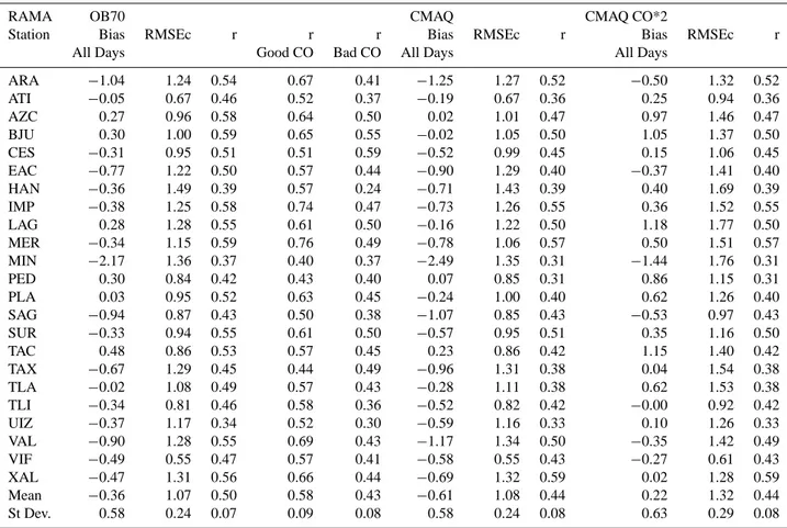
The bias, centred root mean square error (RMSEc, also called standard deviation of errors) and Pearson correlation coefficient of the model simulations are shown in Table 1 for each RAMA CO monitor for the 34 day period from 1 April to 4 May 2003. Fig. 6 shows the model perfor-mance using the statistical diagram introduced in de Foy et al. (2006b). The bias is plotted versus the RMSEc for each sta-tion. The standard deviations of the simulations are plotted versus those of the measurements to provide context to the magnitude of the errors. In order to compare the simulations, ellipses are drawn with centres at the mean of the perfor-mance metrics and radii corresponding to the standard devi-ations of the metrics.
Ideally, bias and RMSEc should be close to 0 and stan-dard deviations of the simulations should be equal to those of the model. Furthermore, RMSEc should be smaller than the standard deviations. From the table and figure, it can be seen that the negative bias of the CMAQ simulations is re-duced with OB70 and that errors are also slightly decreased. Doubling the emission inventory causes a positive bias and increases the RMSEc to greater than the standard deviations of the concentrations. Obs St Dev Model St Dev 0 0.5 1 1.5 2 −2.5 −2 −1.5 −1 −0.5 0 0.5 1 1.5 2 RMSEc ppm
Bias (Model − Obs) ppm
OB70 (Err) CMAQ (Err) CMAQ CO*2 (Err) OB70 (Std) CMAQ (Std) CMAQ CO*2 (Std)
Fig. 6. Statistics diagram for surface CO for 3 cases for all stations
with available data for the entire duration of the campaign. Each error point (Err) represents the bias versus the RMSEc (Standard deviation of errors) at a measurement station. Standard deviation points (Std) show the model standard deviation versus that of the measurements, which should be of similar magnitude.
Performance analysis of the meteorological simulations by episode type showed that the best simulations were obtained for the O3-South episodes and that simulations for the Cold Surge episodes were noticeably worse (de Foy et al., 2006a). As the same pattern is observable for CO simulations, the correlation coefficients for the OB70 simulations were sep-arated into days with good performance and days with poor performance, see Table 1. The 15 “Good CO” days were 13 to 16 April and 23 April to 4 May excluding 27 April. This includes both O3-South events and the second, and longest, O3-North event. The remaining 19 “Bad CO” days include the three Cold Surge episodes as well as the first O3-North episode which was the one that followed a period of heavy rains. The difference in correlation coefficients can be clearly seen. From this point on, the analysis will focus on the “Good CO” days.
Table 1 shows considerable variation in the performance metrics at different stations. For example, MER and IMP are located in the city centre near high emissions but are on a school and campus-like environment respectively, shield-ing them from emissions in the immediate vicinity. Poor performance at PED, which is in a leafy suburb with low emissions, suggests that the spatial distribution of the emis-sion inventory could be re-examined. Also poorly perform-ing is TAX, in this case quite possibly because it is located near a major bus transport hub. Finally stations such as MIN and SAG have noticeably weaker performance than near-by
Table 1. Comparison statistics of surface CO concentrations for 3 model cases versus all RAMA measurements available. Statistics calculated for the 34 day period (“All Days”) or for subsets (“Good CO” and “Bad CO”), see text.
RAMA OB70 CMAQ CMAQ CO*2
Station Bias RMSEc r r r Bias RMSEc r Bias RMSEc r
All Days Good CO Bad CO All Days All Days
ARA −1.04 1.24 0.54 0.67 0.41 −1.25 1.27 0.52 −0.50 1.32 0.52 ATI −0.05 0.67 0.46 0.52 0.37 −0.19 0.67 0.36 0.25 0.94 0.36 AZC 0.27 0.96 0.58 0.64 0.50 0.02 1.01 0.47 0.97 1.46 0.47 BJU 0.30 1.00 0.59 0.65 0.55 −0.02 1.05 0.50 1.05 1.37 0.50 CES −0.31 0.95 0.51 0.51 0.59 −0.52 0.99 0.45 0.15 1.06 0.45 EAC −0.77 1.22 0.50 0.57 0.44 −0.90 1.29 0.40 −0.37 1.41 0.40 HAN −0.36 1.49 0.39 0.57 0.24 −0.71 1.43 0.39 0.40 1.69 0.39 IMP −0.38 1.25 0.58 0.74 0.47 −0.73 1.26 0.55 0.36 1.52 0.55 LAG 0.28 1.28 0.55 0.61 0.50 −0.16 1.22 0.50 1.18 1.77 0.50 MER −0.34 1.15 0.59 0.76 0.49 −0.78 1.06 0.57 0.50 1.51 0.57 MIN −2.17 1.36 0.37 0.40 0.37 −2.49 1.35 0.31 −1.44 1.76 0.31 PED 0.30 0.84 0.42 0.43 0.40 0.07 0.85 0.31 0.86 1.15 0.31 PLA 0.03 0.95 0.52 0.63 0.45 −0.24 1.00 0.40 0.62 1.26 0.40 SAG −0.94 0.87 0.43 0.50 0.38 −1.07 0.85 0.43 −0.53 0.97 0.43 SUR −0.33 0.94 0.55 0.61 0.50 −0.57 0.95 0.51 0.35 1.16 0.50 TAC 0.48 0.86 0.53 0.57 0.45 0.23 0.86 0.42 1.15 1.40 0.42 TAX −0.67 1.29 0.45 0.44 0.49 −0.96 1.31 0.38 0.04 1.54 0.38 TLA −0.02 1.08 0.49 0.57 0.43 −0.28 1.11 0.38 0.62 1.53 0.38 TLI −0.34 0.81 0.46 0.58 0.36 −0.52 0.82 0.42 −0.00 0.92 0.42 UIZ −0.37 1.17 0.34 0.52 0.30 −0.59 1.16 0.33 0.10 1.26 0.33 VAL −0.90 1.28 0.55 0.69 0.43 −1.17 1.34 0.50 −0.35 1.42 0.49 VIF −0.49 0.55 0.47 0.57 0.41 −0.58 0.55 0.43 −0.27 0.61 0.43 XAL −0.47 1.31 0.56 0.66 0.44 −0.69 1.32 0.59 0.02 1.28 0.59 Mean −0.36 1.07 0.50 0.58 0.43 −0.61 1.08 0.44 0.22 1.32 0.44 St Dev. 0.58 0.24 0.07 0.09 0.08 0.58 0.24 0.08 0.63 0.29 0.08
stations MER and XAL, respectively. This can suggest im-pacts of neighbouring emissions or micro-meteorological ef-fects. MIN for example is located inside an elevated round-about (rotary/glorieta) with high traffic emissions very close to the monitor air-intake. Detailed comparison of the metrics with the station location and surroundings (see Sect. 3.4) in the future could point to possible weaknesses in both mod-elling and monitoring.
4.2.1 Column measurements
Comparisons of the statistical metrics for the 3 cases suggest that the OB70 scheme is better than the CMAQ scheme with or without adjustments in the emission inventory. These are entirely based on surface measurements however and do not account for the amound of CO in the atmosphere. A total column count of CO molecules can be used to evaluate the model simulations irrespective of their accuracy at the sur-face and hence to provide a constraint on the level of CO emissions.
Solar FTIR measurements of the CO columns are com-pared with simulated columns from the 3 model cases in
Fig-ures 7, 8 and 9. An offset of 0.52×10¹⁸molecules/cm2was applied to the model columns to account for the CO above the domain top, corresponding to free tropospheric concen-trations of 70 ppb above 440 hPa and 50 ppb above 120 hPa.
Agreement between model and observations is particu-larly good on 15 April. Unlike many urban areas where the columns increase throughout the day, CENICA experiences a steady reduction starting at noon. This is well captured by the model and is due to dilution caused by the gap flow (de Foy et al., 2006a). The small difference between the OB70 and CMAQ cases but the large difference with the CMAQ case with double CO emissions shows that the columns are sensi-tive to the emission levels and not the surface concentrations. The case with increased emissions clearly leads to excess CO in the atmosphere.
There was a sharp drop in emissions on 18 April which was Good Friday, a day when all schools and businesses are closed (de Foy et al., 2005). This can be seen in the mea-surements and is correctly captured by a 50% scaling fac-tor in the model. The diurnal trend of the columns suggests that the diurnal profile of the emissions needs to be adjusted however. Agreement on 21 April is not nearly as good. This
2 4 6 8 10x 10 18 CO Column (molec/cm2)
15−Apr−2003 CENICA 18−Apr−2003 CENICA SOF
OB70 CMAQ CMAQ, CO*2 00 03 06 09 12 15 18 21 00 2 4 6 8 10x 10 18 Time CDT CO Column (molec/cm2) 21−Apr−2003 CENICA 00 03 06 09 12 15 18 21 00 Time CDT 26−Apr−2003 CENICA
Fig. 7. Total column of CO measured by Solar Occultation Flux (SOF) versus model simulations for 3 simulation cases for different campaign days at CENICA.
2 4 6 8 10x 10 18 CO Column (molec/cm2)
16−Apr−2003 SATL SOF
OB70 CMAQ CMAQ CO*2 TPN OB70 17−Apr−2003 SATL 00 03 06 09 12 15 18 21 00 2 4 6 8 10x 10 18 Time CDT CO Column (molec/cm2)
27−Apr−2003 MER SOF
OB70 CMAQ CMAQ, CO*2 00 03 06 09 12 15 18 21 00 Time CDT 28−Apr−2003 MER
Fig. 8. Total column of CO measured by Solar Occultation Flux (SOF) versus model simulations for 3 simulation cases for different campaign days at Santa Ana (SATL) and La Merced (MER). TPN OB70 shows base case at Tlalpan, 20 km west of SATL, to highlight impact of gap flow.
2 4 6 8 10x 10 18 CO Column (molecules/cm2) 04/11 10:02 04/11 10:13 04/12 10:01 04/13 10:08 04/13 11:04 04/16 11:26 04/22 10:30 04/22 10:44 04/22 12:25 Date / Time CENICA 1 1.5 2 2.5 3x 10 18 CO Column (molecules/cm2) BC1 04/13 14:05 BC1 04/13 14:17 BC1 04/13 15:01 BC2 04/13 16:36 BC2 04/13 16:37 BC3 04/24 14:18 BC3 04/24 17:08 BC3 04/24 17:09 BC3 04/24 17:56 BC3 04/24 18:33 BC3 04/25 11:27 BC3 04/25 15:01 BC3 04/25 15:52 BC3 04/25 16:28 BC3 04/25 18:20 BC3 04/25 18:56 BC4 04/30 11:10 Site, Date / Time
BC
SOF OB870 CMAQ CMAQ, CO*2
Fig. 9. Total column of CO measured by Solar Occultation Flux (SOF) versus model simulations for individual measurements at CENICA
and at the boundary sites (see Fig. 1 for site locations).
1 2 3 4 5 6 7 x 10¹⁸ 1 2 3 4 5 6 7 8 9 10 11x 10 18
SOF CO Column (molec/cm2)
CAMx CO Column (molec/cm2)
OB70 CMAQ CMAQ CO*2
Fig. 10. Scatter plot of total column of CO measured by Solar Occultation Flux (SOF) versus model simulations for the 3 model cases. See Table 2 for coefficients of lines of best fit.
is attributable to the fact that this is a Cold Surge day with poorer model performance as described above.
At Santa Ana (SATL), on 16 April the columns show a slow decline after a 15:00 peak. On 17 April the afternoon
Table 2. Least squares fit (y=mx+c) for correlation of SOF CO
columns with 3 model simulations.
OB70 CMAQ CMAQ CO*2
m 0.78 0.71 1.37 95% bounds on m 0.58, 0.97 0.52, 0.90 0.99, 1.74
c(×1018) 1.24 1.43 0.62
r 0.36 0.33 0.32
decline is more gradual and follows a step increase at 12:00, when the urban plume reaches the southern basin rim. The trend is correctly captured on 16 April, but the simulated levels are too low. On 17 April, the levels are higher and the sharp increase occurs 2 hours earlier. Wind circulation at SATL are very sensitive to the strength and timing of the gap flow from the southeast (de Foy et al., 2006a). Columns 20 km to the west at TPN for the OB70 case show much higher levels on 16 April and somewhat higher levels on 17 April but a correct timing of the increase. This suggests that small changes in the gap flow can lead to large discrep-ancies in the model agreement.
At La Merced (MER), especially on 27 April, the simu-lated columns of CO are at the right level without adjusting the emission inventory. The columns rise and fall under the competing impact of traffic and wind transport (Garcia et al., 2006).
Boundary conditions in the model were verified by com-paring columns at boundary sites to the north of the MCMA
470 475 480 485 490 495 500 2130 2135 2140 2145 2150 2155 2160 2165 2170 2175 ARA ATI AZC BJU CES EAC HAN IMP LAG MER PED PLA SAG SUR TAC TAX TLA TLI UIZ VAL VIF XAL Bias=−1 Bias=−.4 Bias=.5 r=0 r=.5 r=1 UTME (km) UTMN (km)
Fig. 11. Bias (vertical lines) and correlation coefficient (horizontal
lines) CAMx OB70 vs. RAMA measurements for all stations except MIN, for “Good CO” days. Green for positive bias (model greater than observations), blue for negative bias smaller than 0.4 ppm and red for large negative bias. Correlation coefficient is plotted symet-rically around the origin, short horizontal bars indicate good agree-ment.
near Teotihuacan and Pachuca and outside the basin on the slopes of the Popocat´epetl. The agreement was good, with values ranging from 2.0×10¹⁸to 2.5×10¹⁸molecules/cm2.
Least squares fit of the simulations to the models are shown in Fig. 10 and Table 2 for the 3 cases along with 95% confidence bounds on the slope of the agreement. For the linear fit without constraining the y-intercept to 0, the un-certainty on the slopes are large and suggest that the base emission inventory could underestimate the actual CO levels. At 95% confidence level this would suggest that the method cannot distinguish between adjustment factors (a slope of 1 is within, or close to, the range for all 3 cases). If we constrain the y-intercept to 0 on the grounds that the boundary condi-tions are within 10% (0.25×10¹⁸molecules/cm2) of the true value (Fig. 9), then we obtain slopes in the range of 1.05 to 1.17 for OB70 and 1.42 to 1.64 for CMAQ with double CO. This provides stronger evidence that the current emis-sion inventory is at the right level and that no adjustments are currently warranted. 0 3 6 9 12 15 18 21 24 0 1 2 3 4 5 6 Time of Day (CDT) CO (ppm) CENICA FTIR CENICA UIZ (RAMA) CAMx OB70 0 3 6 9 12 15 18 21 24 0 1 2 3 4 5 6 Time of Day (CDT) CO (ppm) MER FTIR MER RAMA CAMx OB70
Fig. 12. Diurnal profiles of median concentrations of CO at MER
and CENICA comparing monitoring data, FTIR data and CAMx results for “Good CO” days.
4.2.2 Spatial analysis
Based on the analysis above, the case with unchanged emis-sions and OB70 vertical diffusion will be retained as the base case for further analysis. Figure 11 shows the bias and error for each station for the 15 days of the “Good CO” episodes. A clear pattern emerges, with positive bias (sim-ulations higher than measurements) for central and south-western stations and negative bias for northern and eastern stations. The correlation coefficient is highest (smaller bars) in the city centre and decreases in the periphery.
Median diurnal profiles of simulated and measured CO concentrations for CENICA and MER are shown in Fig. 12. At MER there is good agreement between the RAMA measurements, the FTIR and the model simulations. At CENICA, the early morning peak is clearly captured by all the measurements, but is not represented in the model. Dur-ing the rest of the day, the FTIR measurements are higher than the CENICA data but comparable to the RAMA data. This discrepancy should be investigated, especially if the measurements are used to validate the emission inventory.
0 3 6 9 12 15 18 21 24 0 1 2 3 4 5 6 7 8 Time of Day (CDT) CO (ppm) XAL (RAMA) CAMx OB70 0 3 6 9 12 15 18 21 24 0 1 2 3 4 5 6 7 8 Time of Day (CDT) CO (ppm) AZC (RAMA) CAMx OB70 0 3 6 9 12 15 18 21 24 0 1 2 3 4 5 6 7 8 Time of Day (CDT) CO (ppm) PED (RAMA) CAMx OB70 0 3 6 9 12 15 18 21 24 0 1 2 3 4 5 6 7 8 Time of Day (CDT) CO (ppm) VIF (RAMA) CAMx OB70
Fig. 13. Diurnal profiles of CO at selected RAMA stations for “Good CO” days. Bold line is the median, thin line the 25 and 75 percentile and dashed line the range. Measurements in yellow, model simulations in blue.
Further diurnal profiles for XAL, AZC, PED and VIF are shown in Fig. 13. At XAL, the pattern is well-captured but the predictions are too low. This is particularly acute in the morning with a delay in the rise of predicted concentrations. At PED, the opposite is true, with too high emissions in the early morning. VIF, to the north of the city, has much lower concentrations. Nonetheless, they are under-predicted by the model. At AZC, the morning peak starts too soon and rises too high, whereas at neighbouring VAL (not shown), the tim-ing is correct but concentrations drop off much faster than the measurements. This illustrates the pitfalls of comparing grid-ded model results with point measurements and the need to consider carefully station location.
4.3 Discussion
The Concentration Field Analysis for CO shows that the method is able to correctly identify known sources based on surface data from the monitoring network. The method was shown to be robust with respect to station location and the prevailing wind directions. The analysis can be applied to individual stations first with model concentrations and then with actual measurements in order to identify the upwind re-gions that affect a monitor and wether the measurements are dominated by local or more regional transport.
Column measurements of CO were shown to provide a necessary constraint in evaluating potential adjustment fac-tors to the emission inventory. Uncertainty in the model sim-ulations based on statistical metrics and data comparisons can be estimated to be between 35% and 50%. The high errors in the model have been attributed to complex mete-orology in the basin (de Foy et al., 2006a). While this pre-cludes a definite conclusion on the adjustment factors for CO emissions, it nonetheless suggests that current levels are con-sistent with concentrations.
Spatial patterns of Eulerian model performance can be used to evaluate the spatial distribution of the inventory. Positive bias in the southwest and negative bias to the east and north are consistent with current patterns of urbanisa-tion. This suggests possible adjustments in terms of city sec-tors, although it is too crude to resolve features on the scale of individual grid cells. The effect can be clearly seen at CENICA. In the simulations, the station is on the edge of the city edge and does not see the strong morning rush hour peak in measured CO.
Comparisons of diurnal profiles at individual stations can be used to evaluate the temporal distribution of the emis-sions and to suggest modifications by time of day. Vary-ing emissions durVary-ing vacations and holidays are a source of uncertainty and model under-performance that has not been quantified in the present study. Scaling factors for high and low emission days were deduced from morning CO observa-tions. Traffic data will be needed to refine these as the biggest change in emissions by day of week and type of day may be
VIF SATL VIF 0.2 0.3 0.4 0.5 0.6 0.7 0.8 0.9 1.0 No SATL
Fig. 14. Concentration Field analysis of SO2based on measured concentrations and simulated back-trajectories at VIF (left) and SATL (right) showing possible northwest source region.
the temporal and spatial distribution rather than the overall emission level.
5 Sulfur dioxide
5.1 Concentration field analysis
Concentration field analysis was performed for SO2 in the
same way as for CO, see Sect. 4. Results for VIF and SATL, the stations most to the north and south respectively, are shown in Fig. 14. Both of these point to a focused source to the northwest of the city. The signal at VIF is particularly clear, with only small contributions from areas southwest of the station. Because SATL is further away and on the south-ern edge of the basin rim, the picture is more diffuse. The trace from the northwest is still clearly visible however, with suggested transport southwards along the western edge of the basin.
5.2 Eulerian modelling
CAMx simulations of SO2were carried out with the OB70
vertical diffusion scheme. In addition to the point and area sources from the emissions inventory, point sources for the Tula industrial complex and for the Popocat´epetl volcano were added as described in Sect. 3. Generic stack parameters were used which do not affect the long range transport of the plume. Emissions were set to 5 kg/s for Tula and 10 kg/s for Popocat´epetl based on the mini-DOAS estimates. The emissions were held constant in time. These emissions cor-respond to 158×103tonne/year and 316×103tonne/year re-spectively. All boundary and initial conditions for SO2were
set to 1 ppb based on GOME satellite retrievals available at the Belgian Institute for Space Aeronomy (IASB-BIRA).
Figure 15 shows time series of SO2 at VIF to the north
of the city and CENICA to the southeast for measurements
0 20 40 60 80 100 120 140 160 180 200 220 240 VIF SO2 (ppb) Obs CAMx MCMA Frac Tula Frac Popo Frac 01 03 05 07 09 11 13 15 17 19 21 23 25 27 29 01 03 05 0 20 40 60 80 100 Day CENICA SO2 (ppb)
Fig. 15. SO2time series at VIF and CENICA showing measured (black) versus modelled (red) concentrations for the entire cam-paign. Coloured shading indicates the fraction of simulated SO2 that is due to different sources (MCMA, Tula and Popocat´epetl).
and simulations that include the Tula and Popo point sources. The shading in the background indicates the fraction of the simulated SO2 due to the Tula industrial complex and the
volcano obtained by running separate tracer simulations. This shows that the model would not simulate the sharp peaks if emissions from Tula were not included. At VIF,
0 3 6 9 12 15 18 21 24 0 5 10 15 20 25 Time of Day (CDT) SO2 (ppb) MER FTIR CAMx OB70 0 3 6 9 12 15 18 21 24 0 1 2 3 4 5 6 7 8 9 10 Time of Day (CDT) SO2 (ppb) DOAS−1 DOAS−2 CENICA CAMx OB70
Fig. 16. Diurnal profiles of SO2at MER and CENICA compar-ing monitorcompar-ing data, DOAS data and model results for “Good CO” days. Bold line is the median, thin line the 25 and 75 percentile.
there are 7 of these above 50 ppb during the campaign. By the time they reach CENICA, their impact is reduced except for events occurring during Cold Surge episodes when ver-tical mixing is low and transport is directly from the north (de Foy et al., 2006a). There are episodes where the model indicates volcanic impacts on the urban area, although these correspond to low SO2concentrations. It is therefore difficult
to differentiate them from the urban emissions.
Figure 16 shows the comparison in measured and simu-lated diurnal SO2concentrations at CENICA and MER. At
CENICA, the morning peak is much more pronounced in the measurements from the monitoring station data than in the DOAS measurements. The simulated concentrations are in reasonable agreement with the DOAS measurements al-though the morning peak is under-predicted. At MER, levels of SO2measured by DOAS are similar to those at CENICA.
The simulation levels however are substantially higher sug-gesting that the spatial distribution of the emission inventory should be re-evaluated for SO2in a similar fashion as for CO.
10−Apr−2003 04:00:00 10−Apr−2003 07:00:00 10−Apr−2003 10:00:00 CAMX−OB70 RAMA (4 − 183 ppb) (22 − 193 ppb) (11 − 249 ppb) (9 − 197 ppb) (17 − 102 ppb) 0 25 50 75 100 125 150 ppb (17 − 144 ppb)
Fig. 17. Surface concentration of SO2 from model (left) and RAMA observations (right) at 04:00, 07:00 and 10:00 CDT dur-ing the SO2plume episode of 10 April 2003. Numbers in brackets show the domain-wide minimum and maximum concentrations of the measurements for the RAMA plots, and of the model area cor-responding to the measurement locations for the CAMx plots.
5.3 SO2plume event
10 April experienced a large SO2plume that swept past the
whole city with peak concentrations above 200 ppb in the northern part of the MCMA. Contour plots for 04:00, 07:00 and 10:00 are shown in Fig. 17 for RAMA measurements and model simulations. Figure 18 shows the time series of SO2 concentrations at points on the northern boundary of
the MCMA as well as at different stations along a north– south transect. The initial rise is at TLI, to the west of the Sierra de Guadalupe at around 22:00 of the previous day. Two hours after this there is a substantially larger rise that now extends to VIF to the north, which experiences the bulk of the plume after 03:00. The plume then shifts further east to XAL before returning west to VIF at around sunrise fol-lowed by dispersion due to vertical mixing. The impact can be seen at MER building up through the night along with fluctuations due to plume meandering. At CENICA the lev-els are lower and smoother due to the longer transport dis-tance. This is even more so at PED which starts to see the
18:000 21:00 00:00 03:00 06:00 09:00 12:00 15:00 18:00 50 100 150 200 250 300 350
Time of Day, CDT (10 April 2003)
SO2 (ppb) TLI VIF XAL MER CENICA PED
Fig. 18. Time series of measured SO2concentrations at 1-min resolution for 10 April plume event at selected RAMA stations and at CENICA.
plume around 03:00 and reaches a maximum between 09:00 and 12:00. Long-path DOAS measurements at CENICA are in remarkable agreement with the point measurement. In addition to adding confidence to the accuracy of the mea-surements, this highlights the fact that the plume is a large scale phenomenon. Both the measurements and the simula-tions suggest that the SO2 plume originated to the north of
the MCMA.
As can also be seen in the time series in Fig. 15, the tim-ing and extent of the plume is correctly captured although the maximum levels are under-predicted. The measurement con-tours show the plume going around both sides of the Sierra de Guadalupe and then moving towards the east. In the model, there is some splitting of the plume around the mountains, but the main effect of the Sierra de Guadalupe is to cause strong vertical mixing leading to a much more diffuse plume. This explains the lower levels observed over the city and the reduced extent of an SO2-rich air mass separated from the
plume moving northeastward at 10:00. This case suggests that the effect of terrain on transport in the stable boundary layer may not be correctly represented numerically.
5.4 Discussion
Both Concentration Field analysis with backward trajecto-ries and forward Eulerian modelling using emission esti-mates from zenith sky UV spectroscopy suggest that there is a SO2 plume from the Tula industrial complex that can
impact the MCMA. These plumes are typically in the early morning or late evening under stable conditions when wind flows are from the north. While the effect is strongest on the stations in the north of the city, there are occasions where the entire MCMA is affected. Without considering the possible variation in SO2emissions, the current simulations captured
many of the plumes in the MCMA. The impact on the city is limited to episodes with stable northerly flow. The major-ity of the time the plume would be expected to follow the prevailing westerlies.
In modelling terms, the SO2 plume presents a valuable
case study for the effect of complex terrain on plume
trans-Table 3. SO2annual emissions estimates from fuel consumption in the MCMA and at the Tula power plant compared with the official inventory for the MCMA and the Mini-DOAS estimate for the Tula industrial complex.
MCMA Tula Power Plant Fuel Consumption (tonne/yr) 5.7×10⁶ 1.49×10⁶ Emission Factor (kg SO2/tonne fuel) 0.71 86.26
Annual SO2Emissions (tonne/yr) 4050 128 000
CAM 2000 Inventory 4929
Mini-DOAS Estimate 145 000
port under stable conditions. Further study into the vertical dispersion as well as the vertical resolution of the dispersion model could be validated from the surface measurements of SO2.
Possible impacts from volcanic emissions were identified, although the levels are too low to differentiate from ambient measurements. During the dry season, winds aloft are pre-dominantly westerly and transport the emissions away from the city towards Puebla and beyond. During the field cam-paign the possible effects were found mainly during the Cold Surge episodes which are characterised by southward winds and stable conditions. It should be noted however that vol-canic emissions from the Popocat´epetl have been reported to be 10 to 100 times larger than the value used in this study, suggesting that much larger impacts are possible during spe-cific episodes.
Annual SO2 emission estimates for MCMA mobile
sources and for the Tula power plant are shown in Table 3. A fleet-average emission factor is derived from long-path DOAS measurements of SO2 and CO2 (Volkamer et al.,
2005a). Multiplying this by known fuel consumption in the city during April 2003 and scaling to an annual value leads to an emission estimate 20% lower than the official inventory, which is deemed to be within the accuracy of the simulations and the measurements. An estimate of the power plant emis-sions was obtained by combining the annual fuel consump-tion and average sulfur content of the fuel. The emissions of the refinery are not included in this estimate. Overall, this is in agreement with the estimate from UV-Spectroscopy plume measurement given the limits of accuracy.
Summing SO2impacts at MER and CENICA from model
simulations for the Tula and Popocat´epetl point sources sug-gests that in the simulations 75% of SO2concentrations are
due to local sources during April 2003, with possibly 20% from the power plant and 5% from the volcano.
6 Conclusions
Analysis of CO showed that vertical dispersion schemes in air quality models can have a large impact on simulated