Coastal zone production of IO precursors: a 2-dimensional study

(1)

HAL Id: hal-00295173

https://hal.archives-ouvertes.fr/hal-00295173

Submitted on 23 Nov 2001

HAL is a multi-disciplinary open access

archive for the deposit and dissemination of

sci-entific research documents, whether they are

pub-lished or not. The documents may come from

teaching and research institutions in France or

abroad, or from public or private research centers.

L’archive ouverte pluridisciplinaire HAL, est

destinée au dépôt et à la diffusion de documents

scientifiques de niveau recherche, publiés ou non,

émanant des établissements d’enseignement et de

recherche français ou étrangers, des laboratoires

publics ou privés.

Coastal zone production of IO precursors: a

2-dimensional study

L. J. Carpenter, K. Hebestreit, U. Platt, P. S. Liss

To cite this version:

L. J. Carpenter, K. Hebestreit, U. Platt, P. S. Liss. Coastal zone production of IO precursors: a

2-dimensional study. Atmospheric Chemistry and Physics, European Geosciences Union, 2001, 1 (1),

pp.9-17. �hal-00295173�

(2)

Atmos. Chem. Phys., 1, 9–18, 2001

www.atmos-chem-phys.org/acp/1/9/

Atmospheric

Chemistry

and Physics

Coastal zone production of IO precursors: a 2-dimensional study

L. J. Carpenter1, K. Hebestreit2, U. Platt2, and P. S. Liss3

1_{Department of Chemistry, University of York, York, YO10 5DD, UK}

2_{Institut f¨ur Umweltphysik, University of Heidelberg, INF 229, D-69120 Heidelberg, Germany} 3_{School of Environmental Sciences, University of East Anglia, Norwich, NR4 7TJ, UK} Received 13 August 2001 – Published in Atmos. Chem. Phys. Discuss. 3 September 2001 Revised 8 November 2001 – Accepted 9 November 2001 – Published 23 November 2001

Abstract. At Mace Head, Eire, in the coastal East Atlantic, diiodomethane has been identified as an important precursor of iodine oxide radicals. Peak concentrations of both CH2I2

and IO at low water indicate that the intertidal region is a strong source of organo-iodines. Atmospheric measurements of CH2I2made in marine air are compared with the

concen-trations predicted by a 2-dimensional model incorporating horizontal and vertical dispersion of surface emissions. The model shows that micrometeorological variability, proxim-ity of the site to emissions, and photolysis all play important roles in determining the CH2I2concentrations at Mace Head.

In addition to a tidal-height dependent intertidal flux, which was estimated from seaweed production data, a contribution from offshore (non-local) sources was required in order to reproduce the strong signature of photolysis in the CH2I2

observations. A combination of an offshore flux and an in-tertidal flux (of up to 1.4 × 109_{molecules cm}−2_s−1_{at low}

water) results in good agreement between the measured and modelled CH2I2 concentrations. Although this study does

not necessarily infer emission of CH2I2from the open ocean,

it suggests that air-sea exchange of CH2I2in coastal waters

does occur.

1 Introduction

During the last decade it was established that catalytic cycles involving halogen oxide radicals (BrO with smaller contri-butions from IO and ClO) were responsible for rapid ozone depletion events in the Arctic boundary layer during spring (Barrie et al., 1988; Bottenheim et al., 1990; Barrie and Platt, 1997). More recently, the IO radical has been identified in Antarctica (Friess et al., 2001) and in the mid-latitudes (Alicke et al., 1999; Allan et al., 2000) in conjunction with organoiodine precursors (Carpenter et al., 1999), confirming Correspondence to: L. J. Carpenter (ljc4@york.ac.uk)

the potential for the more widespread occurrence of bound-ary layer ozone depletion. Formation of IO is driven by ocean-atmosphere exchange of organo-iodines that are pho-tolysed quickly within the marine boundary layer. Previous studies at Mace Head found that a range of photolabile io-dine containing organics including CH3I, C2H5I, CH2ICl, CH2IBr and CH2I2were present in sufficiently high

concen-trations to sustain IO levels of a few parts per trillion (ppt), via the following reactions:

RI−→ R + Ihv (1)

I + O3→ IO + O2 (2)

Of the organoiodines measured, CH2I2was found to be the

most important iodine precursor (Carpenter et al., 1999). The photodissociation lifetime of diiodomethane is only a few minutes at midday (M¨ossinger et al., 1998).

The impact of IO on ozone concentrations depends on the detailed gas phase and heterogeneous chemistry following reaction (2). Computational modelling investigations indi-cate that the rate of ozone destruction associated with iodine photochemistry in the marine boundary layer could equal that from HOx photochemistry (Vogt et al., 1999; Stutz et al.,

1999; McFiggans et al., 2000). Perhaps of even greater un-certainty are the emissions and distributions of iodine precur-sors. Shipboard experiments have identified CH2ICl (Klick

and Abrahamsson, 1992; Schall et al., 1997) and CH2I2

(Schall et al., 1997) in the open ocean, although it is not yet established whether these originate from microalgae (phy-toplankton) or other (e.g. photochemical) sources. That coastal macroalgae are prolific emitters of a wide range of or-ganic halogens is without doubt (e.g. Gschwend et al., 1985; Nightingale et al., 1995; Peders´en et al., 1996; Carpenter et al., 2000 and references therein), although the global budgets of seaweed emissions are very uncertain.

During the ACSOE (Atmospheric Chemistry Studies in the Oceanic Environment) experiment at Mace Head in 1997,

c

(3)

10 L. J. Carpenter et al.: Coastal zone production of IO precursors

L. J. Carpenter et al., Coastal zone production of IO precursors 1

0,0 2,0 4,0 6,0 0,0 1,0 2,0 3,0

9 Sep 10 Sep 11 Sep 12 Sep 13 Sep 14 Sep 15 Sep

9 Sep 10 Sep 11 Sep 12 Sep 13 Sep 14 Sep 15 Sep 0 20 40 60 80 photopic [klx] tidal height [m] Date 1998, UT IO [ppt]

Figure 1. IO, tidal height and solar radiation (as photopic flux) during 9-15 September, 1998.

The dotted line on the IO graph represents the average detection limit. The grey areas mark the low tide periods during the day.

Fig. 1. IO, tidal height and solar radiation (as photopic flux) during

9–15 September 1998. The dotted line on the IO graph represents the average detection limit. The grey areas mark the low tide periods during the day.

macroalgal emissions were observed to have a direct impact on the local atmosphere, as reflected by the peak air con-centrations of polyhalogenated halocarbons occurring at low water (Carpenter et al., 1999). These observations may be attributed to direct emission into the surrounding air from exposed macroalgae at low tide and/or increased emissions due to oxidative stress of algae upon exposure (Carpenter et al., 2000). At high tide, emissions from submerged beds are diluted in seawater and may undergo photolysis before ex-change at the air-sea interface.

Measurements of organo-iodines and IO radicals at Mace Head were repeated during the 1998 EU project PARFORCE (New Particle Formation and Fate in the Coastal Environ-ment). In this study we attempt to evaluate the relative im-portance of coastal and offshore emissions of CH2I2,

pro-viding further information on sources of the IO radical. A 2-dimensional model is used to predict the horizontal and ver-tical distributions of CH2I2 resulting from coastal and

off-shore (non-local) emissions.

2 Experimental

Mace Head is located on the remote western coast of County Galway, Eire (53◦190N, 9◦540W). The site is well known for background air measurements and receives relatively clean marine air from the prevailing westerly sector associated with the easterly tracking cyclonic systems of the North

At-L. J. Carpenter et al., Coastal zone production of IO precursors 2

0 1 2 3 4 5 0,0 0,5 1,0 1,5 2,0 2,5 a a _a a a _a a _a a _a a d d d d d d d d d d d n n n n n n n n n _{n n} tidal height [m] [IO] = 2.6 x e(-[TH]/1.7) (r² = 0.96) (d) = 1.2 x e(-[TH]/2.2) (r² = 0.94) (a) = 0.08 (r² = 0.89) (n) IO [ppt] n = night d = day a = all data

Figure 2. Correlation of IO and tidal height (TH) during PARFORCE (whole data set). The data

points are binned averages of 0.5m segments of TH. The vertical error bars represents the relative frequency of the data, the horizontal error bars the length of the respective interval. The daytime data and all data are fitted with an exponentially decreasing trend, the night-time data has a linear fit.

Fig. 2. Correlation of IO and tidal height (TH) during PARFORCE

(whole data set). The data points are binned averages of 0.5 m segments of TH. The vertical error bars represents the relative fquency of the data, the horizontal error bars the length of the re-spective interval. The day-time data and all data fitted with an ex-ponentially decreasing trend, the night-time data has a linear fit.

lantic. The rocky upper littoral zone and cold waters provide favourable conditions for seaweeds.

2.1 Halocarbons

During the period 5–24 September 1998, halocarbons in air were monitored in-situ every 40 minutes with a Hewlett Packard 6890/5973 gas chromatograph/mass spectrometer (GC/MS) system. The GC/MS was operated in a laboratory situated ca. 100 m from the high tide mark, with a sampling inlet located with an open fetch to the ocean at a height of approx. 12 m above mean sea level (MSL). The system is de-veloped for automated air sampling and is described fully in Carpenter et al. (1999). Analysis was also performed on dis-crete samples of surface seawater and the water surrounding incubated seaweeds. For a full description of analytical pro-cedures for air and seawater analyses during PARFORCE see Carpenter et al. (2000).

2.2 IO measurements by DOAS

Over a 1-month period from 8 September until 8 October 1998 LP DOAS (Long-Path Differential Optical Absorption Spectroscopy; Platt, 1994) measurements of the halogen

(4)

ox-L. J. Carpenter et al.: Coastal zone production of IO precursors

L. J. Carpenter et al., Coastal zone production of IO precursors

11

3 Figure 3. CH

2

I

2

, tidal height and calculated J-CH

2

I

2

during clean maritime conditions.

0.0 0.1 0.2 0.3 0.4 0.5 9/18/98 0:00 9/19/98 0:00 9/20/98 0:00 9/21/98 0:00 CH 2 I2 [ppt], TH *0.1 [m] 0.0E+00 2.0E-03 4.0E-03 6.0E-03 J-CH 2 I2 [s -1 ] TH CH2I2 JCH2I2

Fig. 3. CH2I2, tidal height and calculated J-CH2I2during clean marine conditions.

ides IO, OIO and BrO and of other atmospheric trace gases including NO2, O3, HCHO, HONO and NO3 were carried

out whenever the visibility allowed reasonable signal to noise ratios.

Briefly, the principle of DOAS is the identification and quantification of atmospheric trace gases by their specific narrow (< 5 nm) band optical absorption structure in the open atmosphere, separating trace gas absorption from broad band molecule and aerosol extinction processes, thus allow-ing very sensitive detection of many molecular species (see e.g. Platt and Perner, 1983). The identification of the gases is unambiguous since their specific absorption structure is, similar to a fingerprint, unique. Calibration of the instrument is not necessary as long as the absorption cross section is known.

A DOAS instrument based on the principle of Platt and Perner (Platt and Perner, 1983) was used at Mace Head. It incorporates a combination of two coaxially arranged New-tonian telescopes, one collimating the light of a Xe-short-arc lamp through the atmosphere, the second recollecting the beam reflected by an array of quartz prism retroreflectors. The telescopes were set up in a laboratory about 20 meters from the shore, while the retroreflector array was placed on the northern shore of the bay. The light beam was running at an average height of 10 meters above the ocean with a light path length of 2 × 7.27 km. A 0.5 m Czerny-Turner spectrograph (f = 6.9, 600 gr/mm grating, thermostated to

30 ± 0.3◦C), in combination with a 1024 pixel photodiode

array detector (thermostated to −15 ± 0.3◦C), was coupled to the telescope by a quartz fibre, which also performed the task of a mode mixer (Stutz and Platt, 1997). Iodine oxide was measured in the wavelength range from 414 to 437 nm with a spectral resolution of about 0.5 nm (a dispersion of

0.078 nm/pixel). Three further wavelength regions were cho-sen to detect BrO (335 ± 40 nm) (H¨onninger, 1999), OIO (550 ± 40 nm) (Hebestreit, 2001), NO3(645 × 40 nm) and

the other species absorbing in the respective wavelength re-gions (O3, SO2, NO2, HCHO, HONO). Besides NO3, all

spectra were recorded using the multi channel scanning tech-nique (Brauers et al., 1995). The concentrations of IO were derived using a least squares fit mixer (Stutz and Platt, 1997) of the reference spectra of H2O, NO2and IO, together with

a sixth order polynomial to the atmospheric absorption spec-trum. The IO reference spectrum was measured in our labo-ratory, since no absorption cross section of sufficient resolu-tion was available. NO2 was measured in a reference cell

in the field. Absolute values for both spectra were deter-mined by comparison with literature cross sections (Cox et al., 1999; Harder et al., 1997; H¨onninger, 1999). The H2O

reference was calculated by a convolution of the instrument function with the absorption cross section of the HITRAN database (HITRAN, 1987).

2.3 Model description

A 3-day period (18–20 September 1998, Julian days 261–263) of clean marine south-westerly air with sta-ble temperatures (17.2 ± 1.9◦C) and wind speed (5.5 ±

1.0 m s−1) was selected as a case study for evaluation

of marine emissions. Data were evaluated using a model written in the FACSIMILE language. The pho-tolysis rate of diiodomethane (J-CH2I2) was computed

at 40 minute intervals using a 2-stream radiative trans-fer model (Hough, 1988), with absorption cross-sections from M¨ossinger et al. (1998) and TOMS O3 column data

(http://toms.gsfc.nasa.gov/ozone/ozone01.html). Photolysis rates were corrected for cloud cover using the ratio of

(5)

12 L. J. Carpenter et al.: Coastal zone production of IO precursors L. J. Carpenter et al., Coastal zone production of IO precursors 4

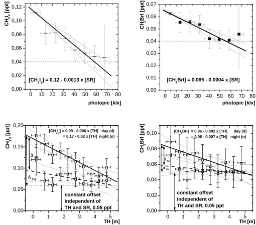
0 10 20 30 40 50 60 70 80 0,00 0,02 0,04 0,06 0,08 0,10 0,12 0 10 20 30 40 50 60 70 80 0,00 0,01 0,02 0,03 0,04 0,05 0,06 0,07 CH 2 I2 [ppt] [CH 2I2] = 0.12 - 0.0013 x [SR] photopic [klx] [CH₂BrI] = 0.065 - 0.0004 x [SR] photopic [klx] CH 2 BrI [ppt]

Figure 4. Correlations of CH2I2 and CH2IBr with solar radiation (SR) and tidal height (TH) for

the whole measurement period. The data points are binned averages of 0.5m segments of TH. The vertical error bars represents the relative frequency of the data, the horizontal error bars the length of the respective interval. The correlation with TH is divided into night-time (n) and day-time (d) values of CH2I2 and CH2IBr, respectively.

0 1 2 3 4 5 0,00 0,05 0,10 0,15 0,20 0 1 2 3 4 5 0,00 0,02 0,04 0,06 0,08 0,10 0,20 n n n n _n n n n _n n d d d d d d d _d d d n n n n n n _n n n n d d d d d d d d d d TH [m] ∆∆ SR ∆∆ TH constant offset independent of TH and SR, 0.06 ppt [CH2I2] = 0.09 - 0.006 x [TH] day (d) = 0.17 - 0.02 x [TH] night (n) CH 2 I2 [ppt] ∆∆ SR ∆∆ TH constant offset independent of TH and SR, 0.05 ppt TH [m] [CH 2BrI] = 0.06 - 0.002 x [TH] day (d) = 0.08 - 0.007 x [TH] night (n) CH 2 BrI [ppt]

Fig. 4. Correlations of CH2I2and CH2IBr with solar radiation (SR) and tidal height (TH) for the whole measurement period. The data points

are binned averages of 0.5 m segments of TH. The vertical error bars represents the relative frequency of the data, the horizontal error bars the length of the respective interval. The correlation with TH is divided into night-time (n) and day-time (d) values of CH2I2and CH2IBr,

respectively.

sured/modelled UVA data. The 2-dimensional model incor-porated a 5.2 km long by 50 m high slice through the atmo-sphere divided into cells of 100 m length and 2 m height. The first 5 km of the horizontal axis represented the “offshore” re-gion, the next 100 m represented the intertidal rere-gion, and the Mace Head site was notionally located in the final 100 m cell, at 12 m height (the sampling height of CH2I2). CH2I2was

emitted into the bottom cell and transported across consec-utive cell faces using the finite volume method to discretise the spatial partial derivatives, given by:

∂C ∂t = Q + D ∂2_C ∂x2 − u ∂C ∂x (3)

where C is the concentration of CH2I2, Q is the net rate

of production and destruction, D is the diffusion coefficient (set to zero for horizontal transport), the third term represent-ing advection, with u the horizontal wind speed. Horizontal wind speed was parameterised with 40-minute averages of the measured mean values at 3 m height (de Leeuw et al., 2001). Measurements made at 18 m were typically ∼ 25% higher (de Leeuw et al., 2001) as expected from the loga-rithmic dependence of wind speed with height and a rough-ness length, z0, of ∼ 10−4m (Kunz et al., 2000). Locally,

the extent of the sloping terrain upwind of the site will vary with tidal height, adding to some variability in the roughness length.

The rate of transport across the vertical boundary faces of each cell was described by replacing ∂x with ∂z and the eddy diffusivity coefficient, Kz, in place of D. The diffusivity

coefficient was assumed to vary with height in the surface layer according to (cf. Stull, 1988):

Kz=

κu∗z

φ(z/L) (4)

where κ is the von Karman constant (κ = 0.4), z is height,

u∗ is the friction velocity and φ(z/L) is a stability

correc-tion equal to unity during neutrally stratified boundary layer conditions, which prevailed at Mace Head (de Leeuw et al., 2001). During PARFORCE, de Leeuw et al. (2001) found that the friction velocity in marine sector air was approxi-mately equal to 9% of the wind speed at 3 m, a relationship which was used to define u∗ in the model. Formation of an internal boundary layer (IBL) would lead to abrupt changes in the diffusivity gradient at heights determined by the dis-tance from the shoreline. It is difficult to assess the impact of

(6)

L. J. Carpenter et al.: Coastal zone production of IO precursors 13 L. J. Carpenter et al., Coastal zone production of IO precursors 5

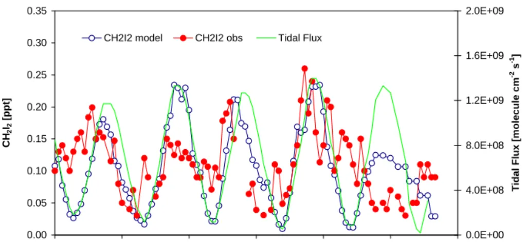
Figure 5. Comparison of measured and modelled CH2I2 levels assuming only tidal emissions,

shown with the tidal flux used in the model.

0.00 0.05 0.10 0.15 0.20 0.25 0.30 0.35 9/18/98 0:00 9/18/98 12:00 9/19/98 0:00 9/19/98 12:00 9/20/98 0:00 9/20/98 12:00 9/21/98 0:00 CH 2 I2 [ppt] 0.0E+00 4.0E+08 8.0E+08 1.2E+09 1.6E+09 2.0E+09

Tidal Flux [molecule cm

-2 s -1]

CH2I2 model CH2I2 obs Tidal Flux

Fig. 5. Comparison of measured and modelled CH2I2levels assuming only tidal emissions, shown with the tidal flux used in the model.

Figure 6. Comparison of measured and modelled CH2I2 levels assuming only offshore emissions

(constant wind speed and K).

0.00 0.05 0.10 0.15 0.20 0.25 0.30 9/18/98 0:00 9/18/98 12:00 9/19/98 0:00 9/19/98 12:00 9/20/98 0:00 9/20/98 12:00 9/21/98 0:00 [ppt]

CH2I2 obs CH2I2 model

Fig. 6. Comparison of measured and modelled CH2I2levels assuming only offshore emissions (constant wind speed and K).

IBL formation on the conclusions of this study, but we note the additional uncertainty.

3 Results and discussion

3.1 Relationships of iodine species with tidal height and solar radiation

Analysis of PARFORCE data showed that tidal height (TH) and solar radiation (SR) were correlated with CH2I2, IO, and

to a lesser extent, CH2IBr air concentrations. Figure 1 shows

IO, tidal height and solar radiation at 555 nm (photopic flux in kW/m2_{= klx) for the period 9–15 September. The figure}

shows that the maximum IO concentrations occurred during the day at low tide. The daily IO maximum shifted simul-taneously with the minimum in TH (about one hour from day to day), indicating that both solar flux and tidal height controlled the time of the IO peak. There is an IO peak af-ter sunset on the evening of the 14 September, however the IO signal during this period was below the detection limit,

which increased substantially at that time due to fog. Fig-ure 2 shows correlations of IO versus TH for daytime val-ues only (d), all data (a), and night-time valval-ues (n) of the 4 week measurement period. Under daylight conditions, high IO values were clearly associated with low tidal height, while at night no correlation between IO and TH was found. The correlation was described well by an exponential decrease with rising tide (r2_{= 0.96).}

Figure 3 shows tidal height, CH2I2 concentrations and

calculated J-CH2I2during the clean marine south-westerly

air period 18–20 September 1998. Scatter plots for CH2I2

and CH2IBr concentrations with TH and SR for the whole

campaign period are shown in Fig. 4. Strong evidence for these organic iodines as important photolytic precursors of IO is evident from their decreasing concentrations with solar flux and, during night-time, maxima at low tide. There is lit-tle correlation between TH and organo-iodine levels during the day, because of the strong influence of photolysis. Note that although peak concentrations of organo-iodines were observed at low water, both CH2I2 and CH2IBr exhibited

(7)

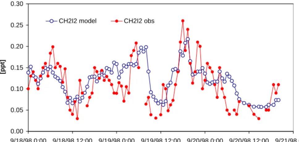
Figure 7. Comparison of measured and modelled CH2I2 levels assuming only offshore emissions (40 minute averaged wind speed and K).

0.00 0.05 0.10 0.15 0.20 0.25 0.30 9/18/98 0:00 9/18/98 12:00 9/19/98 0:00 9/19/98 12:00 9/20/98 0:00 9/20/98 12:00 9/21/98 0:00 [ppt]

CH2I2 model CH2I2 obs

Fig. 7. Comparison of measured and modelled CH2I2levels assuming only offshore emissions (40 minute averaged wind speed and K).

Figure 8. Comparison of measured and modelled CH2I2 levels assuming both offshore and

intertidal emissions (40 minute averaged wind speed and K).

0.00 0.05 0.10 0.15 0.20 0.25 0.30 9/18/98 0:00 9/18/98 12:00 9/19/98 0:00 9/19/98 12:00 9/20/98 0:00 9/20/98 12:00 9/21/98 0:00 CH 2 I2 obs [ppt] 0.00 0.05 0.10 0.15 0.20 0.25 0.30 0.35 0.40 CH 2 I2 model [ppt]

CH2I2 obs CH2I2 model

Fig. 8. Comparison of measured and modelled CH2I2 levels assuming both offshore and intertidal emissions (40 minute averaged wind

speed and K).

non-zero concentrations above their detection limits of 0.03 pptv even at high tide, presumably due to local sources, as discussed later. The dependence of CH2I2 on tidal height

and solar radiation was found to be [CH2I2]night = 0.17 − 0.02[TH] and [CH2I2]all= 0.12 − 0.0013[SR].

Given that the organoiodine precursors exhibited linear de-pendencies with TH at night, the cause of the exponential relationship of IO with TH (Fig. 2) does not appear to be ex-plained by source variations and is possibly attributable to the photochemistry of IO. It should also be noted that the IO measurements represent averages over ∼ 7 km, whereas the organoiodines were measured by point sampling.

3.2 2-dimensional model simulations

The initial model simulations incorporated only tidal emis-sions. The night-time CH2I2vs TH negative trend, shown

in Fig. 4, was presumed to be indicative of coastal produc-tion processes. Therefore the tidal dependence of the coastal flux was assumed to have the same qualitative form. A

quan-titative fix was available from independent data on seaweed emissions, described below.

In addition to atmospheric measurements made during PARFORCE, the release rates of organic bromines and iodines from seaweeds were determined from incubations in seawater of ten species of brown, red and green macroal-gae collected in the intertidal or subtidal zones of the rocky shore (Carpenter et al., 2000). The most prevalent seaweeds present in the intertidal zone at Mace Head, in common with most Northern European rocky shores (Michanek, 1975), were the brown algae Laminaria digitata, Laminaria saccha-rina and Ascophyllum nodosum. These algae are also among the most productive in terms of CH2I2emissions, with mean

production rates of 8.3, 1.9 and 0.36 pmol g−1 fresh weight hr−1, respectively (Carpenter et al., 2000). Estimates of to-tal kelp density from data provided by the Irish Seaweed In-dustry Organisation (ISIO) are 11.6 kg m−2(Carpenter et al., 2000). However this value includes Laminaria hyboborea, which is only present at depth, therefore the kelp density of the intertidal zone should be reduced by ∼ 25% (Carpenter

(8)

L. J. Carpenter et al.: Coastal zone production of IO precursors_{L. J. Carpenter et al., Coastal zone production of IO precursors} ₉ 15

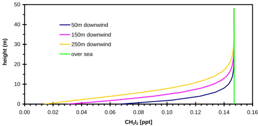
Figure 9a. Gradient of CH2I2 mixing ratios predicted using the offshore flux scenario.

Figure 9b. Gradient of CH2I2 mixing ratios predicted using the coastal flux scenario. 0 10 20 30 40 50 0.00 0.02 0.04 0.06 0.08 0.10 0.12 0.14 0.16 CH2I2 [ppt] height (m) 50m downwind 150m downwind 250m downwind over sea 0 10 20 30 40 50 0.00 0.20 0.40 0.60 0.80 1.00 1.20 1.40 1.60 1.80 2.00 CH2I2 [ppt] height (m)

directly over tidal region 50m downwind of tidal region 150m downwind of tidal region 250m downwind of tidal region

Fig. 9a. Gradient of CH2I2mixing ratios predicted using the offshore flux scenario.

Figure 9a. Gradient of CH2I2 mixing ratios predicted using the offshore flux scenario.

Figure 9b. Gradient of CH2I2 mixing ratios predicted using the coastal flux scenario. 0 10 20 30 40 50 0.00 0.02 0.04 0.06 0.08 0.10 0.12 0.14 0.16 CH2I2 [ppt] height (m) 50m downwind 150m downwind 250m downwind over sea 0 10 20 30 40 50 0.00 0.20 0.40 0.60 0.80 1.00 1.20 1.40 1.60 1.80 2.00 CH2I2 [ppt] height (m)

directly over tidal region 50m downwind of tidal region 150m downwind of tidal region 250m downwind of tidal region

Fig. 9b. Gradient of CH2I2mixing ratios predicted using the coastal flux scenario.

et al., 2000). Assuming the density is evenly spread be-tween L. digitata, L. saccharina and A. nodosum and over the intertidal zone leads to a total CH2I2 emission rate of ∼ 1.5 × 109_{molecules cm}−2_s−1_{. This rate was used as the}

maximum coastal flux at the lowest tide. The high tide flux was assumed to be equal to the offshore flux, described be-low.

Figure 5 shows that the overall magnitude of the CH2I2

concentrations predicted by the model was in good agree-ment with the observed levels, indicating that estimation of the CH2I2 flux from seaweed emissions was a valid

ap-proach. However, there were clear discrepancies in some of the features. Also shown in Fig. 5 is the modelled intertidal flux used in this scenario. At night, the flux is closely cor-related with the CH2I2concentration, with small differences

due to the variability in wind speed and eddy diffusivity. Dur-ing the day, the modelled CH2I2 concentration is reduced

relative to the tidal flux because of photolysis. However, the reduction due to photolysis was not sufficient to

simu-late the observations, as is clearly seen during the last day of data. There are also other features not well represented by the model, such as the overestimation of [CH2I2] during the

night of the 18–19 September.

3.3 Simulation of offshore emissions

An alternative flux situation was investigated, wherein the offshore region was a source of CH2I2. The atmospheric

concentration of CH2I2 predicted by the 2-dimensional

model is related to the product of the magnitude of the flux and the length of the grid. It is therefore not possible to put a meaningful value on the magnitude of the offshore flux with-out knowing precisely the length of the upwind fetch. Al-though this was known to a reasonable degree for the tidal scenario (i.e. the intertidal range), the degree of open ocean production of CH2I2is uncertain.

Ocean production of CH2I2up to 5 km offshore of Mace

Head was assessed from discrete surface seawater

(9)

16 L. J. Carpenter et al.: Coastal zone production of IO precursors L. J. Carpenter et al., Coastal zone production of IO precursors 10

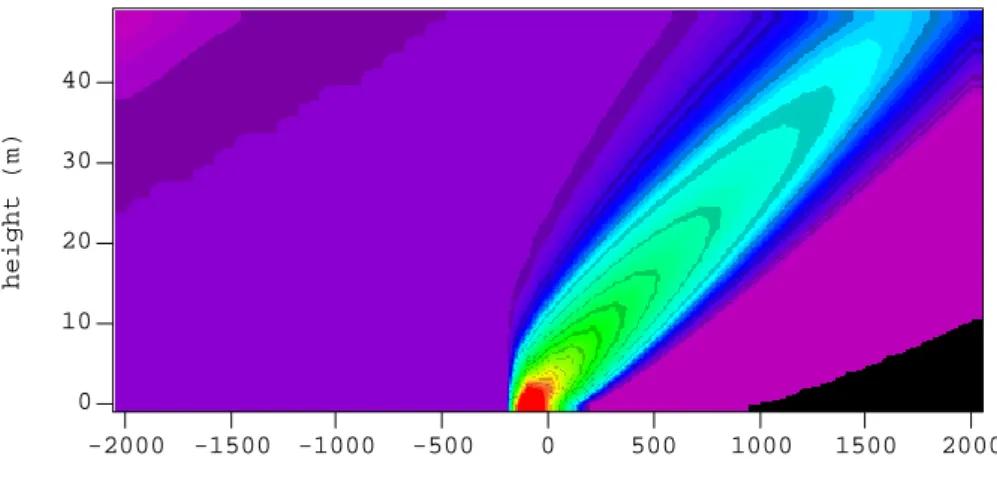
Figure 10. Predicted variation in CH2I2 concentration gradients upwind (negative distances) and

downwind (positive distances) of Mace Head at midnight. The colour scale represents the CH2I2

concentration in molecule cm-3, with black representing concentrations less than 1 x 105 molecule cm-3. -2000 -1500 -1000 -500 0 500 1000 1500 2000 40 30 20 10 0

distance from Mace Head (m)

height (m)

5.0e+006 1.7e+007 2.8e+007

Fig. 10. Predicted variation in CH2I2 concentration gradients upwind (negative distances) and downwind (positive distances) of Mace

Head at midnight. The colour scale represents the CH2I2concentration in molecule cm−3, with black representing concentrations less than 1 × 105molecule cm−3.

ments made during the 2 weeks immediately after the atmo-spheric measurements. Although there was a higher concen-tration of CH2I2in seawater sampled directly over kelp beds

then in areas with no seaweeds, there was no obvious rela-tionship between distance from shore and dissolved CH2I2

concentration between 200 m and 5 km offshore. The aver-age concentration over this region was 0.52 ± 0.26 pmol L−1 (mean of 6 measurements) and the mean seawater temper-ature was 12◦C (Carpenter et al., 2000). The equilibrium air concentration at this temperature calculated using the Henry’s law coefficient for CH2I2 reported by Moore et

al. (1995) is 0.1 pptv. Thus, it is difficult to assess whether or not the offshore waters of Mace Head were a source of

CH2I2or simply in equilibrium. An upper limit to the flux

can however be calculated using a CH2I2concentration in air

of zero. From the Liss-Merlivat expression (Liss and Merli-vat, 1986) with a square root molecular weight correction for the transfer velocity (Liss and Slater, 1974) and the mean wind speed, the flux is 2 × 105molecules cm−2s−1.

Because the offshore emissions and fetch are highly uncer-tain, we do not attempt here to provide an estimate of these emissions, but rather to provide an emission regime that re-sults in good agreement with the measurements. Thus, the point of including an offshore scenario is to establish whether non-local sources of CH2I2were present at Mace Head, and

the possible contribution of these.

With a 5 km fetch of offshore emissions, a flux of 4 ×

107molecules cm−2s−1 was required for good agreement of the overall levels of measured and modelled [CH2I2], as

shown in Fig. 6. Because a fetch of at least up to 5 km off-shore was established by the seawater measurements, this flux can be taken as an upper limit. Note, however, that the same agreement would have been possible with the es-timated flux of 2 × 105_{molecules cm}−2_s−1 _{and a fetch of}

about 1000 km. The model predictions shown in Fig. 6 were made assuming constant wind speed and eddy diffusivity (av-erages for the period). The model reproduced the daytime reductions in [CH2I2] due to photolysis, indicating that

non-local sources were indeed an important contribution to the atmospheric levels at Mace Head. However, the peak levels of CH2I2were not replicated well by the model. The

simu-lation was repeated using 40-minute averages of wind speed and eddy diffusivity. Figure 7 shows that the inclusion of micrometeorological variability resulted in significantly im-proved agreement with the measurements. Clearly, meteoro-logical parameters also played a large part in controlling the variability in CH2I2concentrations at Mace Head.

The result of including both coastal and offshore fluxes in the model is shown in Fig. 8. Although the combination of fluxes resulted in an overestimation of modelled CH2I2

con-centrations by ∼ 30%, the correlation between modelled and measured data was greater than that of either the separate flux scenarios. For ten-point averages of modelled vs mea-sured data, the r2values were 0.89 (coastal + offshore), 0.78 (offshore only) and 0.75 (coastal only).

(10)

L. J. Carpenter et al.: Coastal zone production of IO precursors 17

3.4 Prediction of spatial variation of CH2I2concentrations

The horizontal domain of the model was extended by 2 km in order to examine the dispersion of CH2I2downwind from

the shore. Both the coastal and offshore flux scenarios gave rise to similar levels of CH2I2at Mace Head at 12 m height.

However, the vertical profiles predicted were very different, as shown in Figs. 9a and 9b. The offshore source resulted in a constant CH2I2concentration vertical gradient over the open

sea, but a rapidly increasing concentration with height over Mace Head, 150 m downwind of the shore. Conversely, over a few metres height, the tidal source gave rise to decreasing

CH2I2levels over Mace Head, 50 m downwind of the tidal

region (i.e. the mid point of the 100 m cell adjacent to the 100 m tidal region). Internal boundary layer formation would lead to perturbations of these modelled gradients.

Figure 10 shows the predicted CH2I2concentrations from

2 km upwind of the site to 2 km downwind at midnight in westerly (marine) air. Considerable heterogeneity is ex-pected over the few hundred metres downwind. Measure-ments in both the horizontal and vertical domains at Mace Head are planned to test these predictions.

4 Summary and conclusions

Strong evidence for the organoiodines CH2I2 and CH2IBr

as photolytic precursors to the IO radical at Mace Head was shown from the dependence of the atmospheric concentra-tions of all three species on tidal height. Iodine oxide con-centrations peaked at low water during midday hours and the reactive organoiodines, whose atmospheric lifetimes are less than 1 hour at midday, peaked when low water coincided with night.

The intertidal flux of CH2I2upwind of Mace Head was

es-timated from seaweed emissions and used in a 2-dimensional model to predict the CH2I2concentrations in marine air at

Mace Head. This flux resulted in good agreement between the mean concentrations of measured and modelled CH2I2,

but did not reproduce well the daytime depletion due to pho-tolysis. A non-local, offshore, source of CH2I2was invoked,

which did reproduce the daytime depletion. Three separate scenarios of offshore sources alone, tidal sources alone, and offshore plus tidal sources were used as inputs to the model. The model showed that variability in wind speed and friction velocity, proximity to source, and photolysis all played im-portant roles in determining the CH2I2concentrations at the

site. The best agreement with the CH2I2 observations was

obtained using constrained micrometeorological fields, and a combination of a constant offshore flux and a tidal flux that peaked at 1.4 × 109_{molecules cm}−2_s−1_{at low water.}

Because the atmospheric concentration of CH2I2

pre-dicted by the 2-dimensional model was related to the length of the upwind fetch, a meaningful value cannot be assigned to the offshore emission rate, although we estimate an upper

limit of 4 × 107_{molecules cm}−2_s−1_{. Rather, we conclude}

that a contribution from both intertidal and offshore sources is likely, with the tidal flux being several orders of magnitude higher. Although this study cannot predict whether CH2I2

is emitted from the open ocean, it suggests that it does un-dergo air-sea exchange in coastal waters despite its presum-ably rapid photolysis rate.

Acknowledgements. We are grateful to Gerrit de Leeuw for

sup-plying micro-meteorological data from PARFORCE, and to Jochen Stutz and Gerd H¨onninger for their help performing the DOAS mea-surements and the evaluation of the DOAS data. We would also like to acknowledge Colin O’Dowd, Gerry Spain and Mick Geever for their organization of the PARFORCE campaign. Financial support for this project was provided by the Natural Environment Research Council (NERC) grant GR9/03597.

References

Alicke B., Hebestreit, K., Stutz, J., and Platt, U.: Iodine oxide in the marine boundary layer, Nature, 397, 572–573, 1999.

Allan B. J., McFiggans, G., Plane, J. M. C., and Coe, H.: Observa-tions of iodine monoxide in the remote marine boundary layer, J. Geophys. Res., 105, 14 363–14 369, 2000.

Barrie, L. A., Bottenheim, J. W., Schnell, R. C., Crutzen P. J., and Rasmussen, R. A.: Ozone destruction and photochemical reac-tions at polar sunrise in the lower Arctic atmosphere, Nature, 334, 138–141, 1988.

Barrie, L.A. and Platt, U.: Arctic tropospheric chemistry: an overview, Tellus, 49B, 450–454, 1997.

Bottenheim, J. W., Barrie, L. A., Atlas, E., Heidt, L. E., Niki, H., Rasmussen, R. A., and Shepson, P. B.: Depletion of lower tro-pospheric ozone during Arctic spring: The Polar Sunrise Exper-iment, J. Geophys. Res., 95, 18 555–18 568, 1990.

Brauers, T., Hausmann, M., Brandenburger, U., and Dorn, H.-P.: Improvement of Differential Optical Absorption Spectroscopy with a multichannel scanning technique, Applied Optics, 34, 4472–4479, 1995.

Carpenter, L. J. and Liss, P. S.: On temperate sources of bromoform and other reactive organic bromine gases, J. Geophys. Res., 105, 20, 539–548, 2000.

Carpenter, L. J., Sturges, W. T., Liss, P. S., Penkett, S. A., Alicke B., Hebestreit, K., and Platt, U.: Short lived alkyl-iodides and bro-mides at Mace Head: Links to macroalgal emission and halogen oxide formation, J. Geophys. Res, 104, 1679, 1999.

Carpenter, L. J., Malin, G., Kuepper, F., and Liss, P. S.: Novel biogenic iodine-containing trihalomethanes and other short-lived halocarbons in the coastal East Atlantic, Global Biogeochem. Cycles, 14, 1191–1204, 2000.

Cox, R. A., Bloss, W. J., Jones, R. L., and Rowley, D. M.: OIO and the Atmospheric Cycle of Iodine, Geophysical Research Letters, 26, 13, 1857–1860, 1999.

De Leeuw, G., Kunz, G. J., and O’Dowd, C. D.: Micro-meteorological measurements at the Mace Head mid-latitude coastal station, Submitted to J. Geophys. Res., 2001.

Friess, U., Wagner, T., Pundt, I., Pfeilsticker, K., and Platt, U.: Spectroscopic Measurements of Tropospheric Iodine Oxide at Neumayer Station, Antarctica, Geophys. Res. Lett., 28, 10, 1941–1944, 2001.

(11)

Gschwend, P. M., Macfarlane J. K., and Newman, K. A.: Volatile halogenated organic-compounds released to seawater from tem-perate marine macroalgae, Science, 227, 1033–1035, 1985. Harder, J. W., Brault, J. W., Johnston, P. V., and Mount, G. H.:

Temperature dependent NO2cross sections at high spectral

res-olution, J. Geophys. Res., 102, 3861–3879, 1997.

HITRAN,: HITRAN database 1986 edition, Applied Optics, 26, 4058–4097, 1987.

Hönninger, G.: Referenzspektren reaktiver Halogenverbindungen für DOAS Messungen, Diploma thesis, Ruprecht Karls Univer-sität Heidelberg, Heidelberg, 1999.

Hough, A. M.: The calculation of photolysis rates for use in global troposheric modelling studies, AERE Report R-13259, 53, HMSO, London, 1988.

Klick, S. and Abrahamsson, K.: Biogenic volatile iodated hydro-carbons in the ocean, J. Geophys. Res., 97, 12 683–12 687, 1992. Kunz, G. J., Cohen, L. H., and de Leeuw, G.: Lidar and microme-teorological measurements during the PARFORCE experiments at the Mace Head Atmospheric Research Station, Carna, Ireland, during September and June 1998, TNO Physics and Electronics Laboratory, Report FEL-00-C103, 2000.

Liss, P. S. and Merlivat, L.: Air-sea exchange rates: Introduction and synthesis, in: Role of Air-Sea Exchange in Geochemical Cycling, (Ed) Buat-M´enard, P., D. Reidel Publishing Company, Dordrecht, 113–127, 1986.

Liss, P. S. and Slater, P. G.: Flux of gases across the air-sea interface, Nature, 247, 181–184, 1974.

McFiggans, G., Allan, B., Coe, H., Plane, J. M. C., Carpenter, L. J., and O’Dowd, C., Observations of IO and a modelling study of iodine chemistry in the marine boundary layer, J. Geophys. Res., 105, 14, 371–385, 2000.

Michanek, G.: Seaweed resources of the ocean, FAO Fish. Tech. Pap., 138, 127, 1975.

Moore, R. M., Geen, C. E., and Tait, V. K.: Determination of

Henry’s Law constants for a suite of naturally occurring halo-genated methanes in seawater, Chemosphere, 30, 1183–1191, 1995.

M¨ossinger, J., Shallcross, D. E., and Cox, R. A.: UV-visible absorp-tion cross-secabsorp-tions and atmospheric lifetimes of CH2Br2, CH2I2,

and CH2BrI, J. Chem. Soc. Far., 10, 1391–1396, 1998.

Nightingale P. D., Malin, G., and Liss, P. S.: Production of chlo-roform and other low-molecular-weight halocarbons by some species of macroalgae, Limnol. Oceanogr., 40, 680–689, 1995. Peders´en, M., Coll´en, J., Abrahamsson, K., and Ekdahl, A.:

Produc-tion of halocarbons from seaweeds–an oxidative stress reacProduc-tion, Scientia Marina, 60, 257–263, 1996.

Platt, U.: Differential optical absorption spectroscopy (DOAS), Chemical Analysis Series, 127, 1994.

Platt, U. and Perner, D.: Measurements of atmospheric trace gases by long path differential UV/visible absorption spectroscopy, in: Optical and Laser Remote Sensing, (Eds) Killinger, D. A. and Mooradien, A., Springer Verlag, New York, 95–105, 1983. Schall, C., Heumann, K. G., and Kirst, G. O.: Biogenic volatile

organoiodine and organobromine hydrocarbons in the Atlantic Ocean from 42 degrees N to 72 degrees S, Fresenius J. Anal. Chem., 359, 298–305, 1997.

Stull, R. B.: An introduction to boundary layer meteorology, Kluwer Academic Publishers, Dordrecht, 1988.

Stutz, J. and Platt, U.: Improving long-path differential optical ab-sorption spectroscopy with a quartz-fiber mode mixer, Applied Optics, 36, 1105–1115, 1997.

Stutz, J., Hebestreit, K., Alicke, B., and Platt, U.: Chemistry of halogen oxides in the troposphere: comparison of model calcu-lations with recent field data, J. Atmos. Chem., 34, 65–85, 1999. Vogt, R., Sander, R., von Glasow, R., and Crutzen, P. J.: Iodine chemistry and its role in halogen activation and ozone loss in the marine boundary layer: A model study, J. Atmos. Chem., 32, 375–395, 1999.